
Intelligent Cyber Attack Detection and Classification for Network-Based Intrusion Detection Systems


Research Group on Intelligent Engineering and Computing for Advanced Innovation and Development (GECAD), Porto School of Engineering (ISEP), 4200-072 Porto, Portugal
*
Authors to whom correspondence should be addressed.
Appl. Sci. 2021, 11(4), 1674; https://0-doi-org.brum.beds.ac.uk/10.3390/app11041674
Submission received: 23 November 2020
/
Revised: 5 February 2021
/
Accepted: 8 February 2021
/
Published: 13 February 2021
(This article belongs to the Special Issue Machine Learning for Cybersecurity Threats, Challenges, and Opportunities)
Abstract
:With the latest advances in information and communication technologies, greater amounts of sensitive user and corporate information are shared continuously across the network, making it susceptible to an attack that can compromise data confidentiality, integrity, and availability. Intrusion Detection Systems (IDS) are important security mechanisms that can perform the timely detection of malicious events through the inspection of network traffic or host-based logs. Many machine learning techniques have proven to be successful at conducting anomaly detection throughout the years, but only a few considered the sequential nature of data. This work proposes a sequential approach and evaluates the performance of a Random Forest (RF), a Multi-Layer Perceptron (MLP), and a Long-Short Term Memory (LSTM) on the CIDDS-001 dataset. The resulting performance measures of this particular approach are compared with the ones obtained from a more traditional one, which only considers individual flow information, in order to determine which methodology best suits the concerned scenario. The experimental outcomes suggest that anomaly detection can be better addressed from a sequential perspective. The LSTM is a highly reliable model for acquiring sequential patterns in network traffic data, achieving an accuracy of 99.94% and an f1-score of 91.66%.
1. Introduction
At present, information and communication technology plays a vital role in the life of modern organizations. Its development has opened a wide range of new communication methods that allow faster and cheaper ways to access and share information. Modern companies increasingly rely on these technologies to provide greater availability for their clients and for managing their businesses. This dependency on information systems causes a substantial amount of sensitive user and corporate information to be shared across the network, making it more susceptible to cyber attacks that can compromise data confidentiality, integrity and availability.
An Intrusion Detection System (IDS) dynamically monitors the actions of a specific environment, for example, the network traffic, syslog records or system calls of a given operating system, in order to determine if those actions are a legitimate use or a symptom related to a given attack [1]. These systems are usually classified into Network-based Intrusion Detection Systems (NIDS) and Host-based Intrusion Detection Systems (HIDS). An NIDS works on feature vectors that comprise summarized information related to network traffic within a specified time interval while a HIDS is located on a specific host and monitors information related to the system [2].
Intrusion detection can be performed in several ways, and they usually are described as Anomaly-based Intrusion Detection or Signature-based Intrusion Detection. The latter, also known as misuse detection, attempts to detect and classify attacks by matching predefined patterns. Although maintaining reasonable levels of false alarm rates, this technique is only suitable for well-known attacks [3]. To overcome this disadvantage, some researchers have developed flexible signature-based NIDS [4,5]. On the other hand, anomaly detection aims to elaborate heuristic rules or statistical models based on the analysis of normal and abnormal activities that can further be used to classify some behaviour as benign or malicious. These systems can detect novel attacks and be combined with artificial intelligence methods to increase their detection performance.
Advances in hardware, software, and network topologies, such as the Internet of Things (IoT), mean that cyber attacks are becoming more complex and sophisticated and, therefore, more difficult to detect [6]. This dynamic nature of cyber attacks makes anomaly detection an exciting area in which to employ artificial intelligence algorithms like Neural Networks or more traditional classifiers, like Random Forests (RF), k-Nearest Neighbors (kNN) or Support Vector Machines (SVM). However, significant and realistic data from emulated network environments are required to test and compare different anomaly detection approaches and methods. The absence of reliable datasets has been identified in the literature as one of the main obstacles to intrusion detection research [7]. Nevertheless, in the last few years, some intrusion detection datasets have been published, namely CIDDS-001 [8,9], CICIDS2017 [10] and UNSW-NB15 [11]. For a detailed comparison between several NIDS datasets, the reader can consult [12].
In our research, anomaly detection for the CIDDS-001 dataset was addressed from two distinct viewpoints. The first, single-flow, consider only individual flow features. In contrast, the second, multi-flow, perform a more in-depth analysis of flow sequences, gathering more context from previous flows to detect anomalous behaviour. For each viewpoint, three state-of-the-art artificial intelligence models were employed, RF, MLP, and LSTM. By analysing these methods’ results through multiple evaluation metrics, it is possible to better understand which approach best suits the dataset and which model achieves the best performance. The objective of these techniques is not only to detect malicious behaviour but also to specify the nature of that behaviour by identifying the respective attack type through a multi-class classification process. A model trained for binary classification with Normal and Attack labels would not be able to recognise which type of attack was performed, only that an anomalous situation it had occurred on the network.
This work was developed within the Security of Air Transport Infrastructures of Europe (SATIE) project, as research for a novel approach to investigate the temporal correlation between cyber and physical alerts. The SATIE project will build a holistic, interoperable, and modular security toolkit to be exploited by the next generation of Airport Operation Centres and Security Operation Centres to protect critical air transport infrastructures against combined cyber–physical threats [13].
Our work introduces several novelties, and mainly differs from others presented in Section 2 because, to the best of our knowledge:
- No work has addressed the target variable AttackType of the CIDDS-001 in order to perform multi-class classification for intrusion detection;
- Only Gwon et al. in [14] has addressed network intrusion detection from a sequential perspective by using LSTM. However, the experimental results were achieved for the UNSWNB-15 dataset, which is two years older than the CIDDS-001, contains considerably less data for training and testing, and regards different attack types to those presented in the CIDDS-001 dataset;
- Only in [15], was LSTM used for the CIDDS-001 dataset. Nevertheless, the work does not mention any study about the flow window size and its impact in the model’s evaluation metrics. It is also important to highlight that, in [15], only the External Server data was used and the Class label was selected as target value. This analysis is different to the one presented in our work;
- No previous work has established a proper comparison between the two intrusion detection approaches addressed in our work: single-flow and multi-flow;
- Our work was performed in the context of the SATIE project and the methods described in this research will become part of it’s modular security toolkit to be used by the next generation of Security Operation Centres to protect critical air transport infrastructures.
The paper is organized in multiple sections that can be detailed as follows. Section 2 provides a comparison between the current research and previous works on the CIDDS-001 dataset as well as a description of other implementations of the same methods for other relevant datasets. Section 3 briefly explains the machine learning models that were used, the problem’s viewpoints and the considered evaluation metrics. In Section 4, the obtained results are presented and discussed. Section 5 provides a summary of the main conclusions that can be drawn from this research and appoints further research topics that can be addressed.
2. Related Work
In the last few years, several works have tested different machine and deep learning models on the CIDDS-001 dataset. These experiments addressed the target variable Class and, in general, attempted to classify each flow as either Suspicious, Unknown, Normal, Attacker or Victim. This particular work, although being related to previous research, considers a different target variable and, therefore, performs a substantially different analysis of the dataset. The AttackType attribute was used as label in order to train the selected models to not only identify the occurrence of a given attack but also detect the type of attack that has been performed. Nevertheless, it is very important to understand what conclusions have been drawn from prior and related work on the CIDDS-001 dataset.
In [16], Tama et al. evaluated the performance of a Deep Neural Network (DNN) for conducting anomaly detection in an IoT environment. To assure a reliable performance analysis, several validation methods, such as cross-validation and repeated cross-validation, were performed on different datasets, namely, CIDDS-001, UNSW-NB15 and GPRS [17]. A grid-search was conducted in order to find the appropriate hyper-parameters of the DNN for each dataset. The model achieved nearly 100% accuracy for the the CIDDS-001 dataset (using Class as target variable).
In [18], Verma and Ranga performed an analysis of the CIDDS-001 dataset from the machine learning point of view. Both k-NN Classifier and k-Means Clustering methods performed well. A comparative analysis between CIDDS-001 and other existing benchmarking datasets is appointed as a future research topic in order to measure the complexity of this dataset compared to others.
In [15], Althubiti et al. used the CIDDS-001 External Server data to test a Long-Short Term Memory (LSTM) model. The data were split into for training and for testing. The LSTM achieved a greater performance when compared with other methods, namely SVM, Naïve Bayes (NB) and Multi-Layer Perceptron (MLP). Although sequence size is not mentioned, most of the hyperparameter values that were used are described in detail. Nicholas et al., in [19], also evaluated the performance of an LSTM model in the flow-based data of CIDDS-001 and compared the obtained results with other traditional classifiers.
In [20], Abdulhammed et al. addressed the problem of disproportional class distribution. The research considered only the flows which corresponded to the target values Normal and Attack for the dataset’s Class label and employed several class-balancing techniques, such as minority class up-sampling, majority class down-sampling, spread sub-sampling and class balancing by assigned weights inversely proportional to class frequencies. The authors, although believing that the results may not be generalized to a broader range of problems, concluded that class unbalance had a slight impact on the classification process for that specific situation. Advantages of the usage of RF for anomaly detection have been appointed, such as the ability to estimate missing data and maintain reasonable accuracy values even when a large proportion of data is missing.
Finally, in [2], Rashid et al. performed a comparative analysis between the benchmark datasets NSL-KDD and CIDDS-001. A hybrid feature selection method was used in order to reduce the number of attributes of each dataset and six machine learning models were tested. For the CIDDS-001 dataset, NB and k-NN achieved the best results with an accuracy score of . A detailed comparison between deep learning methods, such as Convolutional Neural Networks (CNN), Deep Belief Networks (DNB) and Recurrent Neural Networks (RNN) have been appointed as further research. The authors also mentioned the possibility of applying feature learning on the raw data of network traffic headers in order to stimulate the maximum potential of neural networks.
None of the works mentioned above addressed multi-class classification to detect distinct attack types for the CIDDS-001 dataset. Only the Class label was used for distinguishing between Normal, Attacker, Victim, Suspicious and Unknown classes. No work has used the AttackType target variable for identifying and categorizing attack attempts. Additionally, only in [15] was the LSTM used for the context of CIDDS-001, and the work does not mention any study regarding flow window sizes and its impact on the methods performance. Some other works that have also studied LSTMs for network-based intrusion detection systems in the context of other well-established datasets such as UNSW-NB15 and CICIDS2017 can be described as follows.
In [21], Roy and Cheung, presented, within the IoT environment, a novel technique for anomaly detection using a Bi-directional LSTM network. The model was trained and tested in a smaller randomly selected sample of the UNSW-NB15 dataset and obtained substantially good results, namely an accuracy score of and a f1-score value of . Similarly to [15], sequence size was not mentioned.
In [14], Gwon et al. used an LSTM model with a feature-embedding layer on the UNSW-NB15 dataset, obtaining excellent results. Instead of using traditional encoding methods for the categorical variables, the authors employed a word embedding layer that transformed those variables into numeric vectors that were able to translate their inherited semantic meaning. Network-based anomaly detection was addressed from a sequential perspective, and flaws of traditional classifiers were appointed, since they struggle to learn sequential patterns from data. The LSTM model was selected to overcome this problem since it can analyse entire sequences of flows and learn meaningful patterns from sequential data. Learning strategies such as many-to-one or many-to-many were carefully studied, and the performance of the model was analysed for different sequence sizes. For binary classification, the model achieved an accuracy score of , while for multi-class, the accuracy score was .
In [3], He et al., proposed a combination of a Multimodal Deep Auto Encoder (MDAE) and an LSTM for conducting anomaly detection. This novel approach was tested on three datasets from 1999 to 2017, namely, NSL-KDD, UNSW-NB15 and CICIDS2017 achieving, for multi-class classification, accuracy scores of 80.20%, 86.20% and 98.60%, respectively.
It is important to state that in [14], LSTMs were used to address intrusion detection from a sequential perspective, combining patterns from both individual flows and sequences of flows. However, the experimental results were obtained in the context of the UNSWNB-15 dataset, which is older than CIDDS-001, resembles a smaller data collection and contains several attack types, such as Shellcode, Backdoors and Worms, which are considerably distinct from the ones presented in CIDDS-001.
Our work presents a novel analysis on the CIDDS-001 by using the AttackType label to perform a multi-class classification process and highlights the benefits of using machine learning for processing a stream of network flows to accurately detect and categorize malicious behaviour on network traffic. Two deep learning methods, LSTM and MLP, and one machine learning method, RF, were selected to be employed based on the results presented in the literature. RF was chosen over other well-known methods since it obtained the best overall results in the the broader scope of intrusion detection research. For example, in [22], the performance of several machine learning models were analysed in the context of the KDD99 dataset and RF achieved an accuracy score of , greater than the accuracy of other techniques such as SVMs, Naive Bayes and Logistic Regression. Similarly, in [23], several methods were tested on four distinct datasets, including CIDDS-001, and RF presented the best average accuracy value over all datasets, , in comparison to other models such as AdaBoost and Extreme Gradient Boosting.
3. Materials and Methods
This section describes the main characteristics and properties of the selected dataset as well as the nature of the machine and deep learning techniques that were applied. Each model is briefly explained and all configurations and parameters are detailed. The employed evaluation metrics are also carefully explained so that the comparison between methods can be better understood. The objectives of our study can be described as follows:
- Compare single-flow and multi-flow approaches for attack detection in the context of network-based intrusion detection systems;
- Understand the effect of temporal dependencies in intelligent attack detection and classification;
- Understand how the performance of an ML algorithm is affected by the size of the flow window;
- Use the AttackType label of the CIDDS-001 as target variable in order to perform multi-class classification for intrusion detection.
3.1. Dataset Description
The Coburg Intrusion Detection Data Set (CIDDS-001), disclosed by Markus Ring et al. in [8], contains about four weeks of network traffic from 5:43:57 p.m., 3 March 2017 up until 11:59:30 p.m., 18 April 2017, comprising a total of nearly 33 million flows captured from two different environments, an emulated small business environment (OpenStack) and an External Server that captured real and up-to-date traffic from the internet. The OpenStack environment includes several clients and typical servers like an E-Mail server or a Web server. The dataset contains labeled flow-based data that can be used to evaluate anomaly-based network intrusion detection systems considering normal activity as well as DoS, Brute Force, Ping Scans and Port Scan attacks. The python scripts used for traffic generation can be found in a github repository [24].
The CIDDS-001 is a very reliable dataset for studying and evaluating network-based intrusion detection methods since it is considerably recent, comprises a considerable collection of network flows and regards several up-to-date attack types. The collection of data provided by the CIDDS-001 dataset is represented in a unidirectional Netflow format. Table 1 provides an overview of the dataset attributes. All attributes from 1 to 12 are default Netflow features, whereas those from 13 to 16 result from the labelling process.
Regarding the AttackType label, CIDDS-001 is a very unbalanced and realistic dataset. The majority class corresponds to benign traffic. Each of the other classes represents one of four distinct attack types that are not equally distributed over time. Table 2 describes the attack type distribution over time.
For the OpenStack environment, only the first two weeks contain data related to attacks while the remaining weeks only contain benign behaviour. On the other hand, for the External Server, the first week does not contain any attack attempt and the remaing three weeks onyl contain instances of the DoS and Port Scan attack types.
3.2. Data Preprocessing and Sampling
In order to train the Machine Learning methods, the CIDDS-001 data first had to be preprocessed. The data were first analysed in order to detect errors, duplicated values and inconsistent data. Some abnormalities were found, such as the Flows column, with the same value for each dataset entry and the Bytes columns representation for its numerical values being 1K instead of 1000. Thereby, the Flows column was removed as well as three other columns that correspond to labels not considered in our study, Class, AttackID and AttackDescription. Only AttackType was considered because this research is focused on the evaluation of different machine- and deep-learning approaches for attack recognition and specification. Some additional transformations were also done to correct the Bytes column, such as replacing “K” for and “M” for and then converting the corresponding result to its correct numeric representation. The Date first seen feature was used to index the data in order to preserve the flow sequence.
After these operations seven categorical features and three numerical features remained. The resulting feature vector is composed of the following features: Src IP, Src Port, Dest IP, Dest Port, Proto, Flags, ToS, Duration, Bytes and Packets. Since the input value of the employed algorithms is expected to be a numerical matrix, all non-numerical features, such as Src IP and Dst IP, were encoded into a representative numerical form using the ordinal encoding method. Finally, every feature was normalized between 0 and 1 using min–max normalization to enhance the performance of the mentioned techniques. Min–max scales look at each feature individually according to the following equation
where represents the scaled value of x.
As previously stated, the dataset comprises a total of nearly 33 million flows. Due to this considerable number of flows, high hardware requirements are needed to conduct this study. In order to solve this problem and substantially decrease the required amount of memory, processing power and time, only a portion of the data were used.
Since one of the objectives of this research is to better understand the effect of temporal dependencies in intelligent attack detection and classification, a random and stratified split approach could not be used because it would not preserve the flow sequence. Hence, efforts were made to find a smaller flow interval that could be used a good representation of the dataset, with instances of every attack and similar class proportions. Thereby, only the first two weeks of OpenStack environment were considered since they contain instances of every attack type, and a sample of 2,535,456 flows between 2:18:05 p.m., 17 March 2017 and 5:42:17 p.m., 20 March 2017 was selected. Table 3 establishes a comparison in terms of size and class proportion between the chosen sample, the first two weeks of OpenStack environment and the whole dataset.
3.3. Models
One machine learning model, Random Forest [20], and two deep learning models, Multi-Layer Perceptron [25] and Long-Short Term Memory [14,15] were employed. These state-of-the-art techniques for intrusion detection systems presented very promising results in previous research for multiple state-of-the-art datasets, namely for the CICIDS2017 [10] and the UNSW-NB15 [11]. In order to better understand the main differences in each technique, a brief description of their nature is provided as well as all the considered parameters and configurations.
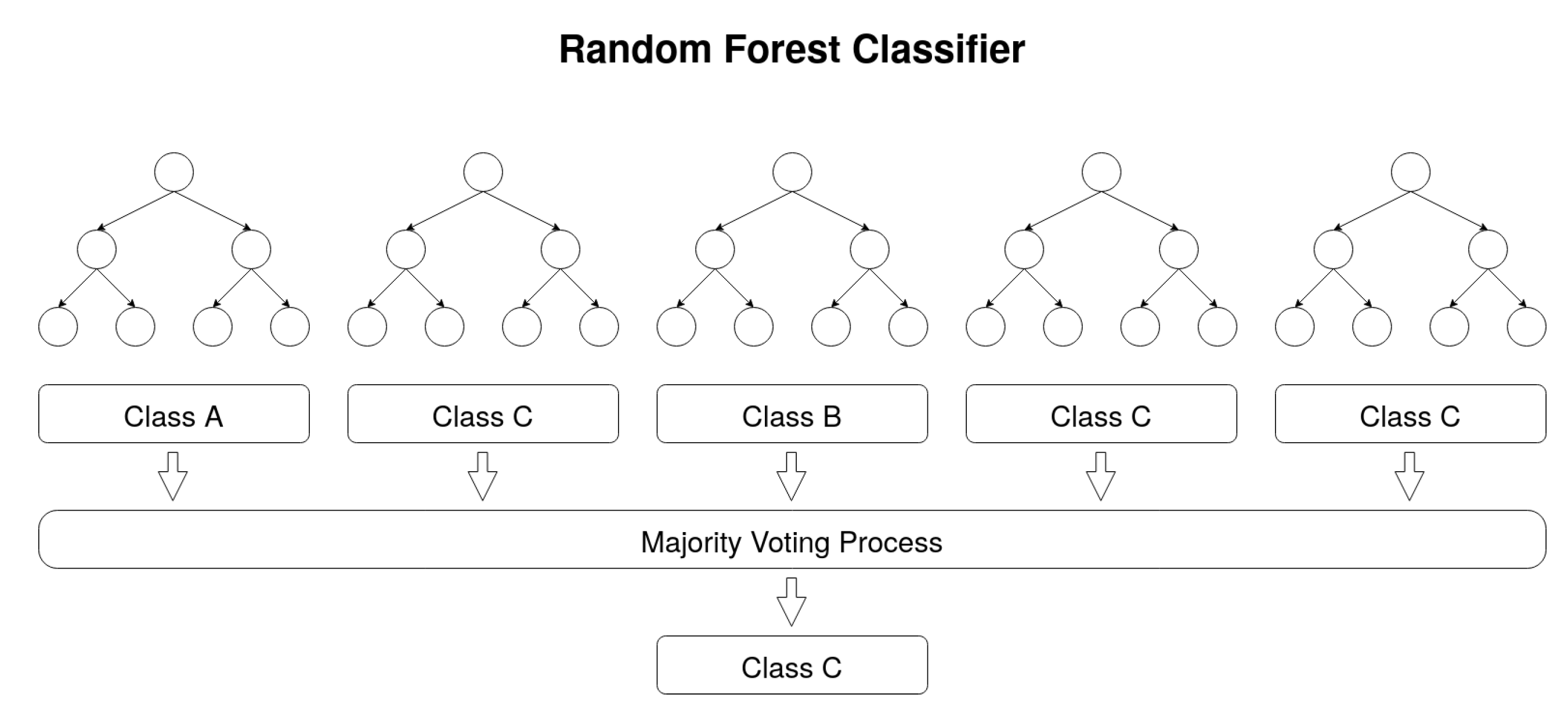
Random Forest Classifier [26]. A Random Forest (RF) consists in a large number of Decision Trees that operate together as an ensemble. Each Decision Tree is a decision tool that works in a tree-like model of decisions and outcomes. For a given dataset entry, each tree of a Random Forest model predicts a given class and the most voted one is elected as the model’s output. The underlying theory behind Random Forests is the wisdom of crowds. In order to assure good performance, the algorithm must be trained with good representative data and the correlation between the predictions of each tree must be low [27]. Figure 1 represents the behaviour of the classifier.
The Random Forest Classifier has multiple parameters that can be configured. Table 4 summarizes some important parameters that were applied.
Max tree depth was set to 35 to prevent the occurrence of overfitting and to ensure generalization. Class weights were adjusted to be inversely proportional to class frequencies in the input data in order to avoid poor classification on the minority classes, since the CIDDS-001 dataset is highly unbalanced [20]. This way, it was possible to tune the classifier to favor the minority classes over the majority classes by using weights obtained through the following equation
where is the weight of class one, is the number of occurrences of class one in the input data and represents the total number of samples of the input.
The remaining values for the number of estimators, split criterion, min samples split, min samples leaf and max features were set to the default of Scikit-learn [28] python library, since they are recognised as well established configurations for a vast majority of contexts.
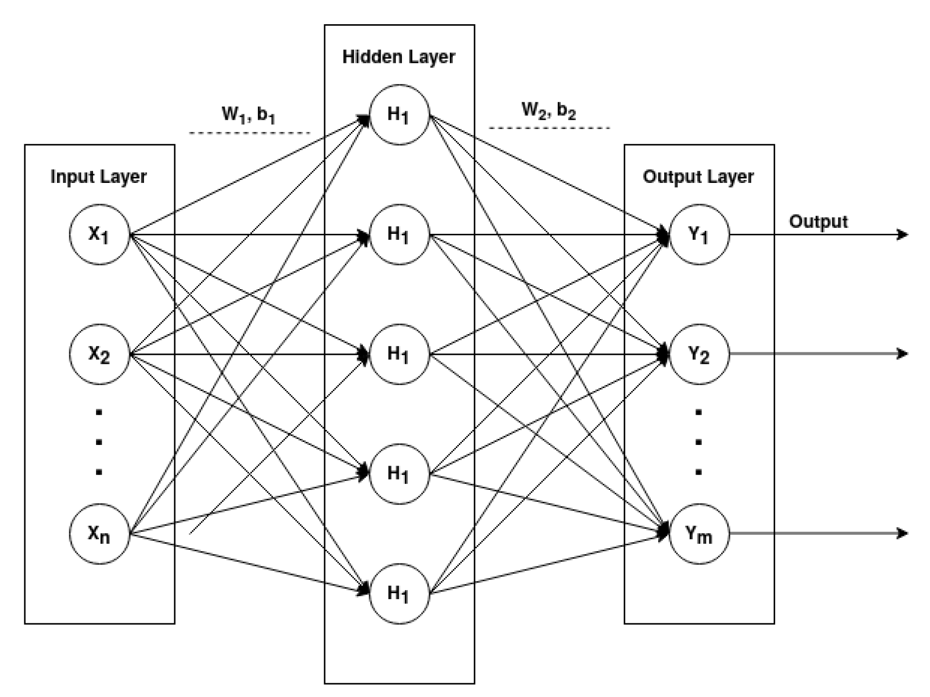
Multi-Layer Perceptron [29]. A Multi-Layer Perceptron (MLP) is a type of Feed-Forward Network which can be represented as an acyclic graph with no feedback connections (the outputs of the model are not fed back into itself). An MLP comprises three or more layers, having one input layer, one or more hidden layers and an output layer, in which each layer has multiple neurons that can be represented in mathematical notation.
Each hidden layer can be mathematically described by
where is the input vector, is the weights vector, is the bias and f is a non-linear activation function like sigmoid, hyperbolic tangent or softmax (preferred for the output layer). These activation function are mathematically represented as
where x defines a given input.
Figure 2 graphically represents a fully connected architecture of a MLP with one input layer, one hidden layer and one output layer.
The employed MLP consists of the four-layered architecture described in Table 5. The input layer node number is the same as the number of considered features, 10 for single flow classification and 10 multiplied by the window size for multi-flow. The output layer node is 5, the same as the number of different categories for the AttackType label. Two hidden layers of 100 neurons each were considered. For each layer, a Dropout probability of 0.2 was used. This method will remove some of the next layer inputs (20%) in order to reduce the probability of overfitting.
Rectified Linear Unit (ReLU) was selected as the activation function of the hidden layers. This activation function has proven to be very computationally efficient and it was one of the main breakthroughs in the neural network history for reducing the vanishing and exploding gradient phenomenon [30]. Its mathematical representation is
where x defines the input.
Softmax was used for the output layer since it assigns decimal probabilities to the prediction of each class in a multi-classification problem. The sum of all probabilities adds up to one. Categorical Cross-Entropy was chosen as loss objective function and Adam was used as optimization function. The batch size was set to 1024, the epoch size to 50 and an early stopping method was employed in order to stop the training as soon as the loss value stabilized. The learning rate was set to 0.001 to avoid a quick convergence to a sub-optimal solution.
Table 6 summarizes the main configurations of the MLP model.
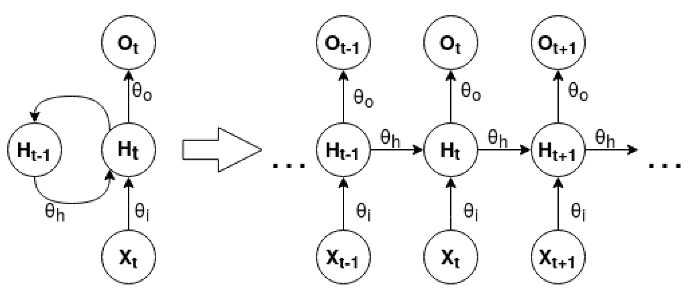
Long-Short Term Memory [31,32]. A Long-Short Term Memory (LSTM) is a type of Recurrent Neural Network (RNN). An RNN contains feedback connections that allow information to travel in a loop from layer to layer. These networks store information about past computations through a hidden state that represents the network memory. Therefore, the output, , for a given input, , at a given timestep, t, is influenced by the inputs of its previous timesteps, , where n defines the total number of prior timesteps. This characteristic allows RNNs to be very suited to working with sequential data. Figure 3 represents the unfold form of a standard many to many RNN.
Unfold is a concept associated with RNN graphical representation. The network is expanded according to the size of its input and output sequence. RNN can be modeled for one to one, one to many, many to one and many to many problems. The difference between each of the presented problems is the distinct cardinality between the input and output of the network. An RNN can be mathematically expressed by the following equations [33]
where is the input, is the output and is the hidden state at a given timestep t. is the hidden state of previous timestep and comprises the weights and biases of the network.
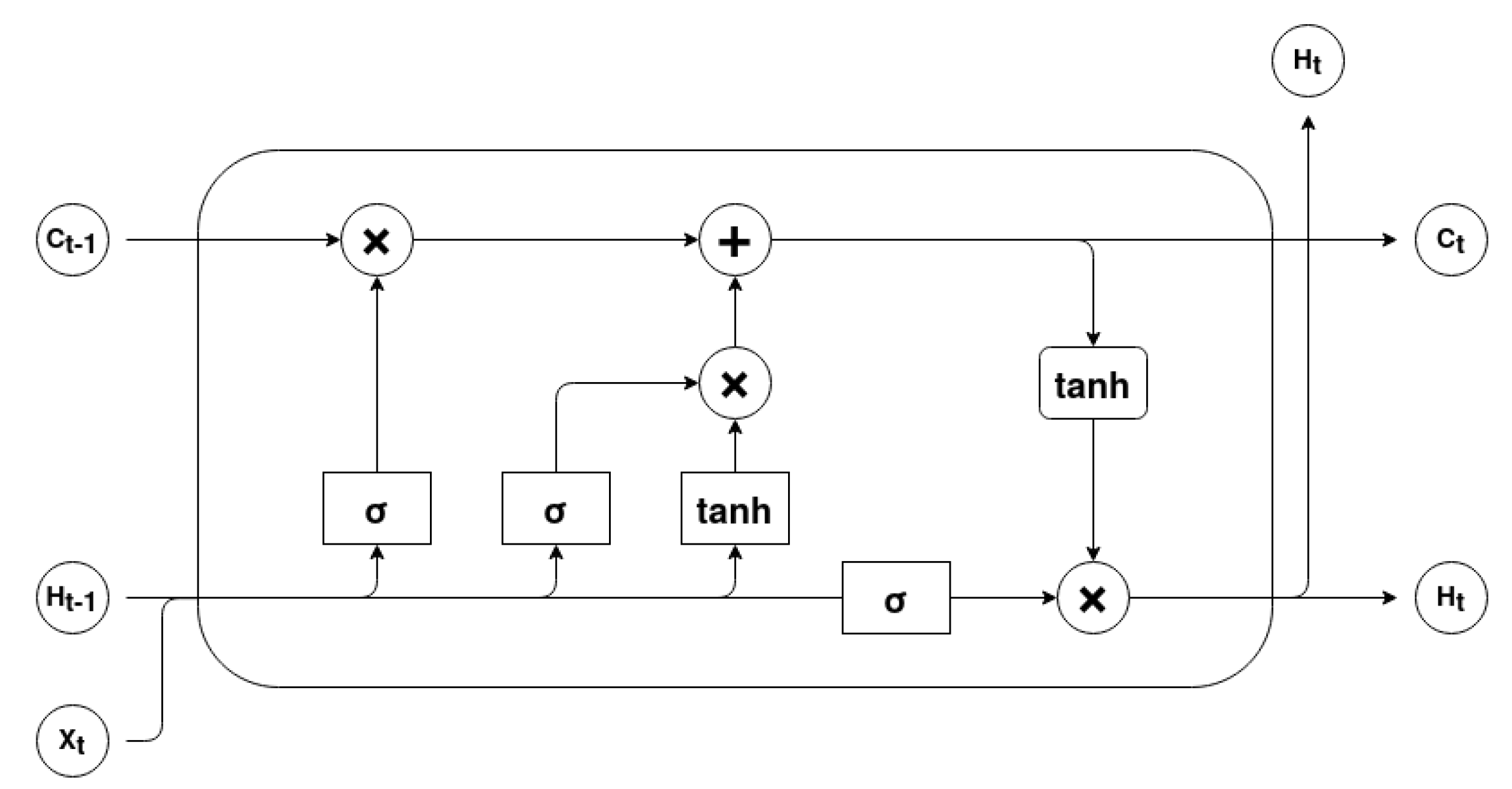
RNNs’ main issue is that they have difficulties in learning long-term relationships between the elements of the input sequence due to the vanishing and exploding gradient problem. LSTM cells were designed to overcome this problem through the use of cell memory and gating units. Therefore, an input at a given timestep t can change or even override the cell state. This process is carefully regulated by three gating units, the input gate, the forget gate and the output gate [34]. Figure 4 describes the basic architecture of an LSTM cell.
The forget gate is a sigmoid layer that outputs a result between 0 and 1 for each value of the cell state . This results determines which information should be erased or kept. It can be mathematically represented as
The input gate determines which values should be updated and the tanh layer creates a vector of candidate values . The current cell state, , results from the addition of the forget computation, obtained by the multiplication of and , with the scaled candidate values. This process can be represented by the following equations
The output gate establishes the output information. The sigmoid layer determines what cell status information will be output. The cell state is processed by hyperbolic tangent in order to scale its values between −1 and 1. Finally the multiplication between these outputs is the LSTM cell output value. The process can be mathematically defined as
The employed LSTM network model has one input layer of shape (1, 10), two hidden layers with 100 nodes each, and one output layer with five nodes, one for each class. Changes in the length of the flow window implies alterations in the input shape from (1, 10) to (Window Size, 10). Each hidden layer has Dropout set to 0.2 to prevent the network to overfit the training data. Table 7 describes the employed LSTM network architecture.
The LSTM network configurations are the same as the ones configured for the MLP. Categorical Cross-Entropy remains as the loss objective function and an Adam optimizer with a default 0.001 learning rate was used. The number of epochs was set to 50 and batch size to 1024. Table 8 summarizes the main configurations of the LSTM model.
3.4. Anomaly Detection
In our research, anomaly detection is addressed from two distinct viewpoints. The first viewpoint consists of finding patterns in single-flow features, while the second attempts to make a more informed analysis by considering an entire sequence of flows. For the single-flow viewpoint, each enumerated technique was trained with the preprocessed data of the CIDDS-001 dataset. RF and MLP expected a 2D matrix as input, while LSTM, which was specifically designed for sequential data, requires a 3D input. Figure 5 exemplifies how the two dimensional CIDDS-001 preprocessed data and its corresponding 3D transformation can be visualized.
The multi-flow approach addresses the problem from a different point of view. Patterns acquired from single-flow features can be insufficient to correctly detect and differentiate anomalies. From a temporal and sequential analysis of a given window of flows, it is possible to combine individual patterns with short- to long-term relations between flows, which can potentially lead to better results. In order to conduct this analysis, data had to be reorganized and prepared to reflect the intended temporal properties. The original 2D data were reshaped to a 3D format by performing an one-to-one window overlap. For a selected window size s, a dataset entry can be defined as , where x is a given flow at a given timestep t. Algorithm 1 describes how the introduced transformation was implemented.
| Algorithm 1 Pseudo-code for the data reshape algorithm |
|
Suppose a given entry, , contains flows. In that case, the first s rows of the algorithm’s output matrix should be disregarded because they have invalid data due to the insufficient number of previous timesteps. For this study, the first 99 rows were removed to ensure that the algorithms are trained and tested with the same data, regardless of the selected window size (which is never higher than this value).
As previously explained, LSTM is a model designed to deal with three-dimensional data and already expects a 3D matrix as input, while RF and MLP require the conventional 2D input. To provide such an input, the sequential data were flattened into a two-dimensional space. This operation implies no distinction between the features of independent flows and that data, although containing information from previous timesteps, cannot be interpreted as a sequence. This process is represented in Figure 6.
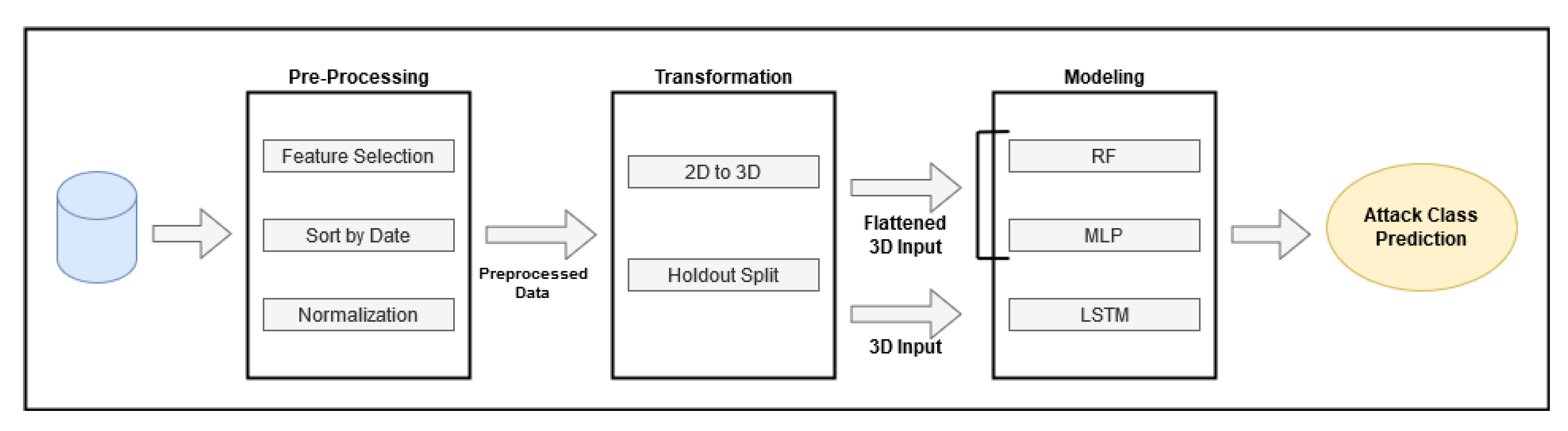
In conclusion, in our approach the network traffic data are first preprocessed, removing the least meaningful features, then the flows are ordered in chronological order and the resultant feature vector is transformed into a numerical representative form, as explained in Section 3.2 Then, the preprocessed data are transformed to a three-dimensional format according to a given window size and split into train, validation and test sets. For the RF and MLP models, the 3D data are reshaped into a corresponding 2D format, and for the LSTM, the data are directly used in their 3D representation. Finally, each model produces predictions, which are evaluated by the metrics described in Section 3.5.
Regarding the hold-out method, 70% of the total data were selected for training, while the remaining 30% were used for testing. From the training set, 10% of data were set aside for validation. The full scope of our approach is summarized in Figure 7.
3.5. Evaluation Metrics
Several metrics, such as Accuracy, Recall, Precision and F1-Score, can be used to evaluate the performance of a given classifier [35]. However, these metrics’ employment should not be made carelessly, particularly in intrusion detection systems, where high-class imbalance situations are relatively common. This section will briefly describe the metrics used in this research, their mathematical representation [36], and how they can be interpreted to better understand the results obtained from applying the previously enumerated methods.
Accuracy is one of the most common metrics used in classification problems and usually gives a reliable measure of the model’s performance. It can be calculated through the following equation [28]
where is the number of samples of a given dataset, is the vector of predicted values, is the corresponding vector of true values and I is the indicator function, which returns 1 if matches and 0 otherwise.
In this particular case, due to the fact that CIDDS-001 is a very unbalanced dataset, accuracy is not a good metric to use. In the selected sample, 82.53% of the flows are benign traffic. Even if the classifier fails to classify every other attack class and only predicts the benign flows correctly, it would still achieve an accuracy value of 82.53%. When working with unbalanced data, the accuracy is biased towards the majority class. To overcome this situation, other metrics were considered.
In terms of the number of true positives (TP), false positives (FP), false negatives (FN), and true negatives (TN) reported by the confusion matrix, the macro-averaged precision can be expressed as follows
Precision measures the number of labels a model has incorrectly predicted to be positive that were actually negative. is the number of flows correctly classified as class and is the amount of flows whose true value corresponds to a given class , where that were incorrectly labeled as .
On the other hand, recall expresses the ability of a model to find relevant instances in a dataset. Macro-averaged recall can be defined as
where stands for the number of flows of a class that were incorrecly labeled as a class .
F1-score is a metric that considers both precision and recall through the computation of their harmonic mean. The macro-averaged f1-score is well suited for unbalanced datasets such as CIDDS-001, and it can be mathematically described as
False Positive Rate (FPR), or Fall-Out, expresses the probability of false alarm and can be determined by the following mathematical statement
In this research, results are expressed through all the above measures. Understanding each evaluation metric and each employed model’s nature is crucial to making sense of the obtained results.
4. Results and Discussion
The results presented and discussed in this section derive from the implementation of the previously described models, viewpoints, and metrics through the usage of the Python programming language and its appropriate libraries.
- Scikit-learn [28] was used to implement RF and to preprocess data;
- Matplotlib [41] was used for result visualization.
The required hardware support was granted by Google Colab [42], which provided free access to virtual machines equipped with GPUs and significant disk space and RAM. Since the resources on Colab are not guaranteed and not unlimited, the amount of available RAM and GPU type can vary over time. Therefore, it was impossible to perform a reliable comparison between the computing time costs of the employed methods.
4.1. Single-Flow
For the single-flow viewpoint, each model was trained and tested with the the CIDDS-001 preprocessed data. Table 9 summarizes the obtained results.
Even though there are few differences between each model’s accuracy results, the values for the other metrics are quite different. LSTM presents the highest precision score with little recall, while RF presents the highest recall value with considerably less precision. On the other hand, MLP exhibits a minor difference between its precision and recall values. This balance translates into a better f1-score value than the one related to the LSTM model. The f1-score for the RF model is substantially greater than the ones presented by every other technique. Regarding the FPR, the RF assures fewer occurrences of false alarms than both the LSTM and MLP.
The combination of high accuracy values and differentiated f1-scores can lead to the conclusion that models performed quite differently on the minority classes. Figure 8 expresses the f1-score values of each model for every class.
The RF performed better for the Ping Scan class than every other model. Since the Ping Scan class only represents 0.04% of the total sample data, this class’s misclassification has little effect on the accuracy value. For the macro-averaged f1-score, this does not happen, because the misclassification of any class, more or less prevalent in the sample, translates into a heavy penalization in its value.
From the general perspective, choosing the best model for this experiment is not a straightforward process. The RF assures that most of the attacks are detected even with the occurrence of a considerable amount of false-positive errors, while the LSTM fails to detect a significant quantity of attacks but grants a lower occurrence of such errors. Regarding the balance between precision and recall, RF outperforms the remaining techniques, but that is only significant when compliant with the deployment situation’s requirements and constraints.
4.2. Multi-Flow
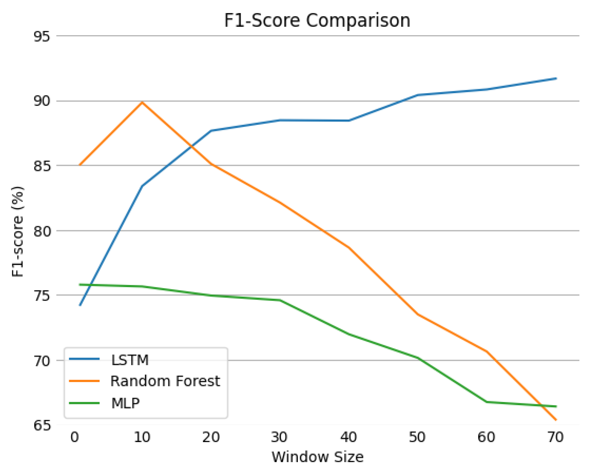
From the multi-flow viewpoint, the CIDDS-001 preprocessed data were transformed as multiple sequences, and several window sizes from 0 to 70 were used. Figure 9 describes the evolution of the f1-score for each model as the window size increases.
The LSTM’s f1-score increases alongside the window size while the corresponding score for the remaining models consistently decreases. Despite this trend, the RF model for a window of 10 flows presented an f1-score of . This result is considerably close to the best recorded value, , exhibited by the LSTM for the maximum window size.
A possible explanation for the decrease in the f1-score value for the RF model after reaching such a relevant result and the consistent increase in the values presented by the LSTM can be related to the nature of these techniques. While the LSTM model has a cell state carefully regulated by gates that allow it to learn only meaningful short-term relationships across a given sequence of flows (independently of its size), the RF model was not designed to deal with sequential data. With the increase in window size, the feature space of each entry for the RF substantially increases as well. Its inability to learn sequence-based relationships from data can potentially lead to worse results with the increase in feature space. On the other hand, Random Forests generally behave quite well with noise and are not prone to suffering from overfitting. Table 10 compares the scores of the RF and LSTM models that exhibited the best f1-score results.
Both techniques presented significant results, with LSTM exhibiting better recall scores and slightly less precision. Although RF’s performance worsens as the window size increases, it is still a quite reliable model for recognising patterns in small sequences of flows. The LSTM model scores are more consistent and could potentially be even better for larger window sizes. The value of FPR is the same for both approaches.
Since f1-score is obtained through the harmonic mean of precision and recall, analysis of these metrics can be important to better understand each model’s behaviour. Figure 10 translates the variations in the RF’s and LSTM’s precision and recall values.
Regarding the RF, for the 10 flow window, the precision value increased from to while the recall decreased from to . These results contributed to the better f1-score result of the RF, . As the window size increased, both precision and recall values became smaller, resulting in consistently lower f1-scores until reaching the value of for a window size of 70. On the other hand, in the LSTM, for a window of 10 flows, precision dropped from to and recall increased from to . This trade-off resulted in a better balance between the values of each metric, which translated into a greater f1-score value. Although casual decreases have occurred for some sequence lengths, both precision and recall were consistently better for further window sizes.
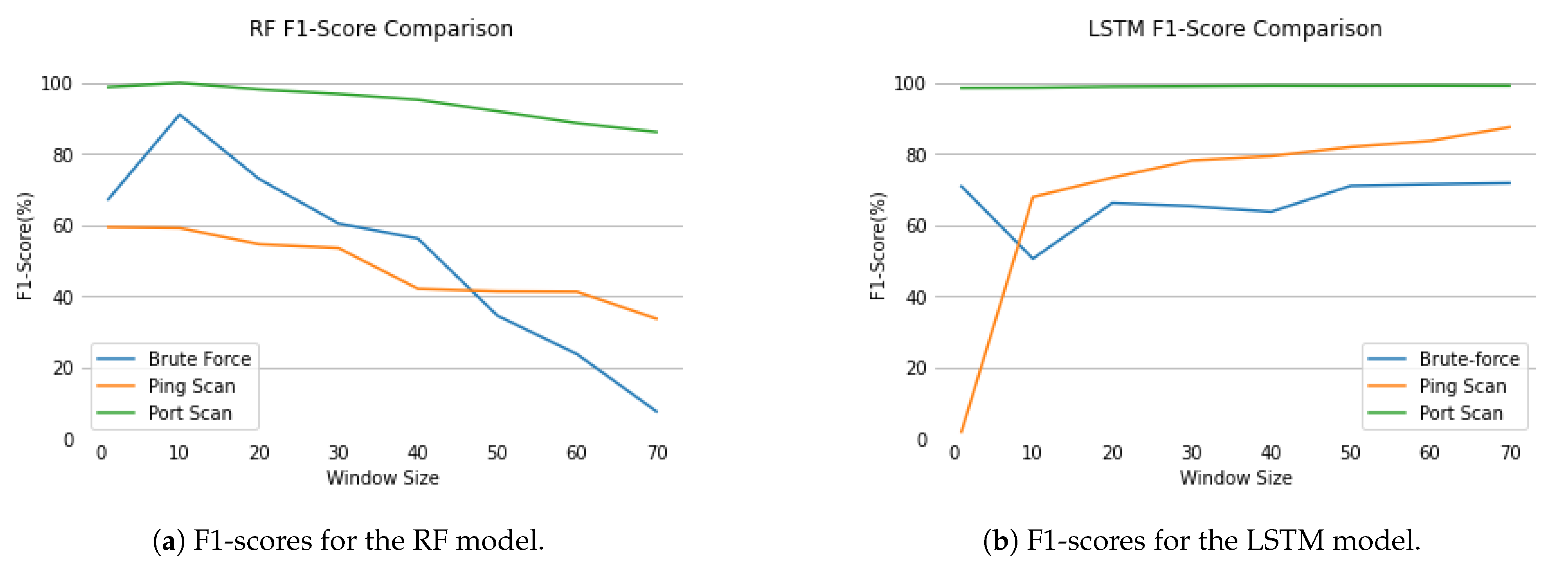
Macro-averaged f1-score can also be detailed by understanding how the individual score for each class evolved. Figure 11 expresses the RF and LSTM model’s behaviour for the minority classes.
The most prevalent classes were not represented because there were no significant changes in their values. For the RF, at window size 10, the f1-score for the Brute Force class reaches its peak at , explaining the increase in the overall f1-score of the model. For larger window sizes, the f1-score of all classes, Brute Force, Ping Scan and Port Scan, rapidly decreased. Concerning the LSTM, for the DoS class, the score remained at 99.99, for attack absence at 99.77, and for Port Scan it increased from 98.48 to 99.12. Regarding the minority classes, despite the considerable drop in Brute Force’s f1-score for the 10 flow window, it steadily increased from 70.84 to 71.76 for further sizes. On the other hand, the Ping Scan class presented the most relevant increase, from to .
The presented results can lead to the interpretation that the LSTM is able to detect consistently more attacks with less false-positive errors as the flow sequences grow larger. This general improvement does not seem to imply favoring one class performance over another, as the f1-score of every class either remained the same or increased.
To ensure that the model has been trained properly, the learning curves, represented in Figure 12, were carefully studied.
The loss value decreases over each epoch for both training and validation sets without any evidence of the occurrence of underffiting or overffiting. The accuracy score for both sets is also quite similar and it slowly improves as loss value is minimized.
4.3. Conclusions
Overall, it can be concluded that anomaly-based intrusion detection for the CIDDS-001 dataset can be better addressed from a multi-flow perspective. The obtained results lead to the interpretation that an analysis that considers features from individual flows, as well as patterns expressed by flow sequences with specific lengths, builds a considerably better classification model. The LSTM model’s employment has proven to be very promising for detecting such patterns in data compared with other state-of-the-art techniques. Its performance as a classifier seems to get better as the flow sequence size increases.
5. Conclusions
Our work addressed the CIDDS-001 dataset using the AttackType label to train machine-learning methods, such as RF, MLP, and LSTM, to correctly classify a given network flow as either benign or as a DoS, Brute Force, Ping Scan, or Port Scan attack. The employed models were implemented from two distinct perspectives, single-flow and multi-flow, and the obtained results were compared in order to determine which was best-suited to the concerned scenario.
For the single-flow perspective, only individual flow characteristics were addressed by the models, and RF achieved the best result, with an f1-score of . On the other hand, for the multi-flow viewpoint, both individual flow features and short- to long-term relationships between flows of a given sequence were considered. Several sequence sizes were tested and the best f1-score value, , was obtained by the LSTM model for a window size of 70. Although the performance of the RF considerably drops with the increase in sequence length, for a window size of 10, it achieved a f1-score of , which is relatively close to the best recorded value. From the results, it can be concluded that learning sequential relationships between flows seem to improve anomaly detection considerably. The LSTM has proven to be a very reliable model for capturing these sequential patterns, and its performance appears to get better for bigger flow sequences.
This research was very important to conclude that, within the SATIE project’s scope, LSTM is an interesting approach to deal with the temporal complexity of security alerts with multiple heterogeneous sources. This technique will be part of a Machine Learning module to be integrated into an investigation tool, where security operators can better grasp the context of incident occurrence.
In the future, it would be pertinent to train the LSTM for larger windows in order to better understand the model’s behaviour. More refined feature engineering and data preparation methods can be performed to improve the results, and other LSTM architectures with attention mechanisms can further be experimented with. Meta-heuristic methods such as Genetic Algorithms could also be employed to maximize the optimization of the algorithm’s hyper-parameters.
Author Contributions
Conceptualization, I.P., N.O. and E.M.; methodology, I.P. and N.O.; implementation, N.O.; validation, I.P. and O.S.; investigation, E.M. and N.O.; writing, I.P., N.O. and O.S.; supervision, I.P. and O.S.; project administration, I.P.; funding acquisition, I.P. All authors have read and agreed to the published version of the manuscript.
Funding
This project has received funding from the European Union’s Horizon 2020 research and innovation programme under grant agreement number 832969.
Institutional Review Board Statement
Not applicable.
Informed Consent Statement
Not applicable.
Data Availability Statement
Publicly available datasets were analyzed in this study. This data can be found here: CIDDS-001.
Conflicts of Interest
The authors declare no conflict of interest. The funders had no role in the design of the study; in the collection, analyses, or interpretation of data; in the writing of the manuscript, or in the decision to publish the results.
References
- Debar, H.; Dacier, M.; Wespi, A. Towards a taxonomy of intrusion-detection systems. Comput. Netw. 1999, 31, 805–822. [Google Scholar] [CrossRef]
- Rashid, A.; Siddique, M.J.; Ahmed, S.M. Machine and Deep Learning Based Comparative Analysis Using Hybrid Approaches for Intrusion Detection System. In Proceedings of the 2020 3rd International Conference on Advancements in Computational Sciences (ICACS), Lahore, Pakistan, 17–19 February 2020; pp. 1–9. [Google Scholar]
- He, H.; Sun, X.; He, H.; Zhao, G.; He, L.; Ren, J. A Novel Multimodal-Sequential Approach Based on Multi-View Features for Network Intrusion Detection. IEEE Access 2019, 7, 183207–183221. [Google Scholar] [CrossRef]
- Papamartzivanos, D.; Gómez Mármol, F.; Kambourakis, G. Introducing Deep Learning Self-Adaptive Misuse Network Intrusion Detection Systems. IEEE Access 2019, 7, 13546–13560. [Google Scholar] [CrossRef]
- Hu, Z.; Li, Z.; Wu, J. A Novel Network Intrusion Detection System (NIDS) Based on Signatures Search of Data Mining. In Proceedings of the First International Workshop on Knowledge Discovery and Data Mining (WKDD 2008), Adelaide, SA, Australia, 23–24 January 2008; pp. 10–16. [Google Scholar]
- Vinayakumar, R.; Alazab, M.; Soman, K.P.; Poornachandran, P.; Al-Nemrat, A.; Venkatraman, S. Deep Learning Approach for Intelligent Intrusion Detection System. IEEE Access 2019, 7, 41525–41550. [Google Scholar] [CrossRef]
- Małowidzki, M.; Berezinski, P.; Mazur, M. Network Intrusion Detection: Half a Kingdom for a Good Dataset. In Proceedings of the NATO STO SAS-139 Workshop; 2015; Available online: https://pdfs.semanticscholar.org/b39e/0f1568d8668d00e4a8bfe1494b5a32a17e17.pdf (accessed on 2 February 2021).
- Ring, M.; Wunderlich, S.; Gruedl, D.; Landes, D.; Hotho, A. Flow-based benchmark data sets for intrusion detection. In Proceedings of the 16th European Conference on Cyber Warfare and Security (ECCWS); ACPI: Dublin, Ireland, 2017; pp. 361–369. [Google Scholar]
- Ring, M.; Wunderlich, S.; Scheuring, D.; Landes, D.; Hotho, A. Creation of Flow-Based Data Sets for Intrusion Detection. J. Inf. Warf. 2017, 4, 40–53. [Google Scholar]
- Sharafaldin, I.; Habibi Lashkari, A.; Ghorbani, A. Toward Generating a New Intrusion Detection Dataset and Intrusion Traffic Characterization. In ICISSP; University of New Brunswick (UNB): Fredericton, NB, Canada, 2018; pp. 108–116. [Google Scholar]
- Moustafa, N.; Slay, J. UNSW-NB15: A comprehensive data set for network intrusion detection systems (UNSW-NB15 network data set). In Proceedings of the 2015 Military Communications and Information Systems Conference (MilCIS), Canberra, ACT, Australia, 10–12 November 2015; pp. 1–6. [Google Scholar]
- Ring, M.; Wunderlich, S.; Scheuring, D.; Landes, D.; Hotho, A. A survey of network-based intrusion detection data sets. Comput. Secur. 2019, 86, 147–167. [Google Scholar] [CrossRef] [Green Version]
- SATIE-Security of Air Transport Infrastructure of Europe. 2020. Available online: http://satie-h2020.eu/ (accessed on 2 September 2020).
- Gwon, H.; Lee, C.; Keum, R.; Choi, H. Network Intrusion Detection based on LSTM and Feature Embedding. arXiv 2019, arXiv:1911.11552. [Google Scholar]
- Althubiti, S.A.; Jones, E.M.; Roy, K. LSTM for Anomaly-Based Network Intrusion Detection. In Proceedings of the 2018 28th International Telecommunication Networks and Applications Conference (ITNAC), Sydney, NSW, Australia, 21–23 November 2018; pp. 1–3. [Google Scholar]
- Adhi Tama, B.; Rhee, K.H. Attack Classification Analysis of IoT Network via Deep Learning Approach. Res. Briefs Inform. Commun. Technol. Evolut. 2017, 3, 1–9. [Google Scholar]
- Vilela, D.W.F.L.; Ferreira, E.W.T.; Shinoda, A.A.; de Souza Araújo, N.V.; de Oliveira, R.; Nascimento, V.E. A dataset for evaluating intrusion detection systems in IEEE 802.11 wireless networks. In Proceedings of the 2014 IEEE Colombian Conference on Communications and Computing (COLCOM), Bogota, Colombia, 4–6 June 2014; pp. 1–5. [Google Scholar]
- Verma, A.; Ranga, V. Statistical analysis of CIDDS-001 dataset for Network Intrusion Detection Systems using Distance-based Machine Learning. Procedia Comput. Sci. 2018, 125, 709–716. [Google Scholar] [CrossRef]
- Nicholas, L.; Ooi, S.Y.; Pang, Y.; Hwang, S.; Tan, S.Y. Study of long short-term memory in flow-based network intrusion detection system. J. Intell. Fuzzy Syst. 2018, 35, 5947–5957. [Google Scholar] [CrossRef]
- Abdulhammed, R.; Faezipour, M.; Abuzneid, A.; AbuMallouh, A. Deep and Machine Learning Approaches for Anomaly-Based Intrusion Detection of Imbalanced Network Traffic. IEEE Sens. Lett. 2019, 3, 1–4. [Google Scholar] [CrossRef]
- Roy, B.; Cheung, H. A Deep Learning Approach for Intrusion Detection in Internet of Things using Bi-Directional Long Short-Term Memory Recurrent Neural Network. In Proceedings of the 2018 28th International Telecommunication Networks and Applications Conference (ITNAC), Sydney, NSW, Australia, 21–23 November 2018; pp. 1–6. [Google Scholar]
- Saranya, T.; Sridevi, S.; Deisy, C.; Chung, T.D.; Khan, M. Performance Analysis of Machine Learning Algorithms in Intrusion Detection System: A Review. Procedia Comput. Sci. 2020, 171, 1251–1260. [Google Scholar] [CrossRef]
- Verma, A.; Ranga, V. Machine Learning Based Intrusion Detection Systems for IoT Applications. Wirel. Pers. Commun. 2020, 111, 2287–2310. [Google Scholar] [CrossRef]
- Ring, M.; Wunderlich, S.; Gruedl, D.; Landes, D.; Hotho, A. Generation Scripts for the Coburg Intrusion Detection Data Sets (Cidds). 2017. Available online: https://github.com/markusring/CIDDS (accessed on 11 May 2020).
- Zhiqiang, L.; Mohi-Ud-Din, G.; Bing, L.; Jianchao, L.; Ye, Z.; Zhijun, L. Modeling Network Intrusion Detection System Using Feed-Forward Neural Network Using UNSW-NB15 Dataset. In Proceedings of the 2019 IEEE 7th International Conference on Smart Energy Grid Engineering (SEGE), Oshawa, ON, Canada, 12–14 August 2019; pp. 299–303. [Google Scholar]
- Breiman, L. Random forests. Mach. Learn. 2001, 45, 5–32. [Google Scholar] [CrossRef] [Green Version]
- Yiu, T. Understanding Random Forest. 2019. Available online: https://towardsdatascience.com/understanding-random-forest-58381e0602d2 (accessed on 15 May 2020).
- Cournapeau, D. Scikit-learn Documentation. Available online: https://scikit-learn.org/ (accessed on 15 May 2020).
- Kain, N.K. Understanding of Multilayer Perceptron (MLP). 2018. Available online: https://medium.com/@AI_with_Kain/understanding-of-multilayer-perceptron-mlp-8f179c4a135f/ (accessed on 26 May 2020).
- Glorot, X.; Bordes, A.; Bengio, Y. Deep Sparse Rectifier Neural Networks. In Proceedings of Machine Learning Research, Proceedings of the Fourteenth International Conference on Artificial Intelligence and Statistics, Fort Lauderdale, FL, USA, 11–13 April 2011; Gordon, G., Dunson, D., Dudík, M., Eds.; PMLR: Fort Lauderdale, FL, USA, 2011; Volume 15, pp. 315–323. [Google Scholar]
- Hochreiter, S.; Schmidhuber, J. Long Short-Term Memory. Neural Comput. 1997, 9, 1735–1780. [Google Scholar] [CrossRef] [PubMed]
- Van Houdt, G.; Mosquera, C.; Nápoles, G. A Review on the Long Short-Term Memory Model. Artif. Intell. Rev. 2020, 53, 5929–5955. [Google Scholar] [CrossRef]
- McGonagle, J.; Williams, C.; Khim, J. Recurrent Neural Network. Available online: https://brilliant.org/wiki/recurrent-neural-network/ (accessed on 12 May 2020).
- Olah, C. Understanding LSTM Networks. 2015. Available online: https://colah.github.io/posts/2015-08-Understanding-LSTMs/ (accessed on 14 May 2020).
- Sokolova, M.; Lapalme, G. A systematic analysis of performance measures for classification tasks. Inf. Process. Manag. 2009, 45, 427–437. [Google Scholar] [CrossRef]
- Döring, M. Performance Measures for Multi-Class Problems. 2018. Available online: https://www.datascienceblog.net/post/machine-learning/performance-measures-multi-class-problems/ (accessed on 15 May 2020).
- Oliphant, T. NumPy Documentation. 2020. Available online: https://numpy.org/index.html (accessed on 19 May 2020).
- McKinney, W. Pandas Documentation. Available online: https://pandas.pydata.org/ (accessed on 16 May 2020).
- Abadi, M.; Barham, P.; Chen, J.; Chen, Z.; Davis, A.; Dean, J.; Devin, M.; Ghemawat, S.; Irving, G.; Isard, M.; et al. TensorFlow: A System for Large-Scale Machine Learning. In Proceedings of the 12th USENIX Symposium on Operating Systems Design and Implementation (OSDI 16), Savannah, GA, USA, 2–4 November 2016; pp. 265–283. [Google Scholar]
- Chollet, F. Keras Documentation. Available online: https://keras.io/ (accessed on 20 May 2020).
- Hunter, J.D. Matplotlib Documentation. 2020. Available online: https://matplotlib.org/ (accessed on 19 May 2020).
- Bisong, E. Google Colaboratory. In Building Machine Learning and Deep Learning Models on Google Cloud Platform: A Comprehensive Guide for Beginners; Apress: Berkeley, CA, USA, 2019; pp. 59–64. [Google Scholar]
Figure 1.
Representation of Random Forest prediction process.

Figure 2.
Architecture of a Multi-Layer Perceptron.


Figure 4.
Basic LSTM cell architecture (adapted from [34]).
Figure 4.
Basic LSTM cell architecture (adapted from [34]).

Figure 5.
Single flow input visualization. The x axis stands for the number of features of each flow, the y represents the number of samples and the z, required for the LSTM input, corresponds to the number of timesteps (1 timestep for single flow).
Figure 5.
Single flow input visualization. The x axis stands for the number of features of each flow, the y represents the number of samples and the z, required for the LSTM input, corresponds to the number of timesteps (1 timestep for single flow).

Figure 6.
Multi-flow as a two-dimensional space. The x axis stands for the number of features, y represents the number of samples and z describes the number of time steps.
Figure 6.
Multi-flow as a two-dimensional space. The x axis stands for the number of features, y represents the number of samples and z describes the number of time steps.

Figure 7.
Anomaly Detection Approach.

Figure 8.
Single-Flow f1-score values of the LSTM, RF and MLP models for the Brute Force, DoS, No Attack, Ping Scan and Port Scan classes.
Figure 8.
Single-Flow f1-score values of the LSTM, RF and MLP models for the Brute Force, DoS, No Attack, Ping Scan and Port Scan classes.

Figure 9.
Evolution of the f1-score for the LSTM, RF and MLP models as the window size increase.

Figure 10.
Precision and recall values for the RF and LSTM models as window size increases.

Figure 11.
F1-score changes for the minority classes for the RF and LSTM models.

Figure 12.
LSTM training and validation learning curves.


Table 1.
Specification of the CIDDS-001 dataset features. Adapted from [8].
Table 1.
Specification of the CIDDS-001 dataset features. Adapted from [8].
| N° | Name | Desription |
|---|---|---|
| 1 | Src IP | Source IP Address |
| 2 | Src Port | Source Port |
| 3 | Dest IP | Destination IP Address |
| 4 | Dest Port | Destination Port |
| 5 | Proto | Transport Protocol (e.g., ICMP, TCP, or UDP) |
| 6 | Date first seen | Start time flow first seen |
| 7 | Duration | Duration of the flow |
| 8 | Bytes | Number of transmitted bytes |
| 9 | Packets | Number of transmitted packets |
| 10 | Flags | OR concatenation of all TCP Flags |
| 11 | Tos | Type of Service |
| 12 | Flows | Not specified |
| 13 | Class | Class label (Normal, Attacker, Victim, Suspicious and Unknown) |
| 14 | AttackType | Type of Attack (PortScan, DoS, Bruteforce, PingScan) |
| 15 | AttackID | Unique Attack id. Allows attacks which belong to the same class carry the same attack id |
| 16 | AttackDescription | Provides additional information about the set attack parameters (e.g., the number of attempted password guesses for SSH-Brute-Force attacks) |
Table 2.
Attack distribution over time.
| Open Stack | External Server | |||||||
|---|---|---|---|---|---|---|---|---|
| Week | DoS | Brute-Force | Ping Scan | Port Scan | Dos | Brute-Force | Ping Scan | Port Scan |
| 1st | Yes | Yes | Yes | Yes | No | No | No | No |
| 2nd | Yes | Yes | Yes | Yes | Yes | No | No | Yes |
| 3rd | No | No | No | No | Yes | No | No | Yes |
| 4th | No | No | No | No | Yes | No | No | Yes |
Table 3.
AttackType class distribution comparison.
| Class | Dataset | OpenStack 1st Half | Sample |
|---|---|---|---|
| Total Records | 32,630,424(100%) | 18,762,253(100%) | 2,535,456(100%) |
| Brute Force | 9888(0.03%) | 4992(0.03%) | 1262(0.05%) |
| DoS | 2,959,027(9.07%) | 2,959,027(15.77%) | 390,440(15.40%) |
| No Attack | 29,352,063(89.95%) | 15,526,226(82.75%) | 2,092,550(82.53%) |
| Ping Scan | 6090(0.02%) | 6090(0.03%) | 1068(0.04%) |
| Port Scan | 303,356(0.93%) | 265,918(1.41%) | 50,136(1.98%) |
Table 4.
Summary of Random Forest configuration.
| Parameter | Value |
|---|---|
| N° of Estimators | 100 |
| Split Criterion | Gini Impurity |
| Max Depth | 35 |
| Min Samples Split | 2 |
| Min Samples Leaf | 1 |
| Max Features | |
| Class Weights | Balanced |
Table 5.
Employed MLP architecture.
| Layer | Size | Activation | Dropout |
|---|---|---|---|
| Dense | 10 × Window | - | - |
| Dense | 100 | ReLU | 0.2 |
| Dense | 100 | ReLU | 0.2 |
| Dense | 5 | Softmax | - |
Table 6.
Summary of MLP configuration.
| Parameter | Value |
|---|---|
| Epoch | 50 |
| Batch Size | 1024 |
| Optimizer | Adam |
| Learning Rate | 0.001 |
| Objective Loss | Categorical Cross-Entropy |
Table 7.
Employed LSTM network architecture.
| Layer | Size | Activation | Dropout |
|---|---|---|---|
| Dense | (Window, 10) | - | - |
| Dense | 100 | Tanh | 0.2 |
| Dense | 100 | Tanh | 0.2 |
| Dense | 5 | Softmax | - |
Table 8.
Summary of LSTM configuration.
| Parameter | Value |
|---|---|
| Epoch | 50 |
| Batch Size | 1024 |
| Optimizer | Adam |
| Learning Rate | 0.001 |
| Objective Loss | Categorical Cross-Entropy |
Table 9.
Single-Flow results for the LSTM, RF and MLP models.
| Single-Flow (%) | |||||
|---|---|---|---|---|---|
| Model | Accuracy | Precision | Recall | F1-Score | FPR |
| LSTM | 99.91 | 98.37 | 71.40 | 74.23 | 0.05 |
| RF | 99.90 | 79.43 | 95.68 | 85.04 | 0.02 |
| MLP | 99.92 | 78.68 | 73.75 | 75.79 | 0.06 |
Table 10.
Comparison between the f1-scores of LSTM-70 and RF-10.
| Multi-Flow (%) | |||||
|---|---|---|---|---|---|
| Model | Accuracy | Precision | Recall | F1-Score | FPR |
| LSTM-70 | 99.94 | 94.03 | 89.71 | 91.66 | 0.04 |
| RF-10 | 99.95 | 96.83 | 85.65 | 89.82 | 0.04 |
Publisher’s Note: MDPI stays neutral with regard to jurisdictional claims in published maps and institutional affiliations. |
© 2021 by the authors. Licensee MDPI, Basel, Switzerland. This article is an open access article distributed under the terms and conditions of the Creative Commons Attribution (CC BY) license (http://creativecommons.org/licenses/by/4.0/).
Share and Cite
MDPI and ACS Style
Oliveira, N.; Praça, I.; Maia, E.; Sousa, O. Intelligent Cyber Attack Detection and Classification for Network-Based Intrusion Detection Systems. Appl. Sci. 2021, 11, 1674. https://0-doi-org.brum.beds.ac.uk/10.3390/app11041674
AMA Style
Oliveira N, Praça I, Maia E, Sousa O. Intelligent Cyber Attack Detection and Classification for Network-Based Intrusion Detection Systems. Applied Sciences. 2021; 11(4):1674. https://0-doi-org.brum.beds.ac.uk/10.3390/app11041674
Chicago/Turabian StyleOliveira, Nuno, Isabel Praça, Eva Maia, and Orlando Sousa. 2021. "Intelligent Cyber Attack Detection and Classification for Network-Based Intrusion Detection Systems" Applied Sciences 11, no. 4: 1674. https://0-doi-org.brum.beds.ac.uk/10.3390/app11041674
Note that from the first issue of 2016, this journal uses article numbers instead of page numbers. See further details here.