High-Speed Elevator Car Air Pressure Compensation Method Based on Coupling Analysis of Internal and External Flow Fields

Abstract

As the demand for high-speed elevators grows, the requirements of elevator performance have also developed. The high speed will produce strong airflow disturbances and drastic pressure changes, which is prone to cause passenger discomfort. In this paper, an elevator car air pressure compensation method based on coupling analysis of internal and external flow fields (IE-FF) is proposed. It helps to adaptively track the ideal air pressure curve (IAPC) inside the car and controls the air pressure fluctuation to improve the ride comfort of the elevator. To obtain the air pressure transient value in the elevator car, an IE-FF modeling method is proposed. Based on the IE-FF model, the air pressure compensation system is developed. To realize the air pressure compensation inside the car, an adaptive iterative learning control (A-ILC) algorithm is proposed, to eliminate the passengers’ ear pressing due to the severe air pressure fluctuation. To verify the proposed method, the KLK2 (Canny Elevator Co., Ltd., 2015, Suzhou, China) high-speed elevator is applied. The numerical experiment results show that the proposed method has higher tracking accuracy and convergence speed compared to the classical Proportion Integral Differential (PID) algorithm and the Proportion Integral-iterative learning control (PD-ILC) algorithm.

1. Introduction

As the demand for a quick elevator speed rises, the high-speed (running speed between 5$\mathrm{m}/{\mathrm{s}}^2$ to 8$\mathrm{m}/{\mathrm{s}}^2$) and ultra-high-speed (running speed larger than 8$\mathrm{m}/{\mathrm{s}}^2$) elevators are becoming more and more widely used. While the increases in elevator speed can improve transportation efficiency, passenger discomfort has gradually become prominent [1]. When a high-speed elevator runs fast in the hoistway, it will produce strong airflow disturbances and drastic pressure changes due to the small cross-section of the hoistway and the complex structure of the elevator [2]. In addition, air pressure fluctuations outside the car will be directly transmitted to the car due to the existence of the ventilation system and leakage gaps. Instantaneous large air pressure changes in the car will cause passengers to have obvious ear pressing. Air pressure compensation during elevator operation can effectively reduce air pressure fluctuation amplitude and keep the elevator running smoothly and comfortably.

There are two main research methods for the aerodynamics of high-speed elevators. One is to build a test platform to conduct experiments to obtain the elevator’s aerodynamic data during operation. The other is to numerically solve the aerodynamic characteristics of the elevator through the simulation modeling. Duan et al. [3] simulated the running status of an elevator according to different design parameters under various operating conditions and measured the instantaneous velocity field of the different elevator car shrouds. Zhu et al. [4] obtained the aerodynamic characteristics of high-speed elevators and found that traction ropes and counterweights have a significant influence on airflow disturbances using an aerodynamic analysis of high-speed elevators. Bai et al. [5] carried out experiments to measure the aerodynamic characteristics of high-speed elevators. They analyzed the effects of different shapes of car and hoistway parameters on the aerodynamic characteristics of the elevator. Matsuda et al. [6,7] found that the effect of high-speed elevator cars and airflow produce strong airflow disturbances and aerodynamic noise, which are far higher than the mechanical noise. Wang et al. [8] utilized the static incompressible Navier–Stokes equations to numerically simulate the three-dimensional turbulence of a high-speed elevator hoistway. Shi et al. [9] established a two-dimensional model of unsteady turbulence of the high-speed elevator system. They focused mainly on the transient changes of aerodynamics on the car when a counterweight moves in the hoistway. Mei et al. [10] realized the dynamic simulation optimization by utilizing a proposed dynamic byte coding genetic algorithm.

At present, there are few researches on the law of air pressure changes in high-speed elevator cars. However, there has been many researches on pressure fluctuations in enclosed passenger compartments such as high-speed trains. In fact, the running state of high-speed elevators and high-speed trains has great similarities. Therefore, the research method of high-speed trains has a high reference value for the relative research of high-speed elevators. Hara [11] developed a comprehensive formula for the overall pressure rise across the compression wave front in a cylindrical tunnel based on the general equations of steady-flow gas dynamics. Vardy [12] developed an equivalent formulation, but accounted for the preexisting airflow, which could be quite important. Sockel [13,14] obtained a rather simple formula providing the amplitude of the first two pressure peaks as a function of the main parameters, such as the Mach number and the blockage ratio, and allowing for skin friction forces on the tunnel and train surfaces. Anthoine [15] presented a review of the current state of understanding of tunnel entrance aerodynamics for high-speed trains and an experimental assessment of the performance of countermeasures to reduce the slope of the initial pressure rise. Biotto et al. [16] implemented a discontinuous Galerkin (DG) method for the solution of the one-dimensional equations of variable area flow to simulate the pressure wave generated by a train travelling through a tunnel. Yoon and Lee [17] applied an approximate compact Green’s function to calculate the compression wave from a train entering a tunnel. In addition, they proposed a new method that couples the Kirchhoff formulation with the Euler equation to solve the generation and propagation of the compression wave. Through the analogy of the pipeline flow model, Klaver and Kassies [18] established a calculation model for vehicle interior pressure by using pressure and time to reflect vehicle airtightness parameters, referred to as the flow model. Schwanitz et al. [19,20] investigated the effect of pressure variation on discomfort for high-speed train passengers and acquired the continuous assessments of pressure events using sliders and retrospective assessments. Sanz-Andres and Santiago-Prowald [21] presented a simple analytical model for the train-induced flow and its effects on pedestrians. The expressions developed for the induced air velocity and pressure on the pedestrian surface, as well as their dependence with time, were obtained from the unsteady potential theory. Moreover, aiming at the horizontal wind effect on the aerodynamic performance of coaxial tri-rotor vehicle, Lei et al. [22] obtained the streamline distribution, pressure distribution, velocity contour and vortex distribution with different horizontal wind conditions throughout the numerical simulations. The change in the aerodynamic performance can be used for reference by the high-speed elevator car air pressure compensation research.

The severe air pressure fluctuation in enclosed passenger compartments is prone to cause the issue of passenger discomfort, such as ear pressing. The air pressure compensation and control is significant to improve passenger comfort. Aimed at the problem of human ear discomfort caused by air pressure changes in elevator cars, Yamamoto [23] proposed a method to reduce the lifting speed as the lifting distance becomes longer to slow down the air pressure change. Hitachi Elevator Company invented an elevator car air pressure control device [24], which used a fan to fill or extract air into the car to control the pressure in the car to change according to the set air pressure curve. Mizuno et al. [25] developed an air pressure control system to control air pressure inside elevator cars to a steady rate of change. Based on the Internet of Things (IoTs) big data, Zhang et al. [26] proposed an adaptive iterative learning control algorithm to restrain the pressure fluctuation in the train according to the quasi-periodicity and repeatability of mass data in the process of train running in tunnels. Wen et al. [27] proposed a kind of digital pressure control project to solve the problem of pressure fluctuation inside the high-speed train carriage. Li and Chen [28] established a fuzzy-PID controller to adjust the gain parameters of the Proportion Integral Differential (PID) by using the fuzzy algorithm, so as to better adjust the working frequency of the air-conditioning fan, and to restrain, in real-time, the transmission of pressure from the outside to the inside of the train.

While the existing research on the law of change, adjustment, compensation and control of the air pressure of the high-speed elevator car has been scarce, the relative research methods of the high-speed train can be as references due to the similarity of operating status. When a high-speed elevator runs quickly in a narrow and long shaft, it will cause strong airflow disturbances and drastic air pressure changes, which will have a great impact on the stability and the ride comfort of the elevator. To improve the ride comfort of a high-speed elevator, an air pressure compensation system can be applied to actively compensate and adjust the air pressure inside the elevator car, which can effectively eliminate the passengers’ ear pressing due to the severe air pressure fluctuation. In view of this, an elevator car’s air pressure compensation method based on coupling analysis of internal and external flow fields (IE-FF) has been proposed to adaptively track the ideal air pressure curve (IAPC) inside the car, so as to realize the compensation and control of the air pressure in the car. To obtain the transient air pressure in the elevator car, an IE-FF coupling variation model, based on the characteristic of the flow field inside and outside the car, is established by considering the transmission of air pressure fluctuations inside and outside the car. Based on the IE-FF coupling variation model, an air pressure compensation system is developed and an adaptive iterative learning control (A-ILC) algorithm is proposed to adjust the air pressure inside the car in real time.

The remainder of this paper is organized as follows. The IE-FF coupling model based on the characteristic of the flow field inside and outside the car is proposed and the air pressure compensation system is developed in Section “Air pressure compensation based on IE-FF coupling model”. The A-ILC algorithm is proposed in Section “Air pressure compensation algorithm”. To verify the proposed method, a numerical experiment is conducted on a KLK2 high-speed elevator in Section “Case study”. Finally, a conclusion is presented in Section “Conclusion”.

2. Air Pressure Compensation Based on IE-FF Coupling Model

2.1. IE-FF Coupling Modeling

Air pressure numerical analysis of elevator car 3D external flow field. During the operation of high-speed elevators, the air pressure change outside the elevator car is a fluid motion problem. Therefore, Navier-Stokes (N-S) equations are introduced to numerically calculate the air pressure outside the car. N-S equations mainly include the continuous equation, momentum equation and energy equation. The basic expressions are as follows [29,30]:

$$\frac{\partial \rho }{\partial t}+\frac{\partial \left(\rho u_j\right)}{\partial x_j}=0,$$

(1)

$$\frac{\partial \left(\rho u_j\right)}{\partial t}+\frac{\partial \left(\rho u_i{u}_j\right)}{\partial x_j}=-\frac{\partial P}{\partial x_i}+\frac{\partial \left(u_i{\tau }_{ij}\right)}{\partial x_j},$$

(2)

$$\frac{\partial \left(\rho e_0\right)}{\partial t}+\frac{\partial \left(\rho u_{j}h\right)}{\partial x_j}=div\left(\lambda grad\left(T\right)\right)+\frac{\partial \left(u_i{\tau }_{ij}\right)}{\partial x_j},$$

(3)

where $\rho$ is the fluid density; $x_i, x_j \left(i,j=1,2,3\right)$ denotes the scalar components of spatial-coordinates vector; $u$ is the fluid velocity; $P$ is the static pressure; $T$ is the static temperature; $e_0$ denotes the total energy; $\lambda$ is the thermal conductivity; ${\tau }_{ij}=\mu \left(\frac{\partial u_i}{\partial x_j}+\frac{\partial u_j}{\partial x_i}\right)-\frac{2}{3}\mu \frac{\partial u_k}{\partial x_k}{\delta }_{ij}$ denotes the scalar components of Reynolds-stress tensor, and $\mu$ is the dynamic viscosity; and $h=e_0+\frac{P}{\rho }$ denotes the enthalpy.

Considering that the real air flow in the hoistway during the operation of the high-speed elevator is an unstable three-dimensional turbulent flow, the air flow outside the car is regarded as an incompressible viscous fluid with no heat transfer. Under the assumption that the car is completely airtight, the turbulence model is used to represent the air flow outside the car. The Reynolds average method is used to simulate turbulence, and a standard two-equation k-ε model is established for the simulation solution. Based on the basic principles of fluid mechanics, the continuity equation of the flow field and the Reynolds-averaged Navier-Stokes (RANS) equations are as follows [29,30]:

$$\frac{\partial u_i}{\partial x_j}=0,$$

(4)

$$\frac{\partial \left(\rho u_i{u}_j\right)}{\partial x_j}=-\frac{\partial P}{\partial x_j}+\frac{\partial }{\partial x_j}\left[\mu \left(\frac{\partial u_i}{\partial x_j}+\frac{\partial u_j}{\partial x_i}\right)\right]+\frac{\partial }{\partial x_j}\left(-\rho \overline{u_i^{\prime }{u}_j^{\prime }}\right),$$

(5)

where $u_i$ and $u_j$ are scalar components of instantaneous fluid velocity $u$; $-\rho \overline{u_i^{\prime }{u}_j^{\prime }}$ represents the Reynolds stress.

To ensure that the RANS equations have a closed solution, the standard two-equation k-ε turbulence model is introduced [29,30,31]:

$$\frac{\partial }{\partial t}\left(\rho k\right)+\frac{\partial }{\partial x_i}\left(\rho k{u}_i\right)=\frac{\partial }{\partial x_j}\left[\left(\mu +\frac{{\mu }_t}{{\sigma }_k}\right)\frac{\partial k}{\partial x_j}\right]+G_k-\rho \epsilon ,$$

(6)

$$\frac{\partial }{\partial t}\left(\rho \epsilon \right)+\frac{\partial }{\partial x_i}\left(\rho \epsilon u_i\right)=\frac{\partial }{\partial x_j}\left[\left(\mu +\frac{{\mu }_t}{{\sigma }_{\epsilon }}\right)\frac{\partial \epsilon }{\partial x_j}\right]+\frac{C_{1\epsilon }\epsilon }{k}{G}_k-C_{2\epsilon }\rho \frac{{\epsilon }^2}{k},$$

(7)

$$G_k={\mu }_t\left(\frac{\partial u_i}{\partial x_j}+\frac{\partial u_j}{\partial x_i}\right)\frac{\partial u_i}{\partial x_j},$$

(8)

$${\mu }_t=\rho C_{\mu }\frac{k^2}{\epsilon },$$

(9)

where $k$ is the turbulent kinetic energy; $\epsilon$ is the scalar dissipation rate;${\mu }_t$ is the turbulent dynamic viscosity; and $C_{1\epsilon }$, $C_{2\epsilon }$, $C_{\mu }$, ${\sigma }_{\epsilon }$ and ${\sigma }_k$ are constants ($C_{1\epsilon }=1.44$, $C_{2\epsilon }=1.92$, $C_{\mu }=0.09$, ${\sigma }_{\epsilon }=1.3$, and ${\sigma }_k=1.0$).

Air pressure numerical analysis of 1D elevator car internal flow field. As the volume of the elevator car is relatively small compared to the hoistway space, the air pressure fluctuation inside the car in the space domain is much smaller than the change in the time domain during the high-speed operation of the elevator. Therefore, when modeling the internal flow field of the car, the ventilation system and the inner space of the car are simplified into a one-dimensional pipe network flow model.

In order to simplify the modeling and calculation complexity, the node method is used to simulate and solve the internal flow field of the car. Each element in the ventilation system can be regarded as a series of typical pipe components, and the solution follows the pressure-flow relationship. Different component models are connected through nodes. The algebraic equations are used to describe each component in the pipe network system, and linear equations are established to solve the air flow and pressure at different nodes. The solution of the one-dimensional pipe network system is mainly based on the pressure loss equation and the flow control equation [29,32].

The pressure loss equation is expressed as:

$$\begin{array}{c}\Delta P=K\frac{\rho u^2}{2},\\ K=f_{\mu }\frac{L}{D},\end{array}$$

(10)

where $K$ is the resistance loss coefficient of the pipe network; $D$ and $L$ are pipe diameter and length, respectively; and $f_{\mu }$ is the friction coefficient of the pipe.

The mass conservation equation is expressed as:

$$Q=A_1{u}_1=A_2{u}_2,$$

(11)

where $Q$ is the volume flow rate (volume flow per unit time); $A_1$ and $A_2$ are the inlet and outlet cross-sectional area of the pipe, respectively; and $u_1$ and $u_2$ are the fluid speed at the inlet and outlet of the pipe, respectively.

The energy conservation equation (Bernoulli equation) is expressed as:

$$E=gz+\frac{P}{\rho }+\frac{u^2}{2},$$

(12)

where $E$ is the total energy per unit mass flow; $z$ is the elevation of a representative point of the cross-sectional area; and $g$ is the gravity acceleration.

The node flow equation is expressed as:

$${\displaystyle \sum }_{i=1}^N{Q}_{in}=Q_n,$$

(13)

where $Q_{in}$ is the node volume flow rate of unit i connected to node n; and $Q_n$ is the volume flow rate of node n.

IE-FF coupling variation model. When the high-speed elevator is running in the hoistway, it will cause strong airflow disturbances and drastic air pressure changes. This will directly change the flow field distribution outside the car. However, the gas is constantly exchanged between the IE-FF of the car due to the gap and the ventilation system. The air pressure fluctuation outside the car has a direct influence on the air pressure inside the car. Therefore, the flow field inside and outside the car has a certain degree of coupling. To obtain a more accurate law of air pressure change in the car, it is necessary to perform a coupling calculation on the IE-FF of the car, and to establish an IE-FF coupling variation model. On the basis of obtaining the air pressure fluctuations outside the car, the air pressure fluctuations inside the car can be captured by the proposed IE-FF coupling variation model, so as to obtain the compensation amount of the air pressure in the car.

The gas exchange between the IE-FF of the car is mainly through the ventilation system. Therefore, the air inlet and outlet of the car can be regarded as the coupling surface, which refers to the boundary surface for data exchange between the IE-FF, of the system. They are located on both the bottom and top of the car. The research mainly focuses on the air pressure change in the car. Therefore, air pressure and air flow are selected as coupling variables, which refer to the data exchanged between the IE-FF. In the coupling calculation of the IE-FF of the car, the air flow (Q) is transmitted from the internal flow field to the external flow field, and the air pressure (P) is transmitted from the external flow field to the internal flow field, as shown in Figure 1.

The air in the elevator car is selected as the control body, and the air in the control body is the ideal gas. Consider the elevator car as a cavity with a certain volume, and the air in the cavity can be compressed. The mass conservation law is:

$$\frac{dm}{dt}=q_{mi}-q_{mo}\pm q_{ml},$$

(14)

where $q_{mi}$ is the mass flow rate exchanged from the outside into the inside through the ventilation system; $q_{mo}$ is the mass flow rate exchanged from the inside into the outside through the ventilation system; $q_{ml}$ is the mass flow rate of air leakage through the gap.

Ignoring the viscosity of the air in the car and assuming that the air in the car is an ideal gas, Equation (14) can be rewritten as:

$$\frac{M{V}_i}{R{T}_i}·\frac{d{p}_i}{dt}=q_{mi}-q_{mo}\pm q_{ml},$$

(15)

where $T_i$, $p_i$ and $V_i$ are the temperature, pressure and volume of the air inside the car, respectively; $M$ is the gas molar mass; and $R$ is the molar gas constant.

Equation (15) reveals the relationship between the air pressure and air flow in the car, which is the basic equation for solving the law of air pressure change in the car. However, the air flow exchanged cannot be solved by accurate expressions. Therefore, in the actual coupling solution, the calculation of the internal and external flow field systems of the car are done by fluid simulation calculation software, ANSYS/Fluent 2020 [31]. In order to simplify the calculation, the data transfer method adopts one-way transfer. That is, the external flow field is solved first, and the initial boundary conditions are transferred to the internal flow field.

When the elevator is running in the hoistway, the air pressure in the car will continue to change over time, which is a typical transient analysis problem. The calculation process of transient coupling mainly includes the following steps:

(1)

Initialization of boundary conditions: initialize the boundary conditions of the IE-FF according to the initial data of the system;

(2)

Iterative calculation: According to the initial value, the IE-FF are solved separately, and data exchange is performed; and

(3)

End calculation: After the iteration termination condition is met, stop the calculation and obtain the calculation result.

The coupled iterative calculation process is shown in Figure 2, where $\left|\Delta Q\right|$ represents the residual of each iteration.

2.2. Air Pressure Compensation System

The target air pressure curve inside the car is the IAPC that prevents passengers from generating ear pressing during the high-speed operation of the elevator. By using the air pressure compensation system, the air pressure inside the car can be adjusted to follow the IAPC through the active compensation and control method, which can improve the comfort of passengers. An elevator car air pressure compensation system is mainly composed of three parts: the controlled object (i.e., the car body), the controller and the feedback link.

The influence of gap leakage on the air pressure fluctuation in the car is uncontrollable. Therefore, in order to realize the tracking of the IAPC, the air flow in the pipe network system of the internal flow field of the car needs to be adjusted. At present, the air flow control of the fan pipe network system can be summarized into the following three main methods:

(1)

Fan deflector adjustment control: Air flow adjustment is achieved by installing a deflector with rotatable blades at the inlet of the fan.

(2)

Fan speed adjustment control: By changing the fan speed to change the air volume to adjust the air flow.

(3)

Pipe network throttle valve adjustment control: By installing a throttle valve at the outlet of the pipe network system to adjust the air volume of the fan.

Comparing the above three control methods, the fan speed adjustment control is selected as the elevator car air pressure compensation method. The resistance in the fan duct decreases as the air volume decreases, and there is no additional pressure loss. The power consumption of the fan can be flexibly adjusted according to actual needs. The structure of the air pressure compensation system with double fans of the elevator car is shown in Figure 3. The elevator car uses dual motors to drive the pressure control device, and the pressurizing fan and the decompressing fan can operate independently. The barometer feeds the air pressure back in the car to the fan control device in real time. After calculation, the output frequency is changed by the inverter to change the speed of the pressurizing and decompressing fan, thereby changing the air flow in or out of the fan, and then adjusting the air pressure in the car to the ideal value.

According to the operation process of the dual-fan air pressure compensation system, the air pressure compensation system with feedback adjustment capability is designed, as shown in Figure 4. When the elevator stops on a fixed floor, the pressurizing and the decompressing fans will run at a constant rotational speed under the input of the initial frequency to realize the ventilation cycle in the car. When the elevator is running to the destination floor, the air pressure sensor detects the air pressure change in the car, and compares it with the target value on the target air pressure curve to obtain the control deviation. The error is solved by the controller to obtain the control frequency of the fan. Therefore, the rapid response and tracking control of the increase and decrease of air pressure in the car can be achieved by increasing the speed of the pressurizing fan while reducing the speed of the decompression fan.

When there is a pressure difference between the inside and outside of the car, the fan speed is changed by changing the fan frequency, thereby realizing the control of the air flow and the air pressure adjustment in the car. During the adjustment process, the flow characteristic curve of the fan often does not change linearly. Assume that the curve of the pressure dependent on the flow rate of a single fan changes quadratically based on experience, the curves of the intake and exhaust fans are, respectively, expressed as:

$$\{\begin{array}{c}\begin{array}{c}{P}_{S1}=a_1{Q}_1{}^2+b_1{Q}_1+c_1\\ \end{array}\\ P_{S2}=a_2{Q}_2{}^2+b_2{Q}_2+c_2\end{array},$$

(16)

where $P_{S1}$ and $P_{S2}$ are, respectively, the static pressure of the intake and exhaust fans; $Q_1$ and $Q_2$ are, respectively, the volume flow rate of the intake and exhaust fans; $a_1$, $b_1$, $c_1$, $a_2$, $b_2$, and $c_2$ are the fitting coefficients.

According to the fan similarity theorem, when the fan speed is changed, the characteristic curve of the fan will also change. If the fan speed changes from the nominal speed $n_0$ to $n_1$, the Equation (16) becomes:

$$\{\begin{array}{c}\begin{array}{c}{P}_{S1}=a_1{Q}_1{}^2+b_1{Q}_1+{\eta }_1{d}_1\\ \end{array}\\ P_{S2}=a_2{Q}_2{}^2+b_2{Q}_2+{\eta }_2{d}_2\end{array},$$

(17)

where ${\eta }_1$ and ${\eta }_2$ are, respectively, the speed ratio of the intake and exhaust fans, and the speed ratio of the fan can be expressed as $\eta ={\left(\raisebox{1ex}{$n_1$}\!\left/ \!\raisebox{-1ex}{$n_0$}\right.\right)}^2$.

The fan speed can be controlled by the input frequency:

$$n=60·\frac{f}{p} ,$$

(18)

where $n$ is the rotational speed of the fan; $f$ is the input frequency of the fan; and $p$ is the number of pole pairs of the fan motor.

The actual working parameters of the fan are determined by the intersection of the ventilation duct characteristic curve and the fan flow characteristic curve, as shown in Figure 5. It can be seen that the fan can change the input frequency by changing the air volume when the air pressure changes. Intersection A is the working point of the fan with input frequency $f$.

Therefore, in order to determine the specific parameters of the fan during its operation, it is also necessary to obtain the characteristic curve of the ventilation duct connected to the fan. The characteristic curve of ventilation duct is:

$$\{\begin{array}{c}\begin{array}{c}{H}_1=P_i\left(t\right)-P_o\left(t\right)+S_1·Q_1{}^2\\ \end{array}\\ H_2=P_o\left(t\right)-P_i\left(t\right)+S_2·Q_2{}^2\end{array},$$

(19)

where $H_1$ and $H_2$ are the total pressure loss of the ventilation duct connected to the intake fan and exhaust fan, respectively; $S_1$ and $S_2$ are the resistance coefficient of the ventilation duct connected to the intake fan and exhaust fan, respectively; and $P_o\left(t\right)$ and $P_i\left(t\right)$ are, respectively, the inlet and outlet static pressures of the ventilation duct at time $t$.

That is, the actual static pressure of the intake and exhaust fans are:

$$\{\begin{array}{c}\begin{array}{c}{P}_i\left(t\right)-P_o\left(t\right)+S_1·Q_1{}^2=a_1{Q}_1{}^2+b_1{Q}_1+{\eta }_1{c}_1\\ \end{array}\\ P_o\left(t\right)-P_i\left(t\right)+S_2·Q_2{}^2=a_2{Q}_2{}^2+b_2{Q}_2+{\eta }_2{c}_2\end{array}$$

(20)

The mass flow equation of the fan has a nonlinear and time-varying relationship with the air pressure difference between the inside and outside of the car and the frequency of the inverter. Therefore, a simplified expression of the air pressure change in the car can be expressed as:

$$\begin{array}{c}\begin{array}{c}\{\begin{array}{c}\begin{array}{c}\dot{P_i}\left(t\right)=\left[q_{mi}\left(t\right)-q_{mo}\left(t\right)\pm q_{ml}\left(t\right)\right]·\frac{R{T}_i}{M{V}_i}\\ \end{array}\\ q_{mi}\left(t\right)={\alpha }_1\left(P_i\left(t\right)-P_o\left(t\right)\right)+{\beta }_1·f^2\left(t\right)\\ q_{mo}\left(t\right)={\alpha }_2\left(P_o\left(t\right)-P_i\left(t\right)\right)+{\beta }_2·f^2\left(t\right)\end{array}\\ \end{array}\end{array},$$

(21)

where $f\left(t\right)$ is the frequency of the fan at time $t$; and ${\alpha }_1$, ${\alpha }_2$, ${\beta }_1$ and ${\beta }_2$ are constants, which can be calculated by linearizing the nonlinear expression Equation (20) in the neighborhood of working point A, as shown in Figure 5.

3. Air Pressure Compensation Algorithm

3.1. ILC Algorithm

The iterative learning control (ILC) algorithm [33,34] is often used to solve the control accuracy problem of highly repeatable systems. It only needs the input data of the system from the previous or the previous few times, and can accurately track the reference curve after multiple iterations of learning.

The governing equation of the i-th iteration of the second-order repeated operation of the continuous nonlinear system can be expressed as:

$$\{\begin{array}{c}\dot{x_i}\left(t\right)=f\left(x_i\left(t\right),u_i\left(t\right),t\right)\\ \\ y_i\left(t\right)=g\left(x_i\left(t\right),u_i\left(t\right),t\right)\end{array}, i=1,2,\dots ,n$$

(22)

where $x_i\left(t\right)$, $y_i\left(t\right)$ and $u_i\left(t\right)$ are, respectively, the status information, output data and input data at time t at the i-th iteration; $\dot{x_i}\left(t\right)$ is the change rate of the input status of the system; $f(·)$ is the state function of the system; and $g(·)$ is the control function of the output data.

If there is a target trajectory curve $y_d\left(t\right)$ to meet the following formula, then the target trajectory $y_d\left(t\right)$ is reachable, and $u_d\left(t\right)$ is the ideal control input of the system.

$$\{\begin{array}{c}\dot{x_d}\left(t\right)=f\left(x_d\left(t\right),u_d\left(t\right),t\right)\\ \\ y_d\left(t\right)=g\left(x_d\left(t\right),u_d\left(t\right),t\right)\end{array}$$

(23)

The tracking error of the system at the i-th iteration can be defined as:

$$e_i\left(t\right)=y_d\left(t\right)-y_i\left(t\right)$$

(24)

The control goal of ILC can be described as using the last iteration error $e_{k-1}\left(t\right)$ and the control input information $u_{k-1}\left(t\right)$ to learn according to the set learning law. When the number of iterations k tends to infinity, the control input $u_k\left(t\right)$ of the system can make the control output $y_k\left(t\right)$ infinitely approach the target reference trajectory $y_d\left(t\right)$. That is, the tracking error $e_k\left(t\right)$ converges to zero in a finite time. The iterative learning principle of ILC is shown in Figure 6.

The analytical expression of ILC can be derived from Figure 6:

$$u_k\left(t\right)=u_{k-1}\left(t\right)+U\left(e_{k-1}\left(t\right)\right),$$

(25)

where $U(·)$ represents the learning law of the last iteration to control the output error.

3.2. Air Pressure Compensation of Elevator Car Based on PD-ILC

The air pressure compensation system has the characteristics of high coupling and non-linearity, and the operating conditions of the high-speed elevator in the hoistway are repetitive and controllable, so the ILC algorithm can be used to compensate the air pressure in the elevator car.

According to the above-mentioned basic principles of ILC, a commonly used open-loop iterative learning law can be expressed as:

$$u_k\left(t\right)=Q\left[u_{k-1}\left(t\right)+L{e}_{k-1}\left(t\right)\right],$$

(26)

where $e_{k-1}$ is the tracking error at the (k − 1)-th iteration; the matrix $Q$ is the filter coefficient matrix; and the matrix $L$ is the gain matrix.

The selection of the learning law in ILC is particularly important. The reasonable selection of the gain matrix is also a process of rational selection of the learning law. Several typical iterative learning laws are as follows:

(1)

Proportion-Iterative Learning Control (P-ILC) controller:

$$u_k\left(t\right)=u_{k-1}\left(t\right)+k_p·e_{k-1}\left(t\right)$$

(27)

(2)

Differential-Iterative Learning Control (D-ILC) controller:

$$u_k\left(t\right)=u_{k-1}\left(t\right)+k_d·{\dot{e}}_{k-1}\left(t\right)$$

(28)

(3)

Proportion Differential-Iterative Learning Control (PD-ILC) controller:

$$u_k\left(t\right)=u_{k-1}\left(t\right)+k_p·e_{k-1}\left(t\right)+k_d·{\dot{e}}_{k-1}\left(t\right)$$

(29)

(4)

Proportion Integral Differential-Iterative Learning Control (PID-ILC) controller:

$$u_k\left(t\right)=u_{k-1}\left(t\right)+k_p·e_{k-1}\left(t\right)+k_d·{\dot{e}}_{k-1}\left(t\right)+k_i\int e_{k-1}\left(\tau \right)d\tau$$

(30)

where $k_p$, $k_d$ and $k_i$ are, respectively, the constant gain of the proportional, derivative, and integral parts of the learning law.

From the iterative solution form of Equation (26), it can be seen that it belongs to a typical open-loop feedforward control form. In order to ensure the control accuracy, Equation (26) is often improved to the following closed-loop learning law form:

$$u_k\left(t\right)=u_{k-1}\left(t\right)+k_p·e_k\left(t\right)$$

(31)

It can be seen from Equation (31) that the control system selects the error information of this iteration for feedback, so it can better suppress real-time environmental interference and converge faster.

Combined with the operating environment of high-speed elevators, there are many factors affecting the air pressure change in the elevator car, and various uncertain disturbances may exist. Therefore, the closed-loop learning law is selected for the air pressure compensation system. As the ILC algorithm itself has a certain integral effect, the PID-ILC law can be simplified to the PD-ILC for the simulation solution.

For the air pressure compensation system, the basic block diagram corresponding to the designed PD-ILC controller is shown in Figure 7. The input of the controller is the deviation between the IAPC and the actual air pressure curve inside the car, and the output is the operating frequency of each fan in the ventilation system of the elevator car.

3.3. A-ILC Algorithm

For a specific control system, the gain matrix of the PD-ILC algorithm cannot be solved and needs to be subjectively selected. This relies more on the designer’s experience, and it is easy to cause the system to fail to converge due to improper selection. Therefore, for the air pressure compensation system, an A-ILC algorithm is used to solve the problem to improve the accuracy of the air pressure compensation and control.

The dynamic equation of the nonlinear discrete system at the k-th iteration is:

$$y_k\left(t+1\right)=f\left(y_k\left(t\right),y_k\left(t-1\right),\dots ,y_k\left(t-n\right),u_k\left(t\right),u_k\left(t-1\right),\dots ,u_k\left(t-n_u\right)\right),$$

(32)

where $u_k\left(t\right)$ and $y_k\left(t\right)$ are the input and output of the system at the k-th iteration; $f(·)$ is the non-linear function.

Therefore, relative to the (k − 1)-th iteration, the input and output deviations of the k-th iteration are:

$$\begin{array}{c}\Delta y_k\left(t\right)=y_k\left(t\right)-y_{k-1}\left(t\right)\\ \Delta u_k\left(t\right)=u_k\left(t\right)-u_{k-1}\left(t\right)\end{array}$$

(33)

Suppose that the system satisfies the following conditions:

(1)

The partial derivative of $f(·)$ with respect to u$\left(t\right)$ exists and is continuous;

(2)

When $\Delta u_k\left(t\right)\ne 0$, the system satisfies the generalized Lipschitz continuity. That is:

$$\Delta y_k\left(t+1\right)\le b\left|\Delta u_k\left(t\right)\right|, \forall t\in \left\{0, 1, \dots ,T\right\},\forall k=0,1,\dots$$

(34)

where $b$ is a constant.

It can be proven that the above-mentioned nonlinear system has a “quasi pseudo partial derivative” ${\theta }_k\left(t\right)$ to meet the following equation:

$$\Delta y_k\left(t+1\right)={\theta }_k\left(t\right)\Delta u_k\left(t\right),$$

(35)

where $\left|{\theta }_k\left(t\right)\right|\le b$.

In the iteration process, Equation (35) can be rewritten as

$$y_k\left(t+1\right)=y_{k-1}\left(t+1\right)+{\theta }_k\left(t\right)\Delta u_k\left(t\right)$$

(36)

The performance index function of the input of the system is defined as:

$$J\left(u_k\left(t\right)\right)={\left|e_k\left(t+1\right)\right|}^2+\lambda {\left|u_k\left(t\right)-u_{k-1}\left(t\right)\right|}^2$$

(37)

Using the optimal condition $\frac{\partial J}{2\partial u_k\left(t\right)}=0$, the following can be obtained:

$$u_k\left(t\right)=u_{k-1}\left(t\right)+\lambda \frac{\rho {\theta }_k\left(t\right)}{\lambda +{\left|{\theta }_k\left(t\right)\right|}^2}{e}_{k-1}\left(t+1\right)$$

(38)

Equation (38) is the parameter adaptive iterative learning law, where ${\theta }_k\left(t\right)$ can be obtained by its estimated value ${\widehat{\theta }}_k\left(t\right)$ in the iteration process. Combining Equation (37), ${\widehat{\theta }}_k\left(t\right)$ can be solved and calculated by the following formula:

$${\widehat{\theta }}_k\left(t\right)={\widehat{\theta }}_{k-1}\left(t\right)+\frac{\eta \Delta u_{k-1}\left(t\right)}{\mu +{\left|\Delta u_{k-1}\left(t\right)\right|}^2}\left(\Delta y_{k-1}\left(t+1\right)-{\widehat{\theta }}_{k-1}\left(t\right)\Delta u_{k-1}\left(t\right)\right),$$

(39)

where $\mu >0$ is the weight factor; and $\eta >0$ is the step sequence.

Combining Equations (38) and (39), it can be proven that the system converges when parameters $\eta$, $\mu$, $\rho$ and $\lambda$ meet the conditions of Equation (40).

$$\{\begin{array}{c}0<\left|1-\frac{\eta \Delta u_{k-1}{\left(t\right)}^2}{\mu +{\left|\Delta u_{k-1}\left(t\right)\right|}^2}\right|<1\\ 0<\rho <\frac{2\left(\lambda +{\left|{\widehat{\theta }}_k\left(t\right)\right|}^2\right)}{{\theta }_k\left(t\right){\widehat{\theta }}_k\left(t\right)}\end{array}$$

(40)

Aiming at the presence of unknown external disturbances during the normal operation of high-speed elevators, based on the above-mentioned principle of the parametric adaptive iterative learning control algorithm, the adaptive iterative learning controller of the air pressure compensation system is designed, as shown in Figure 8.

Before designing the adaptive iterative learning control algorithm for the air pressure compensation system, the following assumptions are given:

Assumption 1: The initial state of the system is the same at every operation of the high-speed elevator.

$$x_i\left(0\right)=x_d\left(0\right), \forall i\in N$$

(41)

where $x_i\left(0\right)$ is the initial state information of the air pressure compensation system in the i-th iteration; and $x_d\left(0\right)$ is the initial state information of the IAPC in the high-speed elevator car.

Assumption 2: For the air pressure compensation system, there is a reasonable input sequence $u_d\left(t\right)\in \left[u_d^{min},u_d^{max}\right]$, which makes the air pressure curve inside the car completely track the IAPC $P_d\left(t\right)$ when the high-speed elevator runs in a limited time $t\in \left[0,T\right]$.

$$\begin{array}{c}{\dot{P}}_d\left(t\right)=\frac{q_{mi}\left(u\left(t\right)\right)-q_{mo}\left(u\left(t\right)\right)}{\beta }\\ \beta =\frac{M{V}_i}{R{T}_i}\end{array}$$

(42)

Assumption 3: There is an unknown random disturbance $d\left(t\right)$ during the operation of the high-speed elevator, and the air leakage flow $q_{ml}\left(t\right)$ is also considered to be included in it. Assuming that the disturbance is bounded in a finite time $t\in \left[0,T\right]$, which is:

$$\left|d\left(t\right)\right|\le D,$$

(43)

where $D$ is the upper bound of unknown disturbance $d\left(t\right)$.

To introduce the unknown random disturbance and assume that the intake and exhaust fans are being affected by the same controlled variable, Equation (21) can be rewritten as:

$${\dot{P}}_k^i\left(t\right)=\eta ·\left(P_k^i\left(t\right)-P_k^o\left(t\right)\right)+\delta ·u_k{\left(t\right)}^2+d\left(t\right),$$

(44)

where $k$ is number of times of the high-speed elevator runs; $P_k^i\left(t\right)$, $P_k^o\left(t\right)$ and $u_k\left(t\right)$ are, respectively, the air pressure inside the car, the air pressure outside the car and the input frequency of the control fan at the k-th iteration; $d\left(t\right)$ is the unknown random bounded disturbance; and $\eta$ and $\delta$ are the flow coefficients.

The tracking error of the high-speed elevator car air pressure adjustment curve is defined as $e_k\left(t\right)=P_d\left(t\right)-P_k^i\left(t\right)$, and the dynamic characteristics of the tracking error of the system at the k-th iteration can be obtained as:

$$\begin{array}{l}{\dot{e}}_k\left(t\right)={\dot{P}}_d\left(t\right)-{\dot{P}}_k^i\left(t\right)\hfill \\ \begin{array}{l}={\dot{P}}_d\left(t\right)-\eta ·\left(P_k^i\left(t\right)-P_k^o\left(t\right)\right)-\delta ·u_k{\left(t\right)}^2-d\left(t\right)\hfill \\ ={\dot{P}}_d\left(t\right)+{\theta }_k^T\left(t\right){\xi }_k\left(t\right)-\delta ·u_k{\left(t\right)}^2\hfill \end{array}\hfill \end{array}$$

(45)

where ${\theta }_k^T\left(t\right)={\left[-\eta ,d\left(t\right)\right]}^T$ is the estimated value of the system parameters at the k-th iteration; and ${\xi }_k\left(t\right)={\left[\Delta P_k\left(t\right),1\right]}^T$ is the status information of the system at the k-th iteration.

To consider the time-varying parameters of the elevator car air pressure compensation system, the following adaptive iterative learning law and system parameter update law are designed.

$$\{\begin{array}{c}{u}_k\left(t\right)=K_p{e}_k\left(t\right)+K_d{\dot{e}}_k\left(t\right)+{\widehat{\theta }}_k^T\left(t\right){\xi }_k\left(t\right)\\ {\widehat{\theta }}_k\left(t\right)={\widehat{\theta }}_{k-1}\left(t\right)+q·{\xi }_{k-1}\left(t\right)e_k\left(t\right)\end{array}$$

(46)

where $q>0$ is the learning gain of the parameters.

4. Experimental Analyses

4.1. Verification Analysis

To verify the accuracy of the high-speed elevator car air pressure compensation system based on the IE-FF coupling variation model, the law of the air pressure change inside the car is explored through experiments. The 288 m elevator test tower located in CANNY Elevator Co., Ltd. is selected as the experimental site, and the KLK2 (Elevator type of CANNY Elevator Co., Ltd.) ultra-high-speed elevator with a maximum speed of 10 m/s is the experimental object, as shown in Figure 9a. The specific parameters are shown in

Table 1. Parameters of the KLK2 ultra-high-speed elevator.

Parameter	Value
Maximum running velocity (mm/s)	$1.0\times {10}^6$
Length of hoistway wall (mm)	$7.0\times {10}^3$
Width of hoistway wall (mm)	$3.45\times {10}^3$
$\mathrm{Area} \mathrm{of} \mathrm{car} ({\mathrm{mm}}^2$)	$3.48\times {10}^6$
Height of car (mm)	$3.0\times {10}^3$
Shape of diversion cover	Semicircle

.

To ensure the measurement accuracy of the experimental data, the ZOGLAB DSR-THP temperature, humidity and pressure recorder is selected to record the air pressure changes inside the elevator car during operation. As shown in Figure 9b, the air pressure measurement range is 500~1100 hPa. The measurement accuracy can reach ±0.5 hPa. The PMT-EVA625 elevator comprehensive performance tester is selected to record the elevator running speed and lifting height in real time, as shown in Figure 9c.

The amplitude of the air pressure changes during the elevator up and down the process is the same; only the direction of change is the opposite. In addition, when the elevator goes down, the external pressure gradually increases, the negative pressure forms in the tympanum. The eustachian tube presents a one-way valve like effect, and it is difficult to open due to the influence of the surrounding high pressure. The external gas cannot enter the tympanum, resulting in a sense of pressure in the ear. On the contrary, when the elevator goes up, there is a slight swelling in the eardrum. Since the human ear is more sensitive to pressure, the down process of the elevator is selected as the elevator operating condition to measure and analyze.

Three sets of experimental data by changing the maximum operating speed and maximum lifting height of the elevator are obtained, as shown in

Table 2. Experimental data of air pressure change inside the car.

No. Parameter		1	2	3
$\mathrm{Maximum} \mathrm{running} \mathrm{velocity} v \left(\mathrm{m}/\mathrm{s}\right)$		7	10	10
$\mathrm{Relative} \mathrm{height} \mathrm{of} \mathrm{the} \mathrm{departure} \mathrm{floor} H_s\left(\mathrm{m}\right)$		217	217	110
$\mathrm{Air} \mathrm{pressure} \mathrm{of} \mathrm{the} \mathrm{departure} \mathrm{floor} P_s\left(\mathrm{hPa}\right)$		980.4	980.4	992.2
$\mathrm{Relative} \mathrm{height} \mathrm{of} \mathrm{the} \mathrm{destination} \mathrm{floor} H_e\left(\mathrm{m}\right)$		0	0	0
$\mathrm{Air} \mathrm{pressure} \mathrm{of} \mathrm{the} \mathrm{destination} \mathrm{floor} P_e\left(\mathrm{hPa}\right)$		1004.0	1004.0	1003.3
Elevator running total time consuming (s)		38	32	22
Whether there is ear pressing		yes	yes	yes
First ear pressing	$\mathrm{Air} \mathrm{pressure} P_1\left(\mathrm{hPa}\right)$	992.8	992.9	1001.5
	$\mathrm{Air} \mathrm{pressure} \mathrm{difference} \mathrm{to} \mathrm{departure} \mathrm{floor} \Delta P_1\left(\mathrm{hPa}\right)$	914.6	923.7	930.0
	$\mathrm{Duration} t_1\left(\mathrm{s}\right)$	3.4	3.9	3.1
Second ear pressing	$\mathrm{Air} \mathrm{pressure} P_2\left(\mathrm{hPa}\right)$	1002.1	1001.9	-
	$\mathrm{Air} \mathrm{pressure} \mathrm{difference} \mathrm{to} \mathrm{departure} \mathrm{floor} \Delta P_2\left(\mathrm{hPa}\right)$	1847.3	1823.6	-
	$\mathrm{Duration} t_2\left(\mathrm{s}\right)$	3.5	4.0	-

.

For the first two sets of data, because the departure height is above 200 m, the changes of the air pressure inside the car are large during elevator operation, so passengers have ear pressing twice. For the third set of experimental data, the departure height is lower, and passengers only experience ear pressing once, and the duration is shorter than the previous two experiments during elevator operation. Therefore, it can be preliminarily concluded that the ear comfort of passengers has a greater relationship with the elevator lifting height during high-speed elevator operation. There are two ear pressing durations in the elevator running process in first and second experiment. In the third experiment, descent distance is only 110 m. There is no not enough distance for a second ear pressing.

According to the results obtained from the experiment and the results calculated from the proposed method, the measured air pressure curves at the same height and different speeds, and the measured pressure value curves at the same speed and different heights are, respectively, drawn as shown in Figure 10a,b.

Based on the established IE-FF coupling variation model, the air pressure value curve obtained by the proposed method inside the car through the coupled iterative calculation is as shown in Figure 10a,b. It can be seen that the variation amplitude and trend of the air pressure inside the car is basically consistent with the measured variation amplitude and trend of the air pressure inside the car. It verifies the reliability and accuracy of the proposed method.

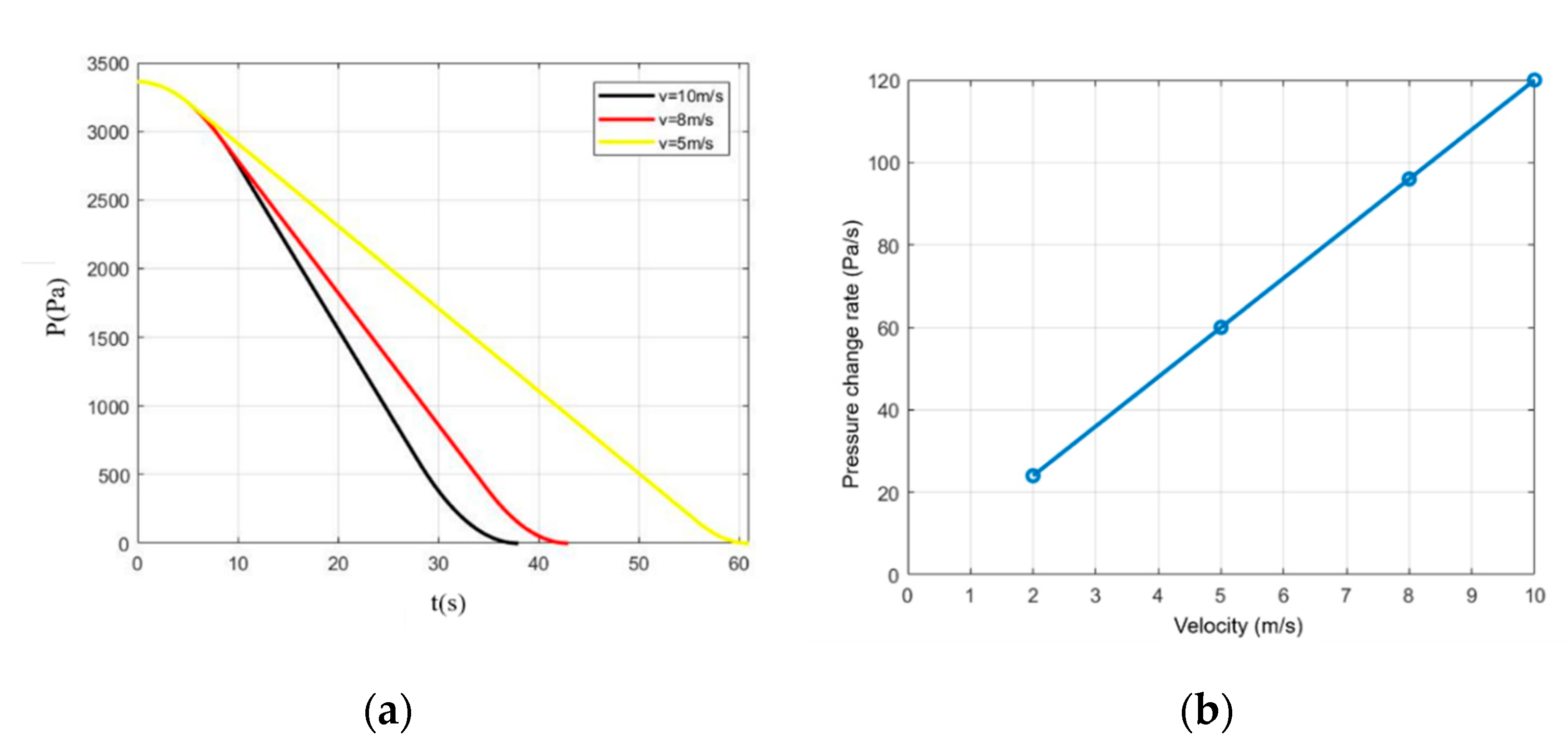
4.2. Multi-Factor Coupling Analysis of the Air Pressure Curves

To explore the influence of different parameters on the air pressure changes inside and outside the car, the air pressure changes inside and outside the KLK2 elevator car are analyzed under different operating parameters and the structure parameters of the IE-FF of the car. The numerical analysis is used to solve the law of air pressure changes inside and outside the car under different parameters. The specific simulation analysis process is shown in Figure 11. Ansys 2020/ICEM/CFD is utilized to mesh the model. The maximum element size meshed in the elevator car is 100 mm, the maximum element size meshed in the ventilation gap of car wall is 3 mm, the maximum element size meshed in the ventilation gap of car door is 3mm, the maximum element size meshed in the air inlet is 200 mm, the maximum element size meshed in the air outlet is 200 mm, and the maximum element size meshed in the hoistway wall is 200 mm. The boundary conditions of the elevator car and the hoistway walls are set as wall, boundary conditions of the car wall ventilation gap and car door ventilation gap are set as interior, and the boundary conditions of the air inlet is set as the velocity-inlet and the boundary conditions of the air outlet is set as pressure-inlet. The specific running parameters are set as is needed.

Based on the simulation analysis results, the influence of maximum running speed, running acceleration, lifting height, air leakage of the car, and speed of the fans of the ventilation system on the air pressure inside and outside the car is analyzed.

(1) The influence of elevator maximum running speed.

For traditional low-speed elevators, the maximum running speed will not have a large impact on the air pressure inside and outside the car since the airflow speed in the hoistway is small relative to the car. However, with the increase of elevator speed, the problem of elevator aerodynamic characteristics has gradually become prominent, and the air pressure distribution outside the car has become more and more complicated. As the speed of the elevator increases, the air pressure outside the car fluctuates between ±100 Pa, which is smaller than the low-speed elevators. The air pressure fluctuation outside the car will be transmitted to the inside of the car through the ventilation system and the leakage gap. According to numerical simulation, the influence of the elevator running speed on the air pressure inside and outside the car is shown in Figure 12. It can be seen that, when the overall lifting height of the elevator remains unchanged, the air pressure change amplitude caused by the speed increase is small, but it indirectly leads to an increase in the air pressure change rate, thus affecting the passenger ear comfort.

(2) The influence of elevator running acceleration.

By selecting three different elevator running accelerations, the relationship between the air pressure change inside and outside the car and the elevator acceleration is obtained, as shown in Figure 13. During the high-speed elevator operation, the air pressure change rate inside the car is not fixed. During the starting and braking of the elevator, the running acceleration also has an impact on the air pressure change inside the car, which directly affects the time for the air pressure change rate inside the car from slow to fast.

(3) The influence of elevator lifting height.

The elevator runs in a vertical shaft, and the distribution of atmospheric pressure in the vertical direction changes linearly. It can be seen from Figure 10b that the elevator lifting height directly affects the air pressure change inside and outside the car. The air pressure change amplitude that the human ear can withstand in a certain period of time is limited, so the elevator lifting height is the main factor that affects the air pressure change inside and outside the car.

(4) The influence of air leakage of the car.

Without considering the ventilation system, the air pressure fluctuation inside the car is mainly affected by the air leakage due to the gap. According to the gap flow model [35], the air leakage flow can be calculated:

$$q_{ml}=\frac{b{\delta }^3}{12\mu l}·\Delta p$$

(47)

where $\delta$. denotes the height of the gap, $b$ denotes the width of the gap,$l$ denotes the length of the gap, $\mu$ denotes the dynamic viscosity, and $\Delta p$ denotes the internal and external pressure difference.

The air pressure curve inside and outside the car is obtained by simulation, as shown in Figure 14. It can be seen that the air pressure curve outside the car reaches the target value before the air pressure curve inside the car for the same air pressure fluctuation and initial air pressure without the influence of the ventilation system. It reveals that the air pressure change inside the car has a pressure difference effect compared to the air pressure change outside the car due to the gap flow.

(5) The influence of speed of the fans in the ventilation system.

Figure 15 shows the flow characteristics of the fixed-speed fan. When the speed is constant, the fixed-speed fan works along its characteristic curve. When the external pressure decreases, the working point of the fixed-speed fan will move down along the characteristic curve, which will cause the air flow volume of the fan to change.

When the fixed-speed fans are applied in the ventilation system, in the case of continuous ventilation, the air pressure curve inside and outside the car is shown as Figure 16. It can be seen that, similar to the influence of the leakage gap, the air pressure change inside the car also has a pressure difference effect compared to the air pressure change outside the car.

4.3. Development of the Simulation Model

In order to verify the effectiveness of the elevator car air pressure compensation system, a KLK2 high-speed elevator is taken as an example to carry out the simulation analysis. The simulation-related parameters of KLK2 high-speed elevator are shown in

Table 3. Related parameters of the KLK2 elevator.

Parameter	Value
$\mathrm{Maximum} \mathrm{running} \mathrm{speed} \left(\mathrm{m}/\mathrm{s}\right)$	10.0
$\mathrm{Rated} \mathrm{load} \left(\mathrm{kg}\right)$	1600
$\mathrm{Area} \mathrm{of} \mathrm{the} \mathrm{car} \left({\mathrm{m}}^2\right)$	3.48
$\mathrm{Height} \mathrm{of} \mathrm{the} \mathrm{car} \left(\mathrm{mm}\right)$	2200
$\mathrm{Output} \mathrm{power} \mathrm{of} \mathrm{the} \mathrm{fan} \left(\mathrm{W}\right)$	1100
$\mathrm{Air} \mathrm{volume} \mathrm{of} \mathrm{the} \mathrm{fan} \left({\mathrm{m}}^3/\min \right)$	23
$\mathrm{Pressure} \mathrm{of} \mathrm{the} \mathrm{fan} (\mathrm{Pa})$	2100
$\mathrm{Speed} \mathrm{of} \mathrm{the} \mathrm{fan} \left(r/\min \right)$	2800

.

A simplified air pressure compensation system of the elevator car is set up in Matlab 2010b/Simulink. During the elevator operation, in order to take into account the air leakage, an extra fan is added to simulate the random external disturbance. The established model is shown in Figure 17.

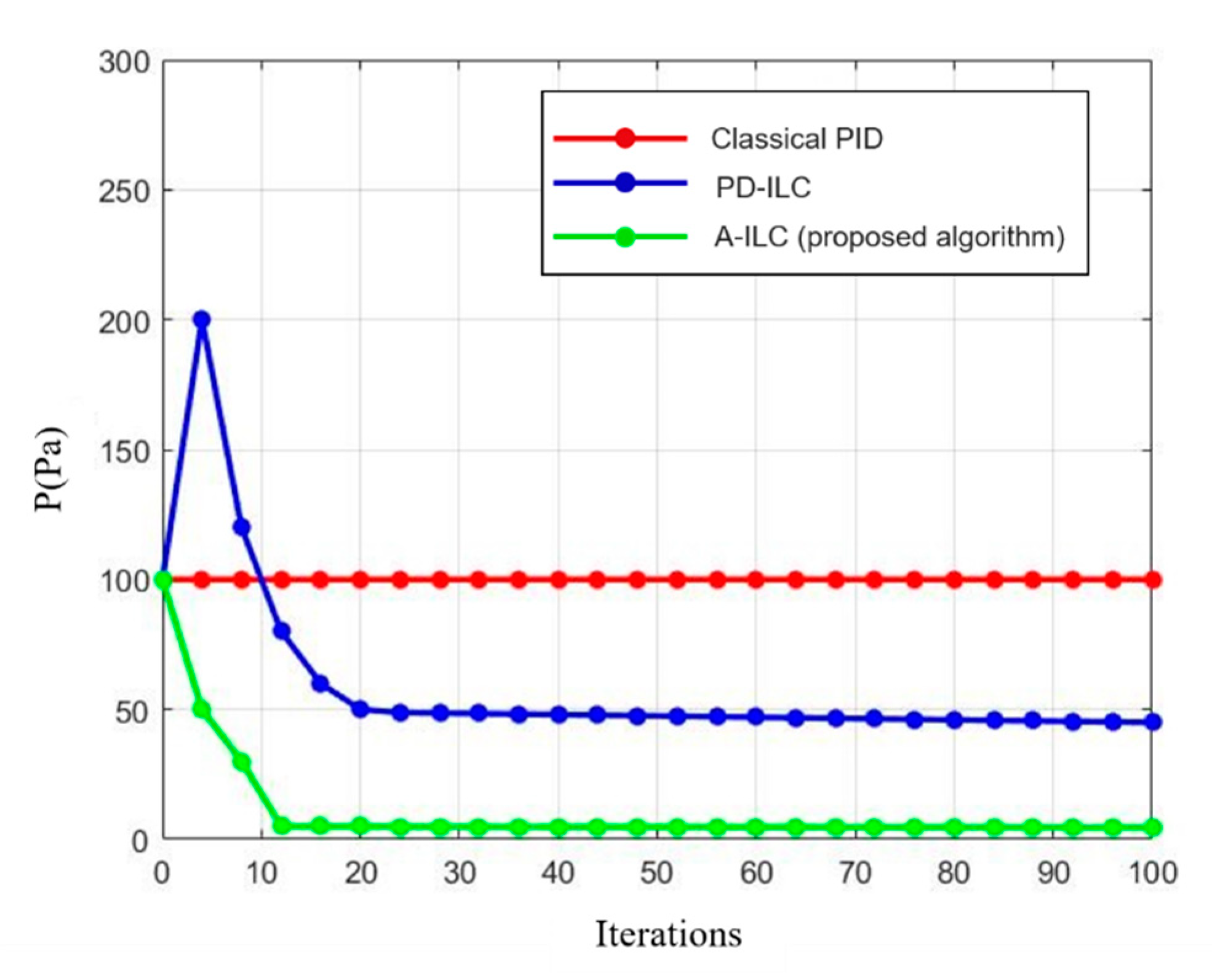
4.4. Results Comparison and Discussion

To verify the control accuracy of the proposed A-ILC algorithm for the air pressure compensation inside the car, the simulation results of the classical PID algorithm and the PD- ILC algorithm are selected for comparison.

The PID algorithm calculates the control error through the proportional term, integral term and derivative term to obtain the control input value at the next moment. In the simulation experiments, the gain coefficients of the proportional term, integral term and differential term are set to 2, 0.8 and 0.2, respectively. The controller of the PD-ILC algorithm is given by Equation (29). The controller of the proposed A-ILC algorithm is given by Equation (46).

The IAPC inside the car is used as the target curve to compare the accuracy of the three algorithms. The air pressure compensation results of PID, PD-ILC and the proposed A-ILC are shown in Figure 18. It can be seen that the three control algorithms have good tracking effects on the target curve on the entire time axis. However, when the target curve changes suddenly, the control effects of the three algorithms are different at the air pressure inflection point. As the PID algorithm predicts the control input at the next time based on the tracking error at the previous time, the air pressure compensation will deviate from the target curve when the target value changes greatly. However, the tracking accuracy of ILC algorithm and A-ILC algorithm based on the iterative learning principle will become higher and higher as the number of iterations increase.

The air pressure tracking errors of the classical PID algorithm, the PD-ILC algorithm and the proposed A-ILC algorithm are shown in Figure 19. In this figure, the ordinate is the root mean square value of the tracking error in the total time of compensation and control. As can be seen from this figure, due to the lack of a learning mechanism in the spatial domain for PID algorithm, the tracking error always maintains a high value; and compared with the A-ILC algorithm, the PD-ILC algorithm has lower tracking accuracy and slower convergence speed.

5. Conclusions

To improve the ride comfort of the high-speed elevator, an air pressure compensation method was proposed to actively compensate and adjust the air pressure inside the elevator car, which can effectively eliminate the passengers’ ear pressing due to the severe air pressure fluctuation. The conclusions are as follows:

(1)

During the operation of the high-speed elevator, the severe air pressure fluctuation outside the car will affect the air pressure inside the car. To realize the accurate compensation of the air pressure inside the car, the IE-FF coupling variation model was established to accurately obtain the transient air pressure change inside the car. Based on this model, the variation amplitude and trend of the air pressure curve inside the car obtained by iterative calculations was consistent with the measurement.

(2)

The influence of different factors on the air pressure inside and outside the car was investigated. Results showed that the maximum running speed, running acceleration and lifting height of the high-speed elevator had a great influence on both the air pressure inside and outside the car. Due to the air leakage gap and the ventilation system, the air pressure change inside the car had a pressure difference effect compared to that outside the car.

(3)

To verify the effectiveness of the air pressure compensation method, the numerical experiments were carried out through Matlab/Simulink. Taking the KLK2 high-speed elevator as an example, the results showed that the tracking accuracy and convergence speed of the A-ILC algorithm were better than the classical PID algorithm and the ILC algorithm. When the air pressure changed greatly, the air pressure compensation would deviate from the IAPC, and the ILC and A-ILC algorithms would have higher and higher tracking accuracy as the number of iterations increased.

References

1. Ding, B.; Zhang, Y.M.; Peng, X.Y.; Li, Q.C.; Tang, H.Y. A hybrid approach for the analysis and prediction of elevator passenger flow in an office building. Autom. Constr. 2013, 35, 69–78. [Google Scholar] [CrossRef]
2. Qiu, L.M.; Zhou, H.F.; Wang, Z.L.; Lou, W.Q.; Zhang, S.Y.; Zhang, L.C. A Stepped-Segmentation Method for the High-Speed Theoretical Elevator Car Air Pressure Curve Adjustment. Energies 2020, 13, 2585. [Google Scholar] [CrossRef]
3. Duan, Y.; Shen, G.; Zhang, Y.; Su, W. Aerodynamic testing simulation facility for high-speed elevator. J. Beijing Univ. Aeronaut. Astronaut. 2004, 30, 444–447. [Google Scholar]
4. Zhu, W.D.; Teppo, L.J. Design and analysis of a scaled model of a high-rise, high-speed elevator. J. Sound Vib. 2003, 264, 707–731. [Google Scholar] [CrossRef]
5. Bai, H.L.; Shen, G.X.; So, A. Experimental-based study of the aerodynamics of super-high-speed elevators. Build. Serv. Eng. Res. Technol. 2005, 26, 129–143. [Google Scholar] [CrossRef]
6. Matsuda, H. Cause and Modification of the Aerodynamic Noise on High Speed Elevator. J. INCE Jpn. 1994, 18, 32–36. [Google Scholar]
7. Matsuda, H.; Fukuyama, Y.; Yokono, Y.; Miyasaku, K. The Effect of Car Configurations on the Flow Around Elevator Models (Oil Flow Pattern and Distribution of Pressure Fluctuation on the Model Wall Surface). In Flow Visualization VI; Tanida, Y., Miyashiro, H., Eds.; Springer: Berlin/Heidelberg, Germany, 1992; pp. 275–279. [Google Scholar]
8. Wang, X.B.; Lin, Z.; Tang, P.; Lin, Z.W. Research of the blockage ratio on the aerodynamic performances of high speed elevator. In Proceedings of the 2015 4th International Conference on Mechatronics, Materials, Chemistry and Computer Engineering, Xi’an, China, 12–13 December 2015; Atlantis Press: Xi’an, China, 2015. [Google Scholar]
9. Shi, L.Q.; Liu, Y.Z.; Jin, S.Y.; Cao, Z.M. Numerical simulation of unsteady turbulent flow induced by two-dimensional elevator car and counter weight system. J. Hydrodyn. Ser. B 2007, 19, 720–725. [Google Scholar] [CrossRef]
10. Mei, D.Q.; Du, X.Q.; Chen, Z. Optimization of dynamic parameters for a traction-type passenger elevator using a dynamic byte coding genetic algorithm. Proc. Inst. Mech. Eng. Part C 2009, 223, 595–605. [Google Scholar] [CrossRef]
11. Hara, T. Aerodynamic Force Acting on a High Speed Train at Tunnel Entrance. Bull. JSME 1961, 4, 547–553. [Google Scholar] [CrossRef] [Green Version]
12. Vardy, A.E. Generation and alleviation of sonic booms from rail tunnels. Eng. Comput. Mech. 2008, 161, 107–119. [Google Scholar] [CrossRef]
13. Sockel, H. Aerodynamic effects caused by a train entering a tunnel. PAMM 2002, 1, 268–269. [Google Scholar] [CrossRef]
14. Sockel, H. Formulae for the calculation of pressure effects in railway tunnels. Int. Symp. Aerodyn. Vent. Vehicle Tunn. 2003, 2, 581–595. [Google Scholar]
15. Anthoine, J. Alleviation of Pressure Rise from a High-Speed Train Entering a Tunnel. AIAA J. 2009, 47, 2132–2142. [Google Scholar] [CrossRef]
16. Biotto, C.; Proverbio, A.; Ajewole, O.; Waterson, N.; Peiro, J. On the treatment of transient area variation in 1D discontinuous Galerkin simulations of train-induced pressure waves in tunnels. Int. J. Numer. Methods Fluids 2013, 71, 151–174. [Google Scholar] [CrossRef]
17. Yoon, T.; Lee, S. Efficient prediction methods for the micro-pressure wave from a high-speed train entering a tunnel using the Kirchhoff formulation. J. Acoust. Soc. Am. 2001, 110, 2379–2389. [Google Scholar] [CrossRef] [PubMed] [Green Version]
18. Klaver, E.C.; Kassies, E. Dimensioning of tunnels for Passenger comfort in Netherlands. In Proceedings of the 10th International Symposium on the Aerodynamics and Ventilation of Vehicle Tunnels, Boston, MA, USA, 1–3 November 2000; BHR Group: Cranfield, UK, 2000; pp. 737–755. [Google Scholar]
19. Schwanitz, S.; Wittkowski, M.; Rolny, V.; Basner, M. Pressure variations on a train—Where is the threshold to railway passenger discomfort? Appl. Ergon. 2013, 44, 200–209. [Google Scholar] [CrossRef]
20. Schwanitz, S.; Wittkowski, M.; Rolny, V.; Samel, C.; Basner, M. Continuous assessments of pressure comfort on a train—A field-laboratory comparison. Appl. Ergon. 2013, 44, 11–17. [Google Scholar] [CrossRef] [PubMed]
21. Sanz-Andrés, A.; Santiago-Prowald, J. Train-induced pressure on pedestrians. J. Wind Eng. Ind. Aerodyn. 2002, 90, 1007–1015. [Google Scholar] [CrossRef] [Green Version]
22. Lei, Y.; Ye, Y.; Chen, Z. Horizontal wind effect on the aerodynamic performance of coaxial Tri-Rotor MAV. Appl. Sci. 2020, 10, 8612. [Google Scholar] [CrossRef]
23. Yamamoto, K. Elevator Control Device and Elevator Device. Japan Patent 102066223, 18 May 2011. [Google Scholar]
24. Yangyou, K.; Shi, W. Control Method of Internal Pressure of Elevator Car. Japan Patent 106081766, 9 November 2016. [Google Scholar]
25. Mizuno, S.; Fujita, Y.; Togashi, N.; Kaida, Y. The development of air pressure control system for elevator cage. In Proceedings of the Elevator Escalator and Amusement Rides Conference 2004, Tokyo, Japan, 14–16 June 2004; Volume 2, pp. 21–24. [Google Scholar]
26. Zhang, Y.; Su, J.; Chen, M. Research on Adaptive Iterative Learning Control of Air Pressure in Railway Tunnel with IOTs Data. IEEE Access 2020, 8, 5481–5487. [Google Scholar] [CrossRef]
27. Hou, X.M.; Zhang, X.J. The Simulation Research on Pressure Control System of the High-Speed Train’s Carriage. Appl. Mech. Mater. 2011, 120, 547–550. [Google Scholar] [CrossRef]
28. Li, X.; Chen, C.J. Active-passive control of internal pressure of high-speed train based on fuzzy PID. China Meas. Test 2020, 46, 105–109. [Google Scholar]
29. Lumley, J.L. Computational modeling of turbulent flows. Adv. Appl. Mech. 1979, 18, 123–176. [Google Scholar]
30. Alfonsi, G. Reynolds-Averaged Navier–Stokes equations for turbulence modeling. Appl. Mech. Rev. 2009, 62, 040802. [Google Scholar] [CrossRef]
31. Matsson, J. An Introduction to ANSYS Fluent 2020; SDC Publications: Ulaanbaatar, Mongolia, 2020. [Google Scholar]
32. Von Bernuth, R.D. Simple and accurate friction loss equation for plastic pipe. J. Irrig. Drain. E-ASCE 1990, 116, 294–297. [Google Scholar] [CrossRef]
33. Bristow, D.A.; Tharayil, M.; Alleyne, A.G. A survey of iterative learning control. IEEE Contr. Syst. Mag. 2006, 26, 96–114. [Google Scholar]
34. Owens, D.H.; Hätönen, J. Iterative learning control—An optimization paradigm. Annu. Rev. Control 2005, 29, 57–70. [Google Scholar] [CrossRef]
35. Sasa, G. The dynamics of gap flow over idealized topography. Diss. Abstr. Int. 2002, 2, 1233–1244. [Google Scholar]
Figure 1. Coupling characteristic of the IE-FF of the car (rotated 90°).
Applsci 11 01700 g001
Figure 2. Calculation process of the transient coupling.
Applsci 11 01700 g002
Figure 3. The structure of the air pressure compensation system with double fans. 1—Control device, 2,3—Frequency converter, 4,7—Filter, 5—Pressurizing fan, 6—Decompressing fan, 8—Elevator car, 9—Barometer.
Applsci 11 01700 g003
Figure 4. The dual-fan air pressure compensation system with a feedback link.
Applsci 11 01700 g004
Figure 5. The general flow characteristic curve of the fan.
Applsci 11 01700 g005
Figure 6. Iterative learning principle of ILC.
Applsci 11 01700 g006
Figure 7. PD-ILC controller of the air pressure compensation system.
Applsci 11 01700 g007
Figure 8. A-ILC system for the air pressure compensation system.
Applsci 11 01700 g008
Figure 9. Experimental instruments. (a) 288 m elevator test tower in Canny; (b) ZOGLAB DSR-THP temperature, humidity and pressure recorder; and (c) PMT-EVA625 elevator comprehensive performance tester.
Applsci 11 01700 g009
Figure 10. Air pressure value curves (measured by experiments) inside the elevator car. (a) At the same height ( H = 217 m ) and different speeds; and (b) at the same speed ( v = 10 m / s ) and different heights.
Applsci 11 01700 g010
Figure 11. Simulation analysis process of the air pressure change inside and outside the car.
Applsci 11 01700 g011
Figure 12. Influence of the elevator running speed on the air pressure change inside the car. (a) On the air pressure change value amplitude. (b) On the air pressure change rate.
Applsci 11 01700 g012
Figure 13. Influence of elevator running acceleration on the air pressure change value inside the car.
Applsci 11 01700 g013
Figure 14. Air pressure change value curves inside and outside the car without the ventilation system.
Applsci 11 01700 g014
Figure 15. Characteristic curves of the fans.
Applsci 11 01700 g015
Figure 16. Air pressure change value curves inside and outside the car under continuous ventilation.
Applsci 11 01700 g016
Figure 17. Simulation model of the high-speed elevator car air pressure compensation system.
Applsci 11 01700 g017
Figure 18. Comparison of the air pressure compensation methods.
Applsci 11 01700 g018
Figure 19. Comparison of the air pressure tracking error inside the car.
Applsci 11 01700 g019