Application of Artificial Intelligence to Determined Unconfined Compressive Strength of Cement-Stabilized Soil in Vietnam

Abstract

Cement stabilized soil is one of the commonly used as ground reinforcement solutions in geotechnical engineering. In this study, the main object was to apply three machine learning (ML) methods namely gradient boosting (GB), artificial neural network (ANN) and support vector machine (SVM) to predict unconfined compressive strength (UCS) of cement stabilized soil. Soil samples were collected at Hai Duong city, Vietnam. A total of 216 soil–cement samples were mixed in the laboratory and compressed to determine the UCS. This data set is divided into two parts of the training data set (80%) and testing set (20%) to build and test the model, respectively. To verify the performance of ML model, various criteria named correlation coefficient (R), mean absolute error (MAE) and root mean square error (RMSE) were used. The results show that all three ML models were effective methods to predict the UCS of cement-stabilized soil. Amongst three model used in this study, optimized ANN model provided superior performance compare to two others models with performance indicator R = 0.925, RMSE = 419.82 and MAE = 292.2 for testing part. This study can provide an effective tool to quickly predict the UCS of cement stabilized soil with high accuracy.

1. Introduction

Ground under the foundation is an important part, which has the effect of bearing most or all of the load on the building. The presence of soft soil layers under the foundation can cause problems for buildings [1]. However, in recent decades, the urban population is increasing rapidly, increasing the need for infrastructure, so soft ground areas are also studied for the construction of buildings. These soils are often characterized by high plasticity, high void ratio and low strength [2]. Soft soil can be reinforced by various methods depending on specific conditions [3], such as mechanically stabilized earth (MSE) embankments [4], granular or sand compaction piles [5], vertical drains [6] and the lime/cement deep mixing method [7]. In another study, YI Oh and EC Shin used pile reinforcement revetments and ground net reinforcement on soft ground to reduce deflection settlement [8]. Among the soft soil reinforcement methods, the cement-stabilized sandy soil method has been used for many years [9,10]. The cementation of sandy soil can increase the hardness, shear strength and compressive strength of the material [9]. Many researchers have investigated the mechanical properties of cement-treated soil by various methods. For example, Changizi and Haddad [11] ran a series of unconfined compression tests and direct shear tests, their studies have shown that the unconfined compressive strength (UCS) and soil adhesion will increase when the nanosilica content increases. In addition, using the unconfined compression tests and the California bearing ratio (CBR) tests, Ghasabkolaei et al. [12] and Choobbasti et al. [13] also concluded similarly about the positive relationship between UCS value and nanosilica content that is in the composition of cement. In many other studies, the authors also build experimental models to predict the strength of cement stabilized soft ground [14].

Based on the experimental results, Miura et al. [15] gave the experimental equations to calculate UCS of high water content cement stabilized clay based on the ratio of cement and water. In addition, Horpibulsuk et al. [16] have developed a standardized experimental model to predict cement stabilized soil strength based on Abram’s law, and at the same time consider the cement–water ratio as the main parameter. Last but not least, a model equation to calculate the cement content required to reach a desired strength, which scientist Horpibulsuk et al. [17] have drawn from the results of experiments on soft clay mixed cement and considering the ratio of water–cement is a microstructural parameter.

Through many studies it can be found that the UCS value is an important parameter to evaluate the bearing capacity of cement-stabilized soil [3,9]. However, the UCS value is mainly determined by experimental studies and experimental equations. However, the experimental method often requires a large number of samples, it is expensive and time-consuming [18]. Moreover, the experimental equations often have to be based on approximate hypotheses, so errors still exist [16]. In addition, the soil properties in each place are so different, it is difficult to apply the general experimental formulas.

In recent years, artificial intelligence and machine learning models are used more and more widely, many scientists in the field of geology apply these models to predict the UCS value of soil stabilized with cement. Of particular note is the study of Narendra et al. [19]. They built a genetic programming model GP to predict the UCS value of red earth (CL), brown earth (CH) and black cotton soil (CH) stabilized with cement. In addition, the algorithms ANN and SVM are also used to predict unconfined compressive strength of cement stabilized soil [18,20] these models show high accuracy, and cost savings compared to experimental methods [18].

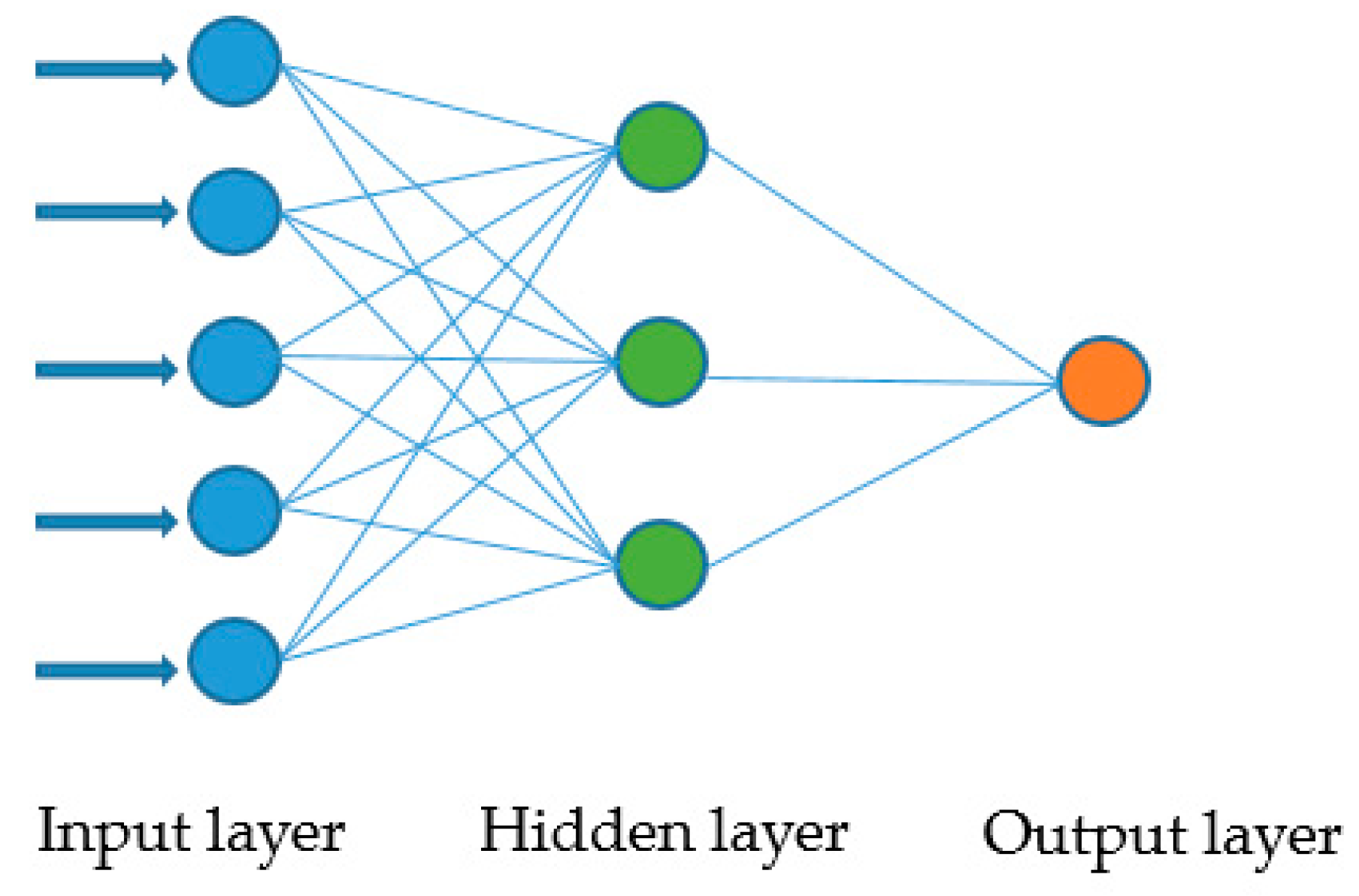
In this study, the main object is to apply three machine learning (ML) methods namely gradient boosting (GB), artificial neural network (ANN) and support vector machine (SVM) to predict unconfined compressive strength of cement stabilized soil. The model architectures were optimized then using the Monte-Carlo method to model and consider the randomness of the data division. To verify the performance of the ML model, different criteria named correlation coefficient (R), mean absolute error (MAE) and root mean square error (RMSE) were used. The results show that the optimized ML models are an efficient and stable method to predict the unlimited compressive strength of soil–cement mixing piles.

2. Significance of the Research Study

Accurately predicting the UCS of cement-stabilized soil is of crucial important because of many possible advantages and contributions to foundation reinforcement. Approaches in the available literature still face some limitations, for instance, the lack of dataset samples (Suman et al. [18] with 58 samples; Das et al. [20] with 55 samples and Hoang-Anh Le et al. [21] with 118 samples), accuracy assessment and improvement of the ML approaches. Therefore, the contribution of the present study could be highlighted through the following ideas: (i) an unpublished large data set include 216 experimental tests; (ii) a comparison of 3 ML algorithms, namely GB, ANN and SVR, which model architectures were optimized using random search technique; (iii) the performance of ML algorithms is evaluated under the presence of random splitting dataset, which could truly find out the efficiency of ML algorithms and (iv) a sensitivity analysis is performed to reveal the role of each input parameters in predicting the UCS of cement-stabilized soil.

3. Data Collection and Preparation

3.1. Experimental Measurement of UCS of Cement-Stabilized Soil

In this study, a database containing 216 soil samples were collected at Tran Nguyen Han street, Thanh Binh district, Hai Duong city, Vietnam (Figure 1). Soil samples were collected at two −2.0 m and −4.0 m depth, in three boreholes. Those boreholes were made with 10 m distance from each other. Soil samples were collected by pressing a cylinder into the soil block at the boreholes, and then covered with a moisture-proof bag to keep original water content (Figure 2). Collected soil were stored and transported by boxcar from the collecting site to the laboratory.

Soil parameters was analyzed, evaluated and processed through specific stages: moisture content tests; wet density tests; mix soil cement; forming and curing of specimen and then unconfined compression tests were performed using specialized equipment (Figure 3). Experimental results obtained the relationship of axial stress–strain curves (Figure 4) and the UCS of the samples were defined as destructive compressive axial stress. An example of axial stress–strain curves are given in Appendix B (Figure A1).

It is important to note that three kinds of general cement in the north of Vietnam were used for the cement mixing test, including Vissai cement, Chinfon Hai Phong cement and Nghi Son cement. A cement mixing ratio (i.e., the amount of cement in q m³ of the mixture) was applied to 100 kg/m³, 150 kg/m³ and 200 kg/m³. The specimens were cured during 7 days and 28 days at the indoor and outdoor condition. With the indoor curing condition, the specimens were covered with a sealant to prevent water evaporation from the specimen and the specimen was placed in the curing container. On the other hand, outdoor curing of specimens were placed in a room without any controlled intern of temperature and humidity, and without the sealant.

3.2. Data Preparation

It is known that the UCS values depend on a large number of parameters. In this study, factors that are important in the UCS of the soil–cement mixture determination were selected. The soil type (denoted as S) seem to influence the UCS of the mixture as it determines the soil’s grain composition [22]. Moisture content of soil samples (denoted as Mc) also play an important role in the UCS detecting [23,24]. The wet density of soil (denoted as We) should also be considered as it determines the natural state of the soil prior to mixing [24]. The soil sampling depth (denoted as D) should also be taken into account when it affects the soil condition [25]. We cannot fail to mention the amount of cement (denoted as Ac) used for mixing when it determines the adhesion between soil particles [26]. Factors related to the sample after mixing such as: specimen diameter (denoted as Di); specimen length (denoted as L); specimen area (denoted as A); specimen volume (denoted as V); mass of specimen (denoted as M) and density of specimen (denoted as De) might also affect much to the prediction [27,28]. In addition, a number of other important factors to consider were the curing condition (denoted as Cc) and the curing period (denoted as Cp) that affect the rate of strength development of the cement. Finally, the type of cement (denoted as T) was also taken into consideration when the quality of cement in Vietnam appears to be uneven among each other. The UCS of the cement–soil mixture (denoted as q_u) was the single output. Detailed statistics of the parameters used in the study are presented in

Table 1. Inputs and output of the present study.

No	D	We	Cc (*)	Cp	S (*)	Mc	T (*)	Ac	Di	L	A	V	M	De	qu
Unit	m	g/cm3	-	-	-	%	-	kg/cm3	cm	cm	cm2	cm3	g	g/cm3	kPa
1	4	1.72	1	7	2	1.72	1	100	4	10	19.4	194	339.8	1.75	472
2	4	1.76	1	7	3	1.76	1	100	5	10	19.45	194.52	333.8	1.72	498.2
3	4	1.72	1	7	2	1.72	1	100	5	10	19.63	196.35	342	1.74	649.41
.	.	.	.	.	.	.	.	.	.	.	.	.	.	.	.
.	.	.	.	.	.	.	.	.	.	.	.	.	.	.	.
.	.	.	.	.	.	.	.	.	.	.	.	.	.	.	.
214	2	1.93	2	28	1	1.96	2	200	5	10	19.43	194.26	324.4	1.67	3780.35
215	2	1.93	2	28	1	1.93	2	200	5	10	19.4	194	317.8	1.64	4143.8
216	2	1.93	2	28	1	1.9	2	200	4.9	10	19.17	191.67	324.2	1.69	4922.67
Min	2.00	1.72	1.00	7.00	1.00	1.72	1	100	4.00	10	18.86	188.57	248.80	1.31	244.06
Average	3.00	1.83	1.50	17.50	1.67	1.83	2	150	4.98	10	19.48	194.87	336.31	1.72	1927.87
Max	4.00	1.93	2.00	28.00	3.00	1.96	3	200	5.00	10	19.74	197.40	385.80	1.96	5129.83
SD (*)	1.00	0.10	0.50	10.52	0.75	0.10	0.82	40.92	0.07	0.00	0.19	1.96	36.26	0.18	1215.94

SD ⁽*⁾ = Standard deviation; Cc ⁽*⁾: 1—Indoor; 2—outdoor; S ⁽*⁾: 1—Yellow clay; 2—Black organic sandy clay; 3—Black sandy clay; T ⁽*⁾: 1—Vissai cement; 2—Nghi Son cement; 3—Chinfon Hai Phong cement.

. An example of this data set is given in Appendix A (

Table A1. An example of the data set of the present study.

No	D	We	Cc	Cp	S	Mc	T	Ac	Di	L	A	V	M	De	qu
Unit	m	g/cm3	-	-	-	%	-	kg/cm3	cm	cm	cm2	cm3	g	g/cm3	kPa
1	2	1.93	1	7	1	1.9	1	150	5	10	19.63	196.35	379.8	1.93	1707.95
2	2	1.93	2	7	1	1.93	2	200	5	10	19.37	193.74	342.2	1.77	4018.33
3	4	1.72	2	28	2	1.72	3	200	5	10	19.48	194.78	278	1.43	2336.29
4	2	1.93	1	28	1	1.96	1	100	5	10	19.63	196.35	381.4	1.94	1836.64
5	4	1.72	2	7	2	1.72	3	150	5	10	19.32	193.22	309	1.6	1383.56
6	2	1.93	1	7	1	1.93	1	200	5	10	19.63	196.35	377.2	1.92	1976.48
7	4	1.76	2	28	3	1.76	2	200	5	10	19.45	194.52	274.2	1.41	3147.3
8	2	1.93	2	28	1	1.9	2	200	4.9	10	19.17	191.67	324.2	1.69	4922.67
9	2	1.93	1	7	1	1.96	2	100	5	10	19.63	196.35	375.2	1.91	791.39
10	2	1.93	2	28	1	1.96	3	100	4.9	10	19.01	190.12	300	1.58	1118.24
11	4	1.72	2	7	2	1.72	3	200	5	10	19.58	195.83	313.6	1.6	1475.3
12	4	1.76	1	28	3	1.76	1	150	5	10	19.63	196.35	349.2	1.78	1363.25
13	4	1.72	1	7	2	1.72	1	150	5	10	19.63	196.35	346.4	1.76	805.39
14	2	1.93	1	7	1	1.93	2	150	5	10	19.63	196.35	375.4	1.91	1422.7
15	2	1.93	1	28	1	1.9	3	100	5	10	19.63	196.35	379	1.93	695.1
16	2	1.93	1	28	1	1.93	3	100	5	10	19.63	196.35	380.4	1.94	755.31
17	2	1.93	1	7	1	1.9	2	100	5	10	19.63	196.35	379	1.93	1158.82
18	2	1.93	2	7	1	1.96	3	100	5	10	19.48	194.78	331	1.7	1289.44
19	4	1.72	1	28	2	1.72	2	100	5	10	19.63	196.35	354.6	1.81	449.55
20	2	1.93	1	7	1	1.9	2	150	5	10	19.63	196.35	382.4	1.95	1799
21	4	1.72	1	28	2	1.72	1	150	5	10	19.63	196.35	355.8	1.81	1105.88
22	2	1.93	2	7	1	1.93	1	200	5	10	19.43	194.26	346	1.78	4099.15
23	2	1.93	1	28	1	1.96	1	200	5	10	19.63	196.35	379.6	1.93	2596.24
24	2	1.93	1	28	1	1.93	2	200	5	10	19.63	196.35	382.4	1.95	2619.07
25	4	1.72	2	7	2	1.72	1	100	4.9	10	19.17	191.67	311.4	1.62	900.82
26	4	1.76	2	28	3	1.76	2	150	5	10	19.32	193.22	267.8	1.39	2238.02
27	2	1.93	1	28	1	1.9	2	150	5	10	19.63	196.35	382.8	1.95	2734.99
28	4	1.76	1	7	3	1.76	1	100	5	10	19.45	194.52	333.8	1.72	498.2
29	4	1.76	2	7	3	1.76	3	150	5	10	19.43	194.26	310.4	1.6	1995.69
30	2	1.93	1	28	1	1.9	2	100	5	10	19.63	196.35	378.2	1.93	1883.47
31	2	1.93	1	28	1	1.96	3	100	5	10	19.63	196.35	376.2	1.92	499.66
32	4	1.76	2	7	3	1.76	3	200	5	10	19.48	194.78	313.4	1.61	2305.96
33	4	1.76	2	28	3	1.76	3	150	4.9	10	19.06	190.63	262.4	1.38	1909.18
34	2	1.93	2	28	1	1.93	1	150	5	10	19.3	192.96	311.2	1.61	4595.34
35	2	1.93	1	28	1	1.96	1	150	5	10	19.63	196.35	377.2	1.92	1936.14
36	4	1.76	2	28	3	1.76	1	100	4.9	10	18.86	188.57	255.6	1.36	713.58
37	2	1.93	1	7	1	1.96	1	200	5	10	19.53	195.3	376.8	1.93	1316.62
38	2	1.93	1	28	1	1.9	2	200	5	10	19.63	196.35	382.4	1.95	3076.98
39	4	1.72	2	28	2	1.72	2	100	4.9	10	18.93	189.34	257.8	1.36	687.38
40	4	1.72	1	28	2	1.72	2	150	5	10	19.63	196.35	350.6	1.79	710.01
41	4	1.72	1	28	2	1.72	1	200	5	10	19.63	196.35	355.4	1.81	1690.15
42	4	1.76	1	28	3	1.76	3	100	5	10	19.63	196.35	346.6	1.77	605.68
43	2	1.93	1	7	1	1.96	2	200	5	10	19.63	196.35	384.4	1.96	1744.79
44	2	1.93	1	28	1	1.96	3	200	5	10	19.63	196.35	383.4	1.95	2705.26
45	4	1.72	2	7	2	1.72	2	100	5	10	19.43	194.26	298.2	1.54	660.47
46	2	1.93	1	7	1	1.9	2	200	5	10	19.63	196.35	385.8	1.96	1992.59
47	2	1.93	2	28	1	1.96	2	100	5	10	19.22	192.18	301.6	1.57	2725.33
48	2	1.93	2	28	1	1.93	2	200	5	10	19.4	194	317.8	1.64	4143.8
49	2	1.93	1	28	1	1.93	3	150	5	10	19.63	196.35	380.2	1.94	2396.77
50	2	1.93	2	7	1	1.93	3	150	5	10	19.32	193.22	356	1.84	3197.18
51	4	1.72	2	7	2	1.72	3	200	5	10	19.48	194.78	313.4	1.61	2305.96
52	4	1.76	2	7	3	1.76	1	150	5	10	19.45	194.52	324.8	1.67	1223.71
53	2	1.93	2	28	1	1.9	1	200	5	10	19.3	192.96	319.6	1.66	5129.83
54	2	1.93	2	28	1	1.93	3	150	5	10	19.3	192.96	311	1.61	4864.9
55	4	1.76	1	28	3	1.76	2	150	5	10	19.63	196.35	352.8	1.8	1352.47
56	4	1.72	2	7	2	1.72	3	150	5	10	19.43	194.26	313.8	1.62	1067.63
57	2	1.93	2	28	1	1.96	3	150	4.9	10	19.11	191.15	309.6	1.62	4085.39
58	4	1.76	2	28	3	1.76	3	200	5	10	19.24	192.44	275.6	1.43	3856.02
59	4	1.72	2	7	2	1.72	2	150	5	10	19.63	196.35	301.4	1.54	998.22
60	4	1.72	2	28	2	1.72	2	200	5	10	19.45	194.52	275.4	1.42	2080.09
61	4	1.72	2	7	2	1.72	2	200	5	10	19.69	196.87	303.2	1.54	1889.58
62	2	1.93	1	7	1	1.93	3	200	5	10	19.63	196.35	377.6	1.92	1702.19
63	4	1.72	2	28	2	1.72	3	200	5	10	19.32	193.22	277.8	1.44	2481.45
64	2	1.93	2	7	1	1.9	1	200	5	10	19.19	191.92	346.6	1.81	4149.05
65	2	1.93	1	7	1	1.93	1	100	5	10	19.63	196.35	376.2	1.92	1192.32
66	2	1.93	1	28	1	1.96	3	150	5	10	19.63	196.35	380.2	1.94	1982.46
67	2	1.93	1	28	1	1.96	2	100	5	10	19.63	196.35	376	1.91	1215.35
68	4	1.76	1	7	3	1.76	2	150	5	10	19.63	196.35	350	1.78	754.49
69	2	1.93	1	28	1	1.93	3	200	5	10	19.63	196.35	380.4	1.94	2470.45
70	2	1.93	2	28	1	1.96	1	200	5	10	19.43	194.26	315.6	1.62	3906.32
71	4	1.72	1	28	2	1.72	3	100	5	10	19.63	196.35	341.6	1.74	568.93
72	4	1.72	1	28	2	1.72	2	100	5	10	19.63	196.35	350.6	1.79	418.33
73	4	1.72	1	7	2	1.72	3	100	5	10	19.63	196.35	342	1.74	298.24
74	4	1.72	1	28	2	1.72	2	200	5	10	19.63	196.35	354.6	1.81	1232.07
75	4	1.72	2	7	2	1.72	2	150	5	10	19.63	196.35	311	1.58	1103.77
76	4	1.72	2	7	2	1.72	1	150	5	10	19.53	195.3	322.2	1.65	1193.45
77	2	1.93	2	28	1	1.9	3	150	4.9	10	19.11	191.15	312.4	1.63	3882.56
78	2	1.93	2	7	1	1.93	3	100	5	10	19.32	193.22	343	1.78	1562.15
79	4	1.72	2	7	2	1.72	3	100	5	10	19.27	192.7	282.2	1.46	990.67
80	4	1.72	2	28	2	1.72	2	200	5	10	19.4	194	276.4	1.42	2221.06
81	4	1.76	1	7	3	1.76	2	200	5	10	19.63	196.35	355.4	1.81	1138.63
82	2	1.93	2	28	1	1.93	3	100	5	10	19.24	192.44	305.8	1.59	1560.77
83	2	1.93	2	28	1	1.93	2	150	5	10	19.24	192.44	305.2	1.59	4363.29
84	4	1.72	2	7	2	1.72	1	200	5	10	19.74	197.4	312	1.58	1621.66
85	2	1.93	2	7	1	1.93	1	100	5	10	19.27	192.7	336.6	1.75	1857.65
86	4	1.72	1	28	2	1.72	2	200	5	10	19.63	196.35	358	1.82	1393.78
87	4	1.72	1	7	2	1.72	1	200	5	10	19.63	196.35	349.4	1.78	1311
88	4	1.76	1	7	3	1.76	3	150	5	10	19.63	196.35	342.2	1.74	765.61
89	2	1.93	2	7	1	1.93	2	100	5	10	19.35	193.48	337.8	1.75	3019.78
90	2	1.93	2	28	1	1.9	2	150	4.9	10	19.01	190.12	318	1.67	4785.22
91	4	1.72	1	28	2	1.72	3	200	5	10	19.63	196.35	357.8	1.82	1642.09
92	4	1.72	2	7	2	1.72	1	100	5	10	19.37	193.74	293	1.51	807.75
93	2	1.93	1	7	1	1.96	3	150	5	10	19.63	196.35	379	1.93	1648.09
94	2	1.93	2	7	1	1.96	1	200	5	10	19.45	194.52	345.4	1.78	2821.29
95	2	1.93	1	28	1	1.93	1	150	5	10	19.63	196.35	379.6	1.93	2454.92
96	2	1.93	2	7	1	1.93	3	200	5	10	19.48	194.78	351.4	1.8	3222.19
97	4	1.72	2	7	2	1.72	2	200	5	10	19.66	196.61	294.8	1.5	1907.62
98	4	1.72	1	7	2	1.72	3	150	5	10	19.63	196.35	346.6	1.77	615.01
99	2	1.93	2	7	1	1.9	3	100	5	10	19.32	193.22	343	1.78	1443.71
100	2	1.93	2	7	1	1.96	2	150	5	10	19.35	193.48	337.2	1.74	3117.79

).

4. Machine Learning Methods

4.1. Gradient Boosting (GB)

Gradient boosting (GB) is a machine learning algorithm developed by scientist Jerome Friedman [29]. GB is suitable for regression and classification problems [30], has high adaptability and is able to model feature parent and inherently perform feature selection [31]. In it, many decision trees are planted sequentially using information from existing trees [32]. Each tree (weak learner) was added to improve previous learners, forming an additive model [33]. That helps the prediction become more accurate (good learner model), the process ends when no further improvement is possible [32]. So, by continuously adjusting and optimizing the weak learner’s weight in order for it to be a good learner, in which the learner’s weights are optimized by gradient descent of the loss function [30]. Mathematically the model can be viewed as [34]:

$$\mathrm{F}(\mathrm{x})={\displaystyle \sum _{\mathrm{i}=1}^{\mathrm{M}}{\mathsf{\gamma }}_{\mathrm{i}}.{\mathrm{h}}_{\mathrm{i}}(\mathrm{x})}$$

(1)

where F(x) is the output model, ${\mathsf{\gamma }}_{\mathrm{i}}$ is the learner’s weight of iteration i^th, ${\mathrm{h}}_{\mathrm{i}}(\mathrm{x})$ is weak learner of iteration i^th and M is the number of iterations.

4.2. Artificial Neural Network (ANN)

The artificial neural network is a form of artificial intelligence that mimics the behavior of the human brain and nervous system [35]. ANN can also be learned through the gradient descent of the loss function, namely the back propagation method [36]. ANN is a powerful tool for predicting non-linear problems [37]. The non-linear mapping reinforces the linkages between the input data and the output data [38]. The operational structure of ANN has been described in many studies [39,40]. Multilayer perceptron is the most widely used ANN type.

It consists of an input data layer, an output data layer and in the middle is one or more hidden layers [36]. The model complexity is determined by the number of nodes of hidden layers. The input weight matrix is used to link the input layer and the hidden layer. The output weight matrix is used to link the hidden layer and the output layer [41]. The output values are compared with the expected values in the set in the training data, errors are calculated and returned to the network. The connection weight is automatically adjusted until the minimum error target is reached [38]. The architecture of ANN model was illustrated in Figure 5.

4.3. Support Vector Machine (SVM)

SVM is a popular learning model first proposed by Vapnik (1995) [42]. The objective of the support vector machine algorithm is to find a hyper-plane in a multidimensional space that distinctly classifies the data points. To separate two layers of data points, multiple hyper-plane can be selected. However, the most suitable plane is the one with the maximum margin (i.e., the maximum distance between data points of both layers). SVM has the optimization goal of minimizing structural risk [43], minimizing predictive error and model complexity [20]. SVM exhibits a significant improvement in functionality, which is often used. Use when the target variable involves categorical data [42], a small amount of data and non-linearity, multiple input parameters [43,44]. Consider the training data set:

$$\left\{\left(x_1,y_1\right),\dots ,\left(x_n,y_n\right)\right\},x\in R^n,y\in r$$

(2)

where x is the input and y is the output. Rⁿ is the N-dimensional vector space and r is the one-dimensional vector space [21]. The final equation of SVM can be written as:

$$f(x)={\displaystyle \sum _{i=1}^{nsv}({\beta }_i}-{\beta }_i^{*})\mathrm{K}(x_i{x}_j)+a$$

(3)

where ${\beta }_i$ and ${\beta }_i^{*}$ are the Lagrangian multipliers and nsv is the number of support vectors. K(x_ix_j) is the kernel function [45].

4.4. Hyperparameters Tuning with the Random Search (RS) Method

In machine learning, hyper-parameters are valuable parameters used to control the learning process, for example the number of neurons in the hidden layer of the ANN model, the kernel type of SVM or the number of trees in the GB model. It must be asserted that the hyper-parameters control the behaviors of training algorithms and has a significant effect on the performance of machine learning models [44]. In addition, it is difficult to compare models once they are not optimized or compare an optimal model to a suboptimal one.

In general, there are different ways to optimize a math problem, for example grid search (GS) and random search (RS) [45,46] or use some global optimization algorithm such as Bayesian optimization [44], genetic algorithm [47] and particle swarm optimization [48]. Among those algorithms, GS and RS showed simple algorithm and good performance [45,46,49]. The two algorithms have different strategies for searching in hyper-parameters space.

The comparison between the GS and RS method was shown in Figure 6. It can be seen that GS looks for different hyper-parameter combinations in order while the RS chooses the hyper-parameter randomly within the permitted range. Bergstra and Bengio [46] have shown that RS is more interesting than GS in the case of some machine learning algorithms on some data sets. The RS method can significantly reduce the number of solutions to seek before there is a high probability to find the most accurate model, on the contrary, it can be seen that to find a good solution, the GS method must have the thick mesh and takes more resources to deal with. In order to compare the performance of different machine learning algorithms, only RS technique is chosen to find the optimal hyper-parameters for the construction of ML models.

4.5. K-Fold Cross Validation

K-folding cross validation (CV) is a common technique in machine learning, used during model training and editing, helping to avoid over fitting with the final model Figure 7 showed flowchart of the 5 fold cross-validation technique. In this technique, the training data was divided into five folding sets. The training will be done in five iterations and for each time 4 folds will be used for training and the remainder fold will be used for verification. The performance of the model was the average of the performance of the five iteration results.

4.6. Performance Indicators

In this paper, to evaluate the accuracy of the model, the author used three indicators accounting for the error between the actual and predicted values were used, namely the mean absolute error (MAE) [51], root mean square error (RMSE) [52] and correlation coefficient (R) [50]. R measures the correlation between the predicted value and the actual value, valid in the range [−∞, 1]. The model will have high accuracy when R approaches 1. Conversely, low RMSE and MAE show better accuracy of the proposed ML algorithms. More specifically, the ideal values of RMSE and MAE are 0. On the other hand, RMSE calculates the squared root average difference, whereas MAE calculates the difference between the predicted and actual values. These values can be calculated using the following equations:

$$\mathrm{M}\mathrm{A}\mathrm{E}=\frac{1}{\mathrm{k}}{\displaystyle \sum _{\mathrm{i}=1}^{\mathrm{k}}\left|{\mathrm{p}}_{\mathrm{o}\mathrm{i}}-{\mathrm{p}}_{\mathrm{t}\mathrm{i}}\right|}$$

(4)

$$\mathrm{R}\mathrm{M}\mathrm{S}\mathrm{E}=\sqrt{\frac{1}{\mathrm{k}}{\displaystyle \sum _{\mathrm{i}=1}^{\mathrm{k}}{\left({\mathrm{p}}_{\mathrm{o}\mathrm{i}}-{\mathrm{p}}_{\mathrm{t}\mathrm{i}}\right)}^2}}$$

(5)

$$\mathrm{R}=\frac{{\displaystyle \sum \left({\mathrm{p}}_{\mathrm{o}\mathrm{i}}-\overline{{\mathrm{p}}_{\mathrm{o}}}\right)\left({\mathrm{p}}_{\mathrm{t}\mathrm{i}}-\overline{{\mathrm{p}}_{\mathrm{t}}}\right)}}{\sqrt{{\displaystyle \sum {\left({\mathrm{p}}_{\mathrm{o}\mathrm{i}}-\overline{{\mathrm{p}}_{\mathrm{o}}}\right)}^2{\displaystyle \sum {\left({\mathrm{p}}_{\mathrm{t}\mathrm{i}}-\overline{{\mathrm{q}}_{\mathrm{t}}}\right)}^2}}}}$$

(6)

where k is the number of the observations, ${\mathrm{p}}_{\mathrm{o}}$ and $\overline{{\mathrm{p}}_{\mathrm{o}}}$ are the measured and mean measured values of the critical; ${\mathrm{p}}_{\mathrm{t}}$ and $\overline{{\mathrm{p}}_{\mathrm{t}}}$ are the predicted and mean predicted values, respectively.

5. Results and Discussion

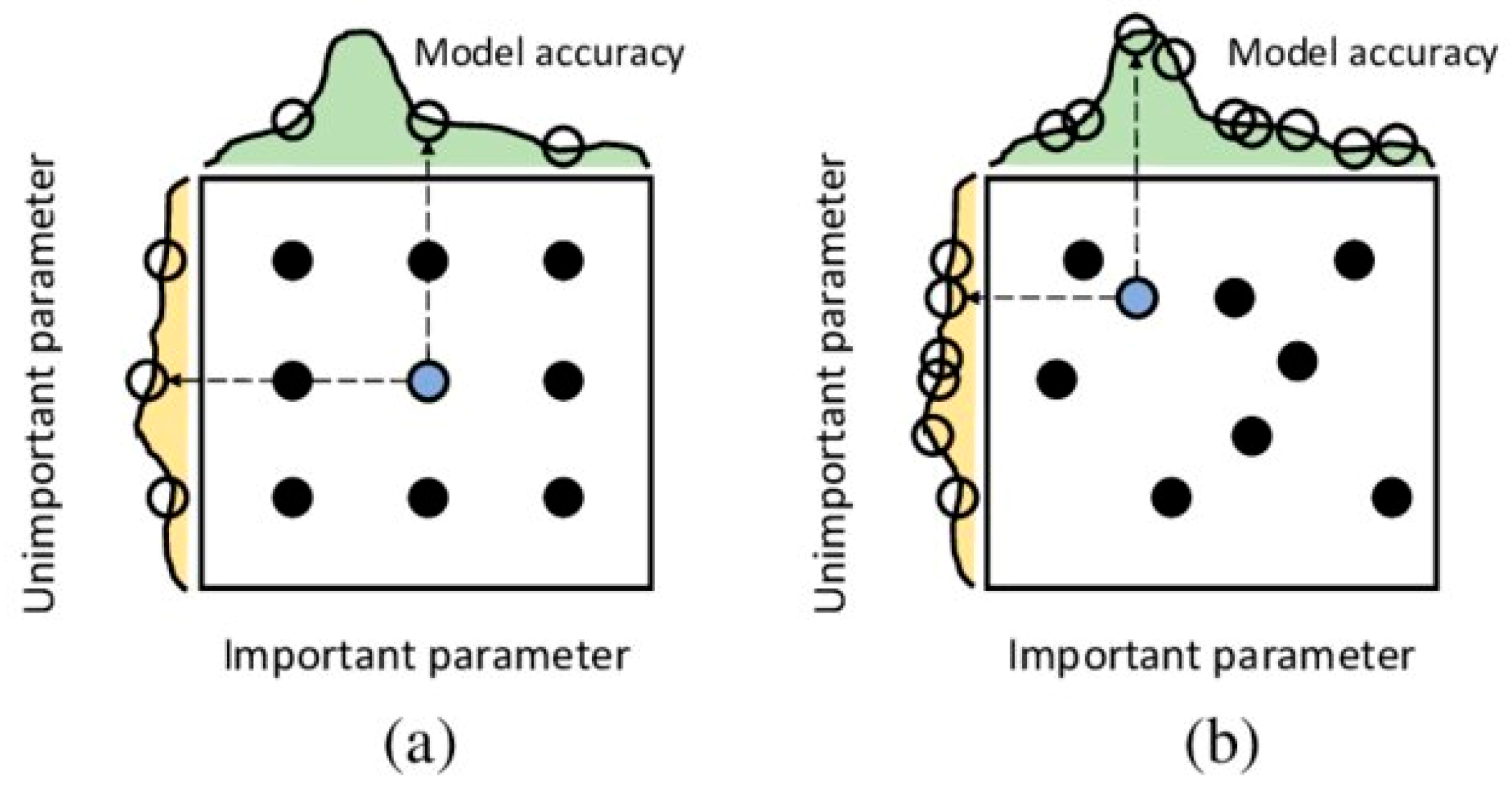
5.1. Hyperparameters Tuning Results

In this section, three ML models including GB, ANN and SVM were developed to predict the USC of the cement-stabilized soil. The hyper-parameters range of those ML models was also given in

Table 2. Hyper-parameters space of machine learning (ML) models.

Gradient Boosting		Artificial Neural Network		Support Vector Machine
Learning rate	0.01–0.3	Number of neurons	2–50	Regularization parameter (C)	0.001–1000
Number of tree	10–300	Solver (*)	1, 2, 3	Kernel coefficient Gamma (γ)	0.001–1
Min samples split	2–20	Activation function (**)	1, 2, 3	Kernel type (***)	1, 2, 3
Min samples leaf	2–20	Max iteration	1000–4000
Max depth	0–20	Learning rate	0.001–0.2
Data used	5Fold CV	Data used	5Fold CV	Data used	5Fold CV
Performance index	R	Performance index	R	Performance index	R

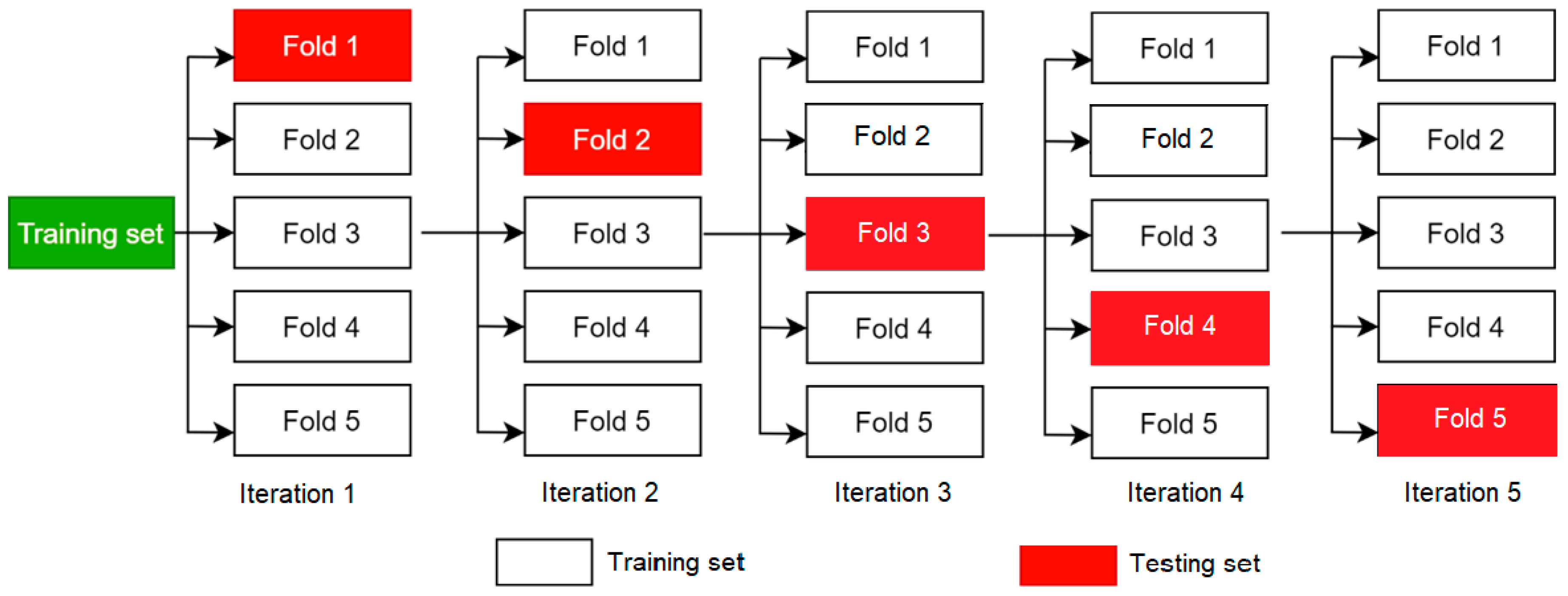
(*): 1—Quasi-Newton method; 2—Stochastic Gradient Descent; 3—Adam; (**): 1—Logistic; 2—Tanh; 3—Relu; (***): 1—Polynomial; 2—Radial basis function; 3—Sigmoid.

. To prepare the data for the hyper-parameters tuning process, the initial data set was random divided into two sets, including the training set (80%) and testing set (20%). To avoid data leakage, ML models were evaluated based on data from the 5 fold CV technique, which mean testing data was hidden in this step.

In the process of hyper-parameter tuning, the model with the best R performance indicator was selected as the final model and the model’s hyper-parameters were considered the optimum hyper-parameters. A summary of the optimal hyper-parameters of each model was presented in

Table 3. Optimum hyper-parameters of ML models.

Gradient Boosting		Artificial Neural Network		Support Vector Machine
Learning rate	0.2	Number of neurons	50	Regularization parameter (C)	1000
Number of tree	117	Solver	Adam	Kernel coefficient Gamma (γ)	0.1
Min samples split	9	Activation function	Logistic	Kernel type	Radial bias function
Min samples leaf	3	Max iteration	3000
Max depth	16	Learning rate	0.1
Best criteria R	0.929	Best criteria R	0.93	Best criteria R	0.871

.

It can be seen that all three models showed good performance after hyper-parameter optimization when the R criterion was above 0.87. The hyper-parameters combined quite complexly to create the best model. In the GB model, the higher learning rate seemed to bring better performance when in the ANN model, Adam was the best training algorithm for this data set. Furthermore, the SVM model with the kernel type of the radial basis function gives better performance than the sigmoid function. Besides, the lower the gamma on SVM model, the lower the performance. Out of the three models, ANN and GB showed outstanding performance compared to the SVM model. To be more specific, the best R criteria of the ANN and GB model was 0.93 and 9.29 respectively compared to 0.871 of the SVM model.

5.2. Comparison of GB, ANN and SVM

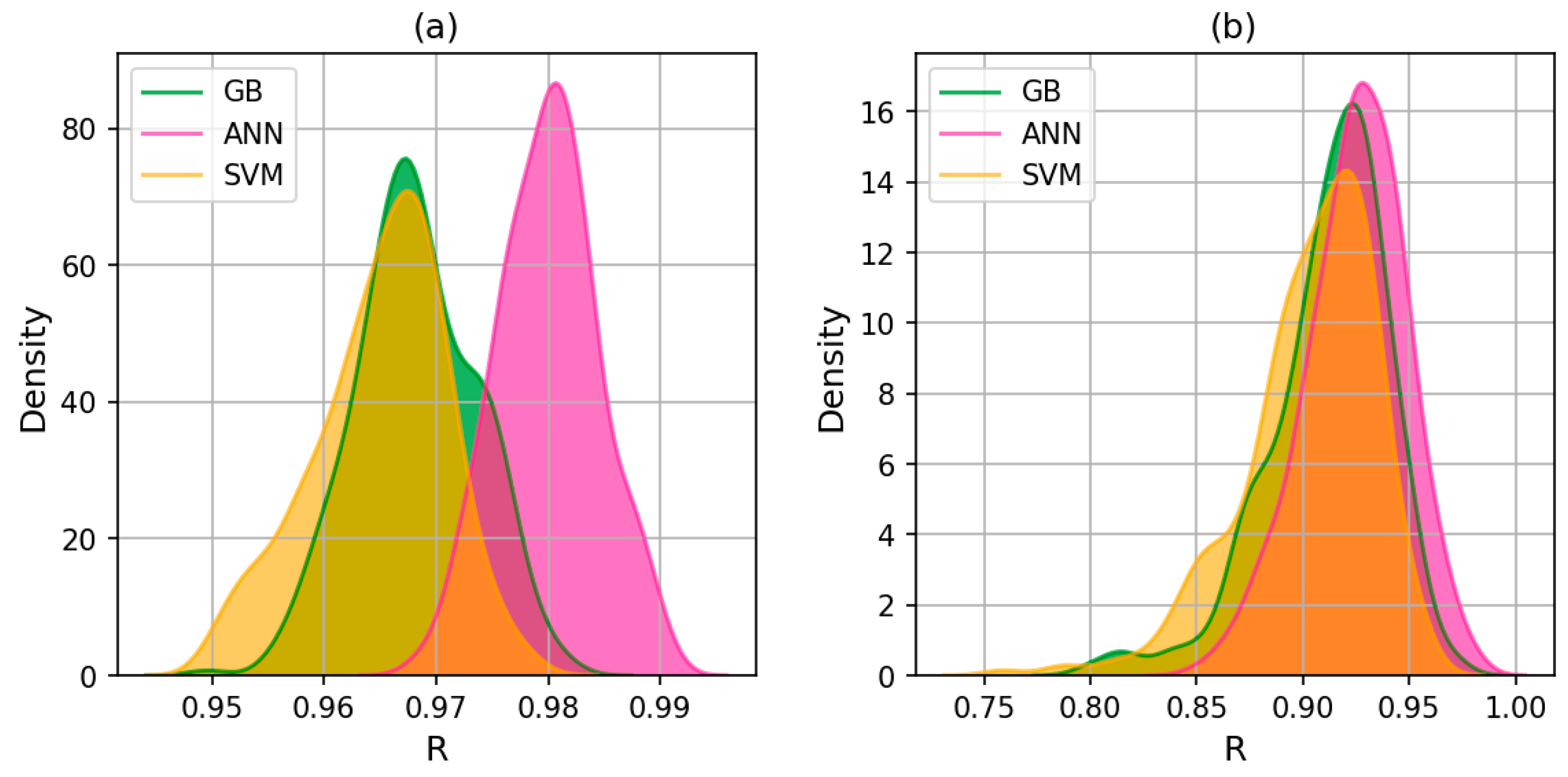
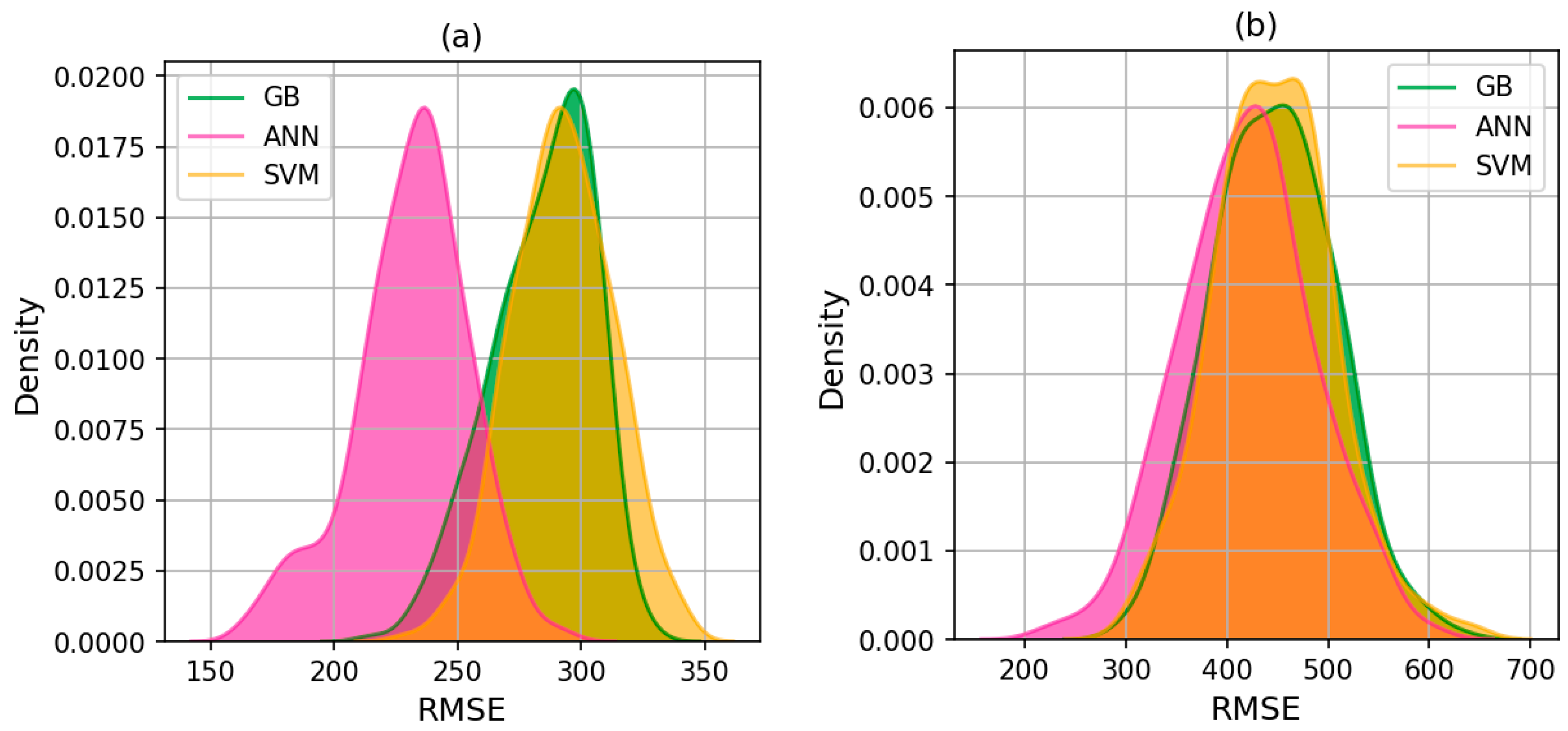
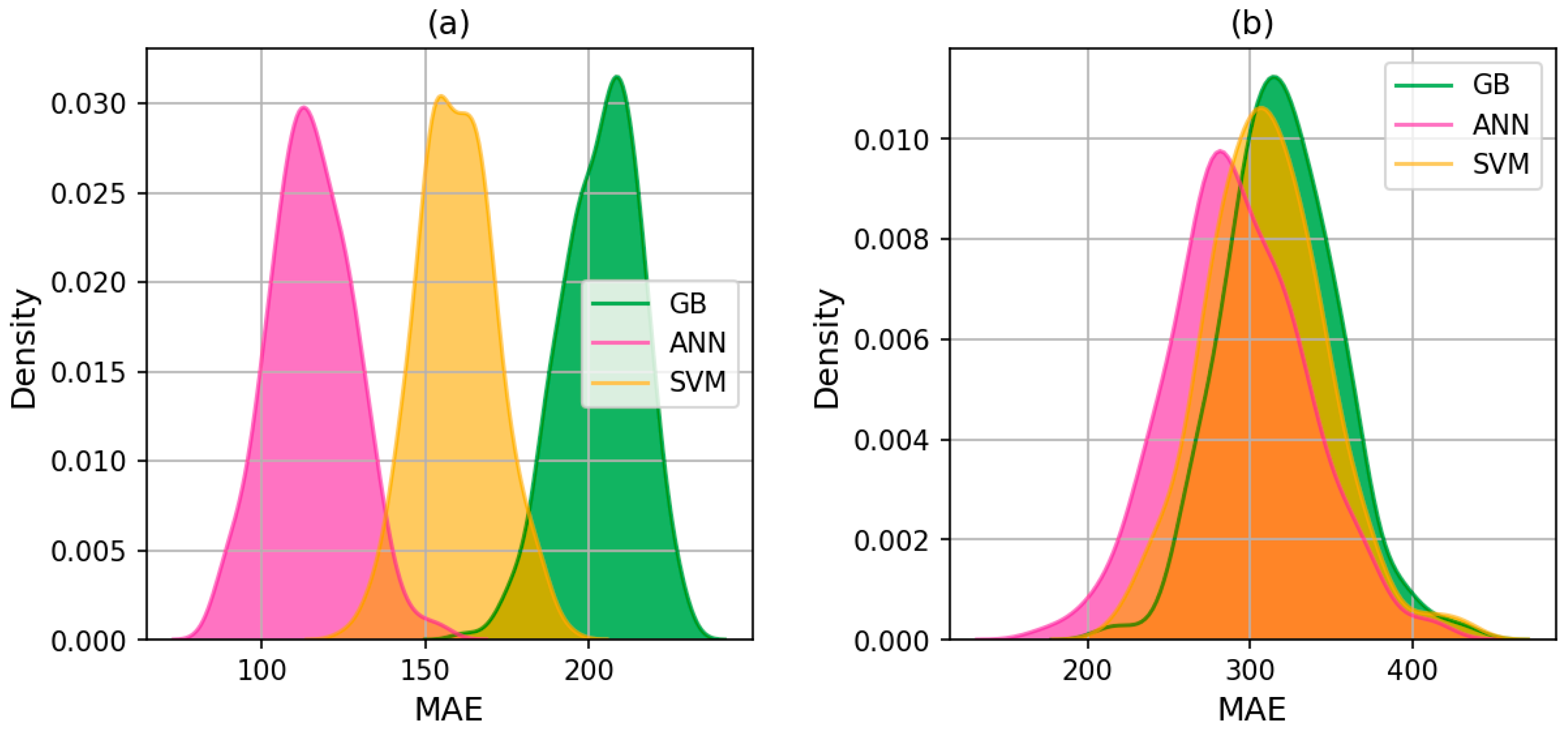
From a statistical standpoint, the randomness in the data set needed to be carefully considered when comparing models. In this section, to compare the performance of the three optimized models, 300 samplings were performed taking into account the random division between training set and testing set. In these samplings, the training and test set sizes were kept the same, however the index number of the training and test data were randomly selected in the original data set. The models would be built on the training set and then validated on the testing set.

Figure 8, Figure 9 and Figure 10 showed a density curve of the performance results after 300 samplings on the training set and testing set. The summary of the performance indicators of each models was presented in

Table 4. Summary of the 300 samplings using R criteria.

Model	Dataset	Average	Min	Max	SD (*)
GB	Training	0.968	0.968	0.982	0.005
	Testing	0.912	0.798	0.973	0.029
ANN	Training	0.980	0.968	0.991	0.004
	Testing	0.925	0.850	0.981	0.031
SVM	Training	0.965	0.950	0.979	0.006
	Testing	0.903	0.759	0.957	0.031

SD ⁽*⁾ = Standard Deviation.

,

Table 5. Summary of the 300 samplings using RMSE criteria.

Model	Dataset	Average	Min	Max	SD (*)
GB	Training	284.41	215.58	327.34	20.23
	Testing	446.79	298.94	629.76	58.71
ANN	Training	231.2	163.03	292.94	23.16
	Testing	419.82	221.04	599.35	65.91
SVM	Training	292.7	229.11	341.08	19.97
	Testing	446.67	299.93	641.16	58.59

SD ⁽*⁾ = Standard Deviation.

and

Table 6. Summary of the 300 samplings using MAE criteria.

Model	Dataset	Average	Min	Max	SD (*)
GB	Training	203.49	161.85	229.3	11.92
	Testing	319.23	211.68	436.57	34.91
ANN	Training	115.29	86.01	155.6	12.71
	Testing	292.2	171.95	413.51	41.57
SVM	Training	159.5	125.69	193.39	11.87
	Testing	309.76	215.35	434.12	37.3

SD ⁽*⁾ = Standard Deviation.

. It can be seen that the values of R of all three models showed a strong prediction UCS of cement-stabilized soil as the values of R were in the range of 0.9–1 on the training set and in the range of 0.8–1 on the testing set. The values of RMSE were in the range of 150–350 (kPa) on training set and in the range of 200–650 (kPa) on the testing set while the value of MAE varied from 50 to 250 (kPa) on the training set and from 100 to 400 (kPa) on the testing set.

It also can be seen that out of the three models, the ANN model gave outstanding performance, reflected in the average of all performance indicators, namely R = 0.925, RMSE = 419.82 and MAE = 292.2 on testing set. The GB and SVM models showed equal performance when the GB model had better performance at R but worse at RMSE and MAE. To be more specific, GB had the average performance indicator of R = 0.912, RMSE = 446.79 and MAE =319.23 while SVM model had the average criteria R = 0.903, RMSE = 446.67 and MAE = 309.76 on the testing set. In addition, the minimum and maximum values of the performance indicators of the ANN model all allowed it to outperform the other models, proving that the model was more stable.

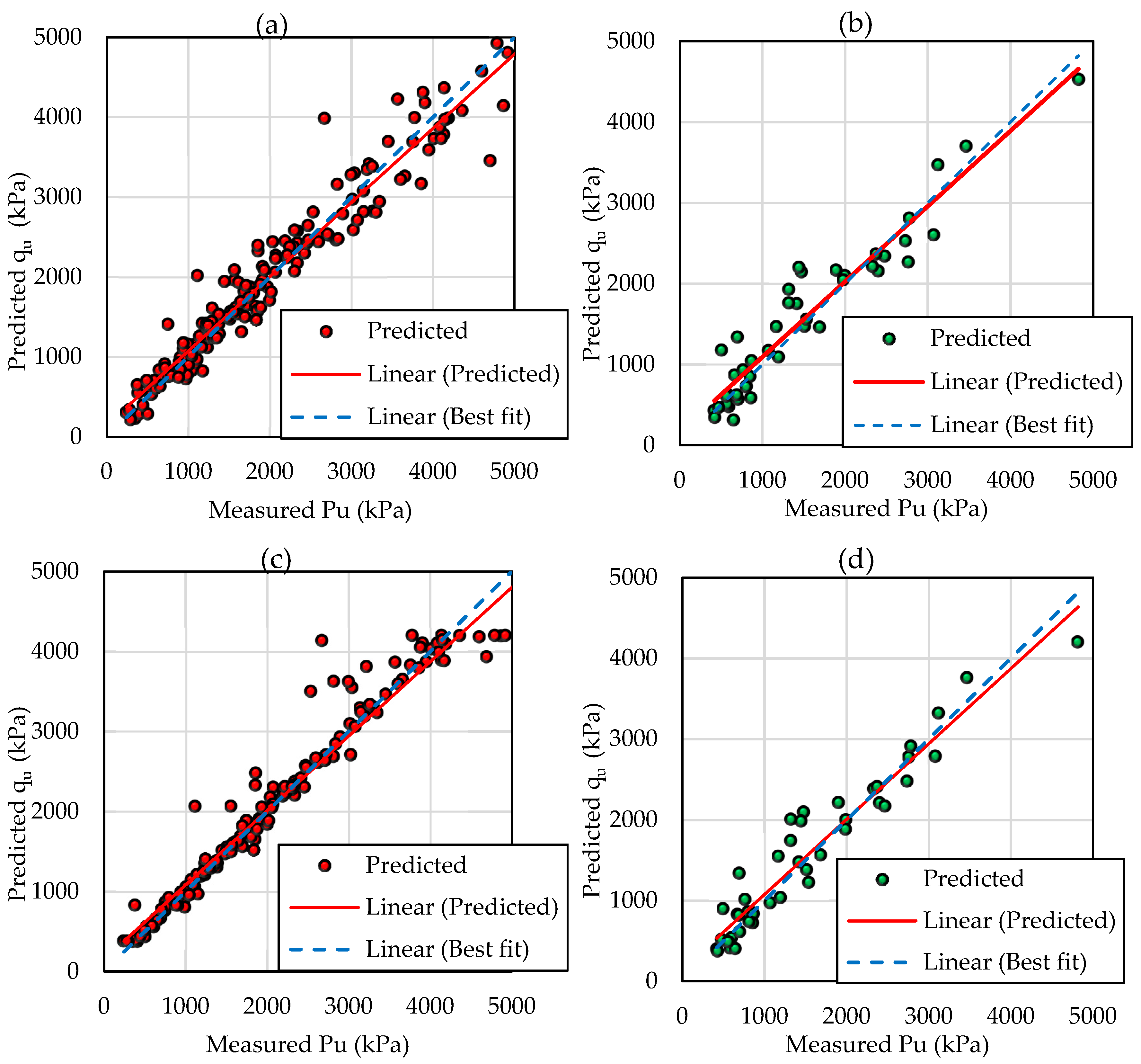
5.3. Predictability of Models

In this section, the results of typical ML models were presented. All three models showed good prediction when the linear fit almost overlapped with the best fit on both the training set and testing set (Figure 11). Out of the three models, ANN showed the best performance when all prediction points on the training and testing set were almost closest to the perfect fit. Based on the analysis results, it can be confirmed that the ML models were successful in predicting UCS of the cement-stabilized soil and optimized ANN was the most suitable model for this data set.

Table 7. Comparison with previous studies.

Author	Model	Sample Type	Number of Samples	R	RMSE
Suman et al. [18]	FN	Cement stabilized soil	58	0.95	-
	MARS			0.95	-
	MLR			0.73	-
Hoang-Anh Le et al. [21]	GPR	UCS of soil	118	0.861	0.442
Das et al. [20]	BRNN	Cement stabilized soil	55	0.87	-
	LMNN			0.851	-
	DENN			0.846	-
The present study	RS-ANN	Cement stabilized soil	216	0.925	419.82
	RS-GB			0.912	446.79
	RS-SVM			0.903	446.67

presented some previous research results on ML applications in determining USC of some soil type. The results of the present study and previous studies show the expected effect of the ML technique in determining the UCS of soils with most of the R reaching between 0.8 and 0.95 on the testing data set. However, due to the use of different data sets, the comparison among these results make no sense. A project that combines datasets from different studies is needed to create a large database for building generalized models in the UCS prediction of soil reinforcement.

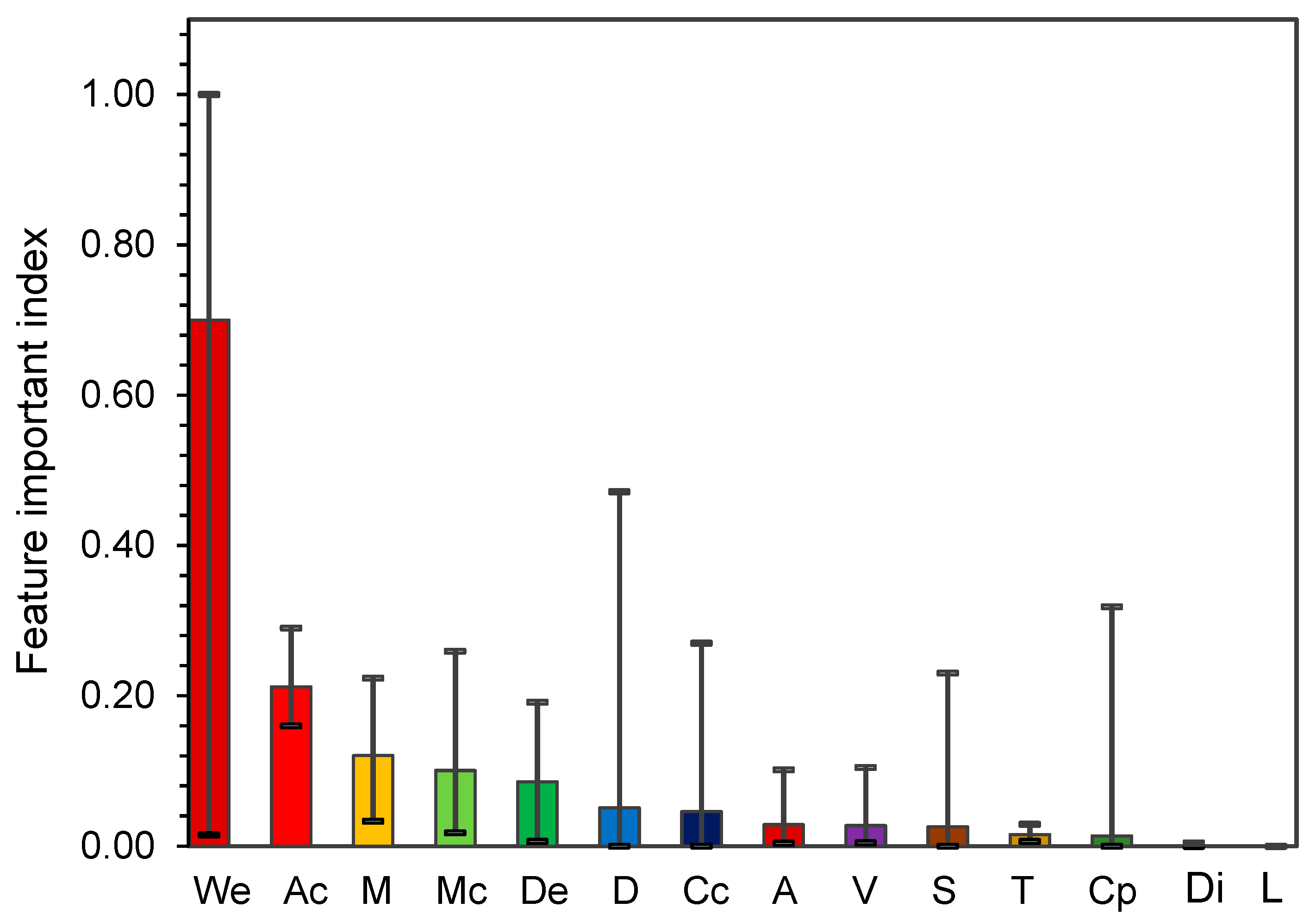
5.4. Feature Importance Analysis

The GB algorithm allows estimating the importance of input features. In fact, the GB algorithm included many decision trees and for each tree, the feature importance of an input variable was calculated as the fraction of samples that will traverse a node that splits based on that variable. The mean score of all trees then decided the important index of each features. The important index scores will be in the range [0, 1] and the higher scores the more important the feature.

The result shown on Figure 12: It can be seen that amongst the 14 input variables that used to detect the UCS of cement-stabilized soil, the wet density (We) and the amount of cement (Ac) was the most important features, which score an average sensitive index of 0.7 and 0.212, respectively. From a soil mechanic point of view, We affects the unit weight of soil or decides particle density while the amount of cement (Ac) decides the cohesion between the soil particles, so both of them play an important role in predicting the UCS of cement-stabilized soil. The variables M, Mc and De were ranked as the third to the fifth important predictors with an average sensitive index, ranging from 0.12 to 0.085. The other variables such as D, Cc, A, V and S had a lower sensitive index, ranging from 0.051 to 0.026, indicating that they are not affected much by the regression result. Remain features include T, Cp, Di and L, which had an important index lower than 0.006, showing that they nearly did not affect the prediction result.

6. Conclusions

The main aim of this study was to develop three machine-learning methods to predict the USC of cement-stabilized soil. The models were optimized by the RS technique to find out the best architecture including some hyper-parameters that had a significant effect on the performance of machine learning models.

The results showed that all three optimized machine-learning model including GB, ANN and SVR had an impressive ability in predicting the USC of cement-stabilized soil with R criteria ranging from 0.85 to 1. Besides, 300 simulations including randomization of data between the training set and the testing set were conducted. It can be seen that, among the three models used in this study, the ANN model had superior performance compared to the other two models on both training and testing training, represented in the average performance index of 300 simulations, specifically R = 0.98, RMSE = 231.2 and MAE =115.29 for the training set and R = 0.925, RMSE = 419.82 and MAE = 292.2 for the testing set.

In addition, the feature important index analysis by the GB model showed that between 14 input variables, the wet density (We) and the amount of cement (Ac) was the most important features, which play an important role in predicting of the UCS of cement-stabilized soil.

The results of this study indicated that machine learning methods, especially the ANN model, can be an effective tool for quickly predicting UCS of cement stabilized soils with excellent performance.

References

1. Bergado, D.T. Soft Ground Improvement: In Lowland and Other Environments; ASCE Press: New York, NY, USA, 1996; ISBN 0-7844-0151-9. [Google Scholar]
2. Porbaha, A. State of the Art in Deep Mixing Technology: Part I. Basic Concepts and Overview. Proc. Inst. Civ. Eng. Ground Improv. 1998, 2, 81–92. [Google Scholar] [CrossRef]
3. Chenari, R.J.; Fatahi, B.; Ghorbani, A.; Alamoti, M.N. Evaluation of Strength Properties of Cement Stabilized Sand Mixed with EPS Beads and Fly Ash. Geomech. Eng. 2018, 14, 533–544. [Google Scholar]
4. Ahmadi, H.; Bezuijen, A. Full-Scale Mechanically Stabilized Earth (MSE) Walls under Strip Footing Load. Geotext. Geomembr. 2018, 46, 297–311. [Google Scholar] [CrossRef]
5. Bergado, D.T.; Singh, N.; Sim, S.H.; Panichayatum, B.; Sampaco, C.L.; Balasubramaniam, A.S. Improvement of Soft Bangkok Clay Using Vertical Geotextile Band Drains Compared with Granular Piles. Geotext. Geomembr. 1990, 9, 203–231. [Google Scholar] [CrossRef]
6. Indraratna, B.; Rujikiatkamjorn, C.; Balasubramaniam, A.S.; McIntosh, G. Soft Ground Improvement via Vertical Drains and Vacuum Assisted Preloading. Geotext. Geomembr. 2012, 30, 16–23. [Google Scholar] [CrossRef] [Green Version]
7. Liu, S.-Y.; Du, Y.-J.; Yi, Y.-L.; Puppala, A.J. Field Investigations on Performance of T-Shaped Deep Mixed Soil Cement Column–Supported Embankments over Soft Ground. J. Geotech. Geoenviron. Eng. 2012, 138, 718–727. [Google Scholar] [CrossRef]
8. Oh, Y.I.; Shin, E.C. Reinforcement and Arching Effect of Geogrid-Reinforced and Pile-Supported Embankment on Marine Soft Ground. Mar. Georesour. Geotechnol. 2007, 25, 97–118. [Google Scholar] [CrossRef]
9. Choobbasti, A.J.; Kutanaei, S.S. Microstructure Characteristics of Cement-Stabilized Sandy Soil Using Nanosilica. J. Rock Mech. Geotech. Eng. 2017, 9, 981–988. [Google Scholar] [CrossRef]
10. Sarokolayi, L.K.; Beitollahi, A.; Abdollahzadeh, G.; Amreie, S.T.R.; Kutanaei, S.S. Modeling of Ground Motion Rotational Components for Near-Fault and Far-Fault Earthquake According to Soil Type. Arab. J. Geosci. 2015, 8, 3785–3797. [Google Scholar] [CrossRef]
11. Changizi, F.; Haddad, A. Strength Properties of Soft Clay Treated with Mixture of Nano-SiO2 and Recycled Polyester Fiber. J. Rock Mech. Geotech. Eng. 2015, 7, 367–378. [Google Scholar] [CrossRef]
12. Ghasabkolaei, N.; Janalizadeh, A.; Jahanshahi, M.; Roshan, N.; Ghasemi, S.E. Physical and Geotechnical Properties of Cement-Treated Clayey Soil Using Silica Nanoparticles: An Experimental Study. Eur. Phys. J. Plus 2016, 131, 134. [Google Scholar] [CrossRef]
13. Choobbasti, A.J.; Vafaei, A.; Kutanaei, S.S. Mechanical Properties of Sandy Soil Improved with Cement and Nanosilica. Open Eng. 2015, 5. [Google Scholar] [CrossRef] [Green Version]
14. Horpibulsuk, S.; Miura, N.; Nagaraj, T.S. Assessment of Strength Development in Cement-Admixed High Water Content Clays with Abrams’ Law as a Basis. Geotechnique 2003, 53, 439–444. [Google Scholar] [CrossRef]
15. Miura, N.; Horpibulsuk, S.; Nagaraj, T.S. Engineering Behavior of Cement Stabilized Clay at High Water Content. Soils Found. 2001, 41, 33–45. [Google Scholar] [CrossRef] [Green Version]
16. Horpibulsuk, S.; Bergado, D.T.; Lorenzo, G.A. Compressibility of Cement-Admixed Clays at High Water Content. Geotechnique 2004, 54, 151–154. [Google Scholar] [CrossRef]
17. Horpibulsuk, S.; Miura, N.; Nagaraj, T.S. Clay–Water/Cement Ratio Identity for Cement Admixed Soft Clays. J. Geotech. Geoenviron. Eng. 2005, 131, 187–192. [Google Scholar] [CrossRef]
18. Suman, S.; Mahamaya, M.; Das, S.K. Prediction of Maximum Dry Density and Unconfined Compressive Strength of Cement Stabilised Soil Using Artificial Intelligence Techniques. Int. J. Geosynth. Ground Eng. 2016, 2, 11. [Google Scholar] [CrossRef] [Green Version]
19. Narendra, B.S.; Sivapullaiah, P.V.; Suresh, S.; Omkar, S.N. Prediction of Unconfined Compressive Strength of Soft Grounds Using Computational Intelligence Techniques: A Comparative Study. Comput. Geotech. 2006, 33, 196–208. [Google Scholar] [CrossRef]
20. Das, S.K.; Samui, P.; Sabat, A.K. Application of Artificial Intelligence to Maximum Dry Density and Unconfined Compressive Strength of Cement Stabilized Soil. Geotech. Geol. Eng. 2011, 29, 329–342. [Google Scholar] [CrossRef]
21. Le, H.-A.; Nguyen, T.-A.; Nguyen, D.-D.; Prakash, I. Prediction of Soil Unconfined Compressive Strength Using Artificial Neural Network Model. Vietnam J. Earth Sci. 2020, 42, 255–264. [Google Scholar] [CrossRef]
22. Bui Truong, S.; Nguyen Thi, N.; Nguyen Thanh, D. An Experimental Study on Unconfined Compressive Strength of Soft Soil-Cement Mixtures with or without GGBFS in the Coastal Area of Vietnam. Adv. Civ. Eng. 2020, 2020, 1–12. [Google Scholar] [CrossRef]
23. Ribeiro, D.; Néri, R.; Cardoso, R. Influence of Water Content in the UCS of Soil-Cement Mixtures for Different Cement Dosages. Procedia Eng. 2016, 143, 59–66. [Google Scholar] [CrossRef] [Green Version]
24. Malizia, J.P.; Shakoor, A. Effect of Water Content and Density on Strength and Deformation Behavior of Clay Soils. Eng. Geol. 2018, 244, 125–131. [Google Scholar] [CrossRef] [Green Version]
25. Li, B. Study on the Strength Influence of Pile Driving Disturbance on the Surrounding Soil. E3S Web Conf. 2019, 136, 04078. [Google Scholar] [CrossRef]
26. Haralambos, S.I. Compressive Strength of Soil Improved with Cement. In Proceedings of the Contemporary Topics in Ground Modification, Problem Soils, and Geo-Support, American Society of Civil Engineers, Orlando, FL, USA, 10 March 2009; pp. 289–296. [Google Scholar]
27. Lan, G.; Wang, Y.; Chao, S. Influences of Specimen Geometry and Loading Rate on Compressive Strength of Unstabilized Compacted Earth Block. Adv. Mater. Sci. Eng. 2018, 2018, 1–10. [Google Scholar] [CrossRef] [Green Version]
28. Güneyli, H.; Rüşen, T. Effect of Length-to-Diameter Ratio on the Unconfined Compressive Strength of Cohesive Soil Specimens. Bull. Eng. Geol. Environ. 2015, 75. [Google Scholar] [CrossRef]
29. Friedman, J.H. Greedy Function Approximation: A Gradient Boosting Machine. Ann. Stat. 2001, 29, 1189–1232. [Google Scholar] [CrossRef]
30. Wei, L.; Yuan, Z.; Zhong, Y.; Yang, L.; Hu, X.; Zhang, Y. An Improved Gradient Boosting Regression Tree Estimation Model for Soil Heavy Metal (Arsenic) Pollution Monitoring Using Hyperspectral Remote Sensing. Appl. Sci. 2019, 9, 1943. [Google Scholar] [CrossRef] [Green Version]
31. Chopra, T.; Vajpai, J. Fault Diagnosis in Benchmark Process Control System Using Stochastic Gradient Boosted Decision Trees. Int. J. Soft Comput. Eng 2011, 1, 98–101. [Google Scholar]
32. Tziachris, P.; Aschonitis, V.; Chatzistathis, T.; Papadopoulou, M. Assessment of Spatial Hybrid Methods for Predicting Soil Organic Matter Using DEM Derivatives and Soil Parameters. Catena 2019, 174, 206–216. [Google Scholar] [CrossRef]
33. Devos, L.; Meert, W.; Davis, J. Fast Gradient Boosting Decision Trees with Bit-Level Data Structures. In Lecture Notes in Computer Science, Proceedings of the Machine Learning and Knowledge Discovery in Databases, Würzburg, Germany, 16–20 September 2019; Brefeld, U., Fromont, E., Hotho, A., Knobbe, A., Maathuis, M., Robardet, C., Eds.; Springer International Publishing: Cham, Switzerland, 2019; Volume 11906, pp. 590–606. ISBN 978-3-030-46149-2. [Google Scholar]
34. Liu, L.; Ji, M.; Buchroithner, M. Combining Partial Least Squares and the Gradient-Boosting Method for Soil Property Retrieval Using Visible near-Infrared Shortwave Infrared Spectra. Remote Sens. 2017, 9, 1299. [Google Scholar] [CrossRef] [Green Version]
35. Shahin, M.A.; Jaksa, M.B.; Maier, H.R. Artificial Neural Network Applications in Geotechnical Engineering. Aust. Geomech. 2001, 36, 49–62. [Google Scholar]
36. Subaşı, S. Prediction of Mechanical Properties of Cement Containing Class C Fly Ash by Using Artificial Neural Network and Regression Technique. Sci. Res. Essays 2009, 4, 289–297. [Google Scholar]
37. Naghibi, S.A.; Pourghasemi, H.R.; Dixon, B. GIS-Based Groundwater Potential Mapping Using Boosted Regression Tree, Classification and Regression Tree, and Random Forest Machine Learning Models in Iran. Environ. Monit. Assess. 2016, 188, 1–27. [Google Scholar] [CrossRef] [PubMed]
38. Were, K.; Bui, D.T.; Dick, Ø.B.; Singh, B.R. A Comparative Assessment of Support Vector Regression, Artificial Neural Networks, and Random Forests for Predicting and Mapping Soil Organic Carbon Stocks across an Afromontane Landscape. Ecol. Indic. 2015, 52, 394–403. [Google Scholar] [CrossRef]
39. Hecht-Nielsen, R. Theory of the Backpropagation Neural Network. In Proceedings of the International 1989 Joint Conference on Neural Networks, Washington, DC, USA, 18–21 June 1989; IEEE Press: New York, NY, USA, 1989; Volume 1, pp. 593–605. [Google Scholar]
40. Ripley, B.D.; Ripley, R.M. Neural networks as statistical methods in survival analysis. In Clinical Applications of Artificial Neural Networks; Dybowski, R., Gant, V., Eds.; Cambridge University Press: Cambridge, UK, 2001; pp. 237–255. ISBN 978-0-521-66271-0. [Google Scholar]
41. Zhao, Z.; Chow, T.L.; Rees, H.W.; Yang, Q.; Xing, Z.; Meng, F.-R. Predict Soil Texture Distributions Using an Artificial Neural Network Model. Comput. Electron. Agric. 2009, 65, 36–48. [Google Scholar] [CrossRef]
42. Chou, J.-S.; Yang, K.-H.; Lin, J.-Y. Peak Shear Strength of Discrete Fiber-Reinforced Soils Computed by Machine Learning and Metaensemble Methods. J. Comput. Civ. Eng. 2016, 30, 04016036. [Google Scholar] [CrossRef] [Green Version]
43. Lu, J.; Yu, Z.; Zhu, Y.; Huang, S.; Luo, Q.; Zhang, S. Effect of Lithium-Slag in the Performance of Slag Cement Mortar Based on Least-Squares Support Vector Machine Prediction. Materials 2019, 12, 1652. [Google Scholar] [CrossRef] [Green Version]
44. Wu, J.; Chen, X.-Y.; Zhang, H.; Xiong, L.-D.; Lei, H.; Deng, S.-H. Hyperparameter Optimization for Machine Learning Models Based on Bayesian Optimizationb. J. Electron. Sci. Technol. 2019, 17, 26–40. [Google Scholar] [CrossRef]
45. Liashchynskyi, P.; Liashchynskyi, P. Grid Search, Random Search, Genetic Algorithm: A Big Comparison for NAS. arXiv 2019, arXiv:1912.06059. [Google Scholar]
46. Bergstra, J.; Bengio, Y. Random Search for Hyper-Parameter Optimization. J. Mach. Learn. Res. 2012, 13, 281–305. [Google Scholar]
47. Pham, T.A.; Tran, V.Q.; Vu, H.-L.T.; Ly, H.-B. Design Deep Neural Network Architecture Using a Genetic Algorithm for Estimation of Pile Bearing Capacity. PLoS ONE 2020, 15, e0243030. [Google Scholar] [CrossRef] [PubMed]
48. Pham, B.T.; Qi, C.; Ho, L.S.; Nguyen-Thoi, T.; Al-Ansari, N.; Nguyen, M.D.; Nguyen, H.D.; Ly, H.-B.; Le, H.V.; Prakash, I. A Novel Hybrid Soft Computing Model Using Random Forest and Particle Swarm Optimization for Estimation of Undrained Shear Strength of Soil. Sustainability 2020, 12, 2218. [Google Scholar] [CrossRef] [Green Version]
49. Shekar, B.H.; Dagnew, G. Grid Search-Based Hyperparameter Tuning and Classification of Microarray Cancer Data. In Proceedings of the 2019 Second International Conference on Advanced Computational and Communication Paradigms (ICACCP), Gangtok, India, 25–28 February 2019; pp. 1–8. [Google Scholar]
50. Schober, P.; Boer, C.; Schwarte, L.A. Correlation Coefficients: Appropriate Use and Interpretation. Anesth. Analg. 2018, 126, 1763–1768. [Google Scholar] [CrossRef]
51. Chai, T.; Draxler, R.R. Root Mean Square Error (RMSE) or Mean Absolute Error (MAE)? GMDD 2014, 7, 1525–1534. [Google Scholar]
52. Fortin, V.; Abaza, M.; Anctil, F.; Turcotte, R. Why Should Ensemble Spread Match the RMSE of the Ensemble Mean? J. Hydrometeorol. 2014, 15, 1708–1713. [Google Scholar] [CrossRef]
Figure 1. Experiment location.
Applsci 11 01949 g001
Figure 2. Undisturbed samples.
Applsci 11 01949 g002
Figure 3. Unconfined compression test equipment.
Applsci 11 01949 g003
Figure 4. Axial stress–strain relation.
Applsci 11 01949 g004
Figure 5. Diagram of a fully connected artificial neural network (ANN) with one hidden layer and a single output value.
Applsci 11 01949 g005
Figure 6. Comparison between (a) grid search and (b) random search for hyper-parameter tuning [50].
Applsci 11 01949 g006
Figure 7. Flow chart of the 5-fold cross-validation technique.
Applsci 11 01949 g007
Figure 8. Density curve of the performance indicator R on 300 samplings with the: (a) Training set and (b) Testing set.
Applsci 11 01949 g008
Figure 9. Density curve of the performance indicator RMSE on 300 samplings with the: (a) Training set and (b) Testing set.
Applsci 11 01949 g009
Figure 10. Density curve of the performance indicator MAE on 300 samplings with the: (a) Training set and (b) Testing set.
Applsci 11 01949 g010
Figure 11. Measure and predicted values of unconfined compressive strength (UCS) of cement-stabilized soil using the training set: (a) gradient boosting (GB); (c) ANN and (e) support vector machine (SVM) and testing set: (b) GB; (d) ANN and (f) SVM.
Applsci 11 01949 g011aApplsci 11 01949 g011b
Figure 12. Feature importance index of 14 variables used in this study.
Applsci 11 01949 g012