Design and Validation of an Adjustable Large-Scale Solar Simulator


Department of Industrial Engineering and Mathematical Sciences, Università Politecnica delle Marche, Via Brecce Bianche 1, 60131 Ancona, Italy
*
Author to whom correspondence should be addressed.
Appl. Sci. 2021, 11(4), 1964; https://0-doi-org.brum.beds.ac.uk/10.3390/app11041964
Submission received: 2 February 2021
/
Revised: 15 February 2021
/
Accepted: 18 February 2021
/
Published: 23 February 2021
(This article belongs to the Section Energy Science and Technology)
Abstract
:This work presents an adjustable large-scale solar simulator based on metal halide lamps. The design procedure is described with regards to the construction and spatial arrangement of the lamps and the designed optical system. Rotation and translation of the lamp array allow setting the direction and the intensity of the luminous flux on the horizontal plane. To validate the built model, irradiance nonuniformity and temporal instability tests were carried out assigning Class A, B, or C for each test, according to the International Electrotechnical Commission (IEC) standards requirements. The simulator meets the Class C standards on a 200 × 90 cm test plane, Class B on 170 × 80 cm, and Class A on 80 × 40 cm. The temporal instability returns Class A results for all the measured points. Lastly, a PV panel is characterized by tracing the I–V curve under simulated radiation, under outdoor natural sunlight, and with a numerical method. The results show a good approximation.
1. Introduction
The transient nature of environmental parameters, especially solar radiation, makes outdoor technology testing uncontrollable. Solar simulators are devices that provide approximately natural sunshine with an artificial light source and allow controllable indoor testing under desirable conditions. In fact, solar radiation, in a natural environment, changes continuously over days and seasons, while indoor tests are programmable, repeatable, and stable under laboratory conditions. This way it is possible to change a single parameter (for example, the intensity or the incidence angle of the luminous flux) and to analyze how the system is affected by each of them. Crucial aspects of the design of a solar simulator are the correct spectral matching, irradiance uniformity, and temporal stability. When testing PV cells, the spectrum is paramount since it influences the conversion efficiency of the incident radiation. Flux uniformity and stability have to be acceptable so that the average value is as stable as possible on the target area. Early solar simulators were designed in the 1960s by the National Aeronautics and Space Administration (NASA) for spacecraft ground-testing. Recently, solar simulators have been used in testing, calibrating, and characterizing photovoltaic panels and testing dashboards, steering wheels, and airbags in the automotive industry. Indeed, they have been used in many different applications, such as conducting aging tests on PV materials, investigating the effects of light on the growth of plants and algae, and testing of thermal or thermo-chemical devices for use in chemical reforming.
In thermal applications, solar simulators are classified as low and high flux, depending on the output flux, for a few suns (1 sun = 1 kW/m2) to more than 30 suns, respectively.
The major components of a solar simulator are the light source with power supply and the optics and filters to modify the output beam. Light-source selection is the primary step to obtain suitable simulated radiation. Generally, four types of lamps are used in a solar simulator: xenon arc lamps, metal halide arc lamps, light-emitting diodes (LEDs), and quartz tungsten halogen lamps. In the literature, examples can be found of solar simulators employing tungsten halogen [1,2], argon arc [3], metal halide [4,5], xenon arc [6,7], and LED lamps [8,9] or several light sources [10,11].
Many differences are present even regarding the number of lamps and target area. Moss et al. [1] designed and built a solar simulator for testing flat-plate thermal collectors (0.5 × 0.5 m). They utilized a small number of lamps and a reflected light tube that generates multiple virtual images. This way, the standard deviation in illumination over the collector area is 5.3% of the mean level. Meng et al. [5], instead, designed and built a large-scale solar simulator based on 188 lamps. The simulated radiation can be adjusted between 150 and 1100 W/m2 by varying the number of lamps on and the lamp-to-area distance. At the height of 1.75 m, the nonuniformity of illumination is 4.91%. Kolberg et al. [8] used a combination of different light sources to cover the solar spectrum. Red, green, and blue light-emitting diodes (LEDs) matched the visible range, and then UV and near-infrared lamps completed the spectrum. Watjanatepin [10] used 9 warm-white LED lamps, 9 cool-white LED lamps, 20 UV LED (410 nm) lamps, 20 IR-LED (700–800 nm) lamps, 20 IR-LED (800–900 nm) lamps, and 20 IR-LED (900–1100 nm) lamps. The calculation results of nonuniformity on the test area of 32.5 cm × 28 cm is equal to 1.915%, showing a high uniformity because of the LEDs’ symmetrical position. Leary et al. [12] compared LED and xenon lamps by measuring the current–voltage (IV) response and spectral response (SR) for a variety of solar cells. The results demonstrate that the LED-based simulator produced a more stable, flexible, and accurate match to AM1.5G than the xenon lamp-based simulator. Esen et al. [13], with 24 power LEDs and six different wavelengths, obtained a difference under 2% regarding the spectral match compared to natural sunshine. Sabahi et al. [14] performed theoretical simulations before designing the real model. This is very helpful for investigating the best arrangement of lamps to obtain a proper uniformity.
Light sources differ in lifetime, cost, collimation, flux magnitude, and color temperature. The color temperature is an important parameter because it indicates the equivalent blackbody radiator temperature and influences the spectral quality. The reference solar spectrum is provided by the ASTM G173-03 standard [15] at optical air mass AM 1.5. The maximum acceptable deviation over the test area is 15% (ISO 9806) [16]. The sun can be considered as a blackbody radiator at a temperature of approximately 5800 K [17]. A light source with a lower temperature will have a higher energy content in the infrared spectrum and a lower contribution in the visible spectrum (as occurs in tungsten halogen lamps with a color temperature of about 2100–3350 K). Instead, with high color temperatures, the opposite result will be obtained (argon lamps have a color temperature of about 6500 K and a higher energy content in the visible light range).
A series of standards [16,18,19,20] defines some parameters which a solar simulator needs to meet, regarding spectral quality, collimation, flux magnitude, and range of obtainable flux. The collimation condition of the simulated solar radiation is satisfied if at least 80% of the irradiance received at any point on the test area has emanated from a region of the solar simulator contained within a subtended angle of 60° or less. For the flux magnitude, more than 700 W/m2 is required on the test area, while the permitted deviation should be in the range of ±50 W/m2.
This paper presents the design and the validation of an adjustable solar simulator based on 20 metal halide lamps and a parabolic optical system. Nonuniformity and temporal instability tests are investigated in accordance with the IEC 60904-9 standard [21]. Further validation is proposed by characterizing the I–V curve of a PV panel, comparing the results obtained from indoor and outdoor measurements and through a software-implemented numerical model. This paper is organized as follows: in Section 2, the designed solar simulator is presented, regarding the construction, the light source selection, and the optic system utilized; in Section 3, the series of tests is listed with the results obtained; and in Section 4, the conclusions are summarized.
2. Materials and Methods
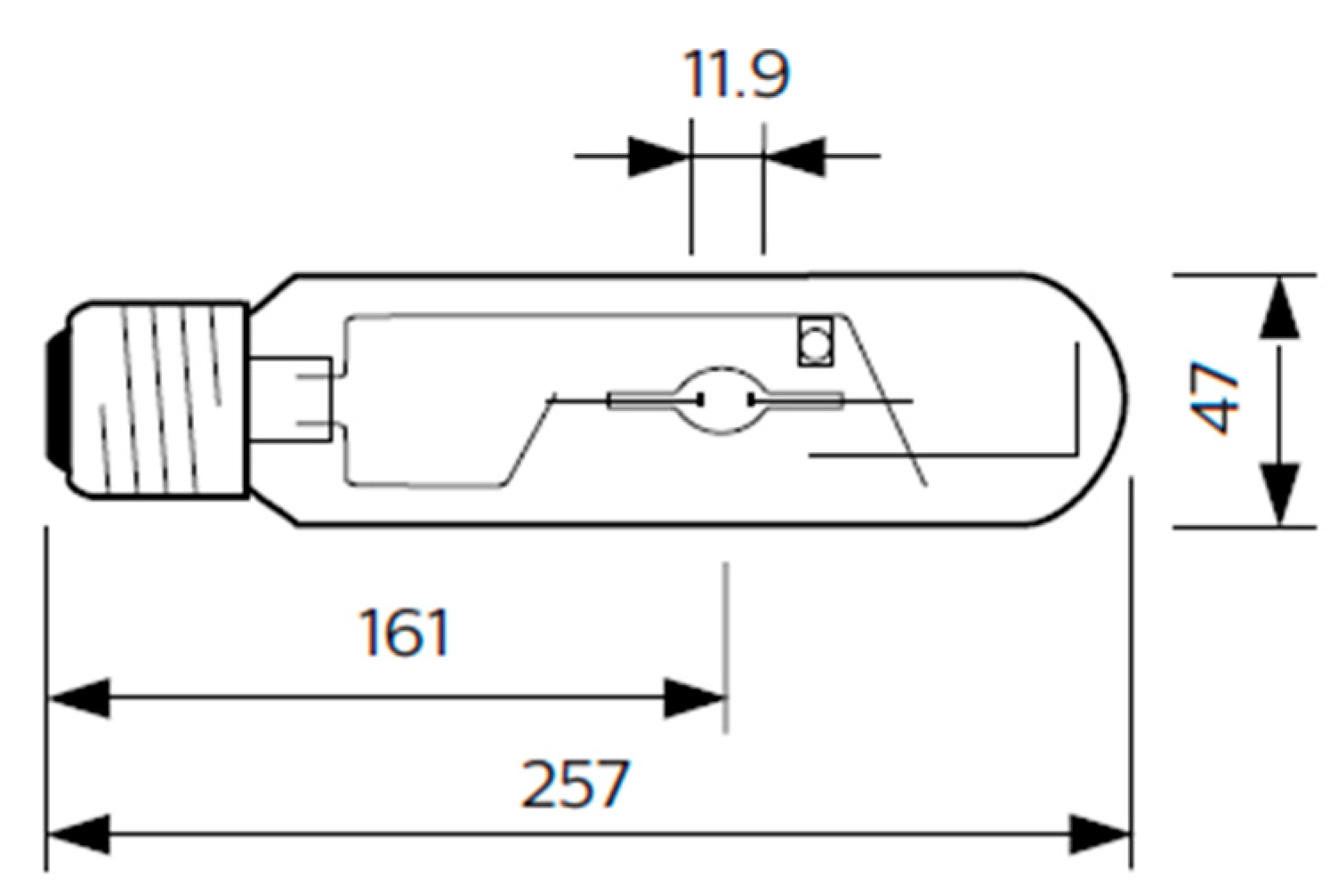
The proposed solar simulator is based on metal halide lamps, model Philips MASTER Colour CDM-T MW eco/360 W842 E40 [22] (Figure 1). It is a lamp in ceramic with clear tubular external bulb. In metal halide lamps, the electric arc is generated through a gaseous mixture of vaporized mercury and metal halide compounds held at a pressure between 10 and 35 bar [23]. They have been chosen for their long lifetime (99% after 6000 h and 90% after 16,000 h) and their relatively low cost. Each has a power of 360 W, powered with 3.6 A and 124 V, and a color temperature of 4200 K. The total power is around 7.2 kW.
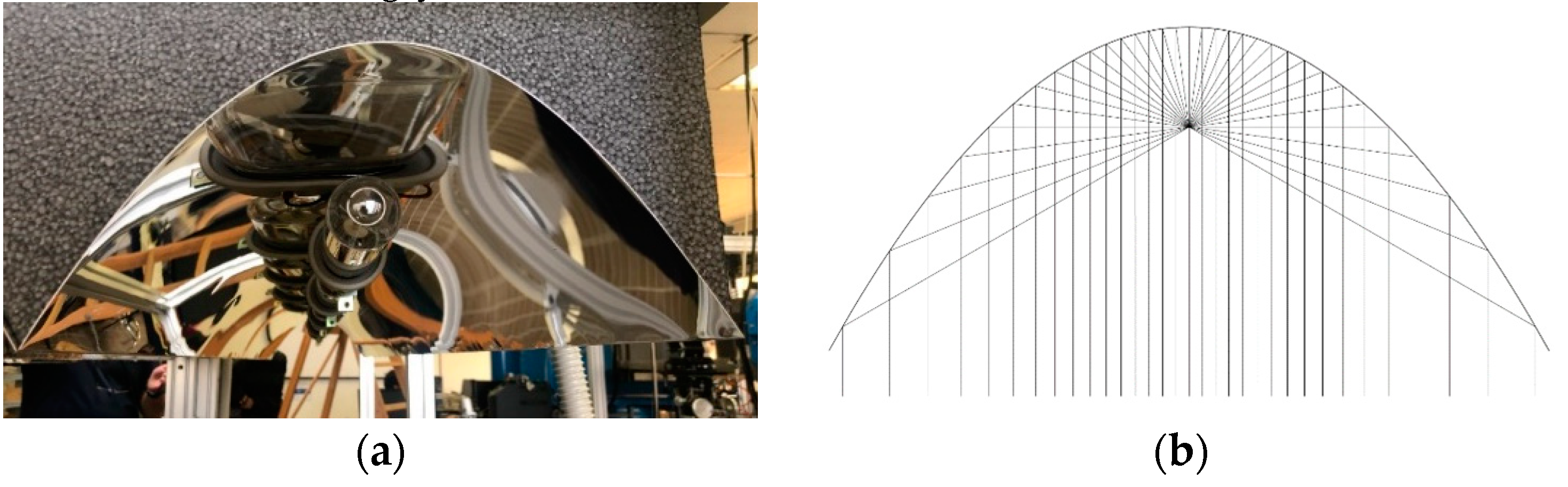
The lamps are mounted on the focal point of parabolic mirrors to create a luminous flux of uniform intensity on the target surface (Figure 2a). In fact, rays coming from the focus, after being reflected, move parallel to the optical axis, regardless of the distance of the surface. The theoretical path of the incident rays on a parabola is represented in Figure 2b, provided that the surface is perfectly smooth and follows the correct equation. The reflective material used is a thin sheet of aluminum, with an average reflection coefficient of 0.99 in the spectral range. Given the equation of a parabola,
the focal distance F is located at
where
y = ax2 + bx + c,
In this work, parameters a, b, and c are set to the values of 6, 0, and 0, respectively. Accordingly, the focal distance is located at 4.1 cm from the mirror axis.
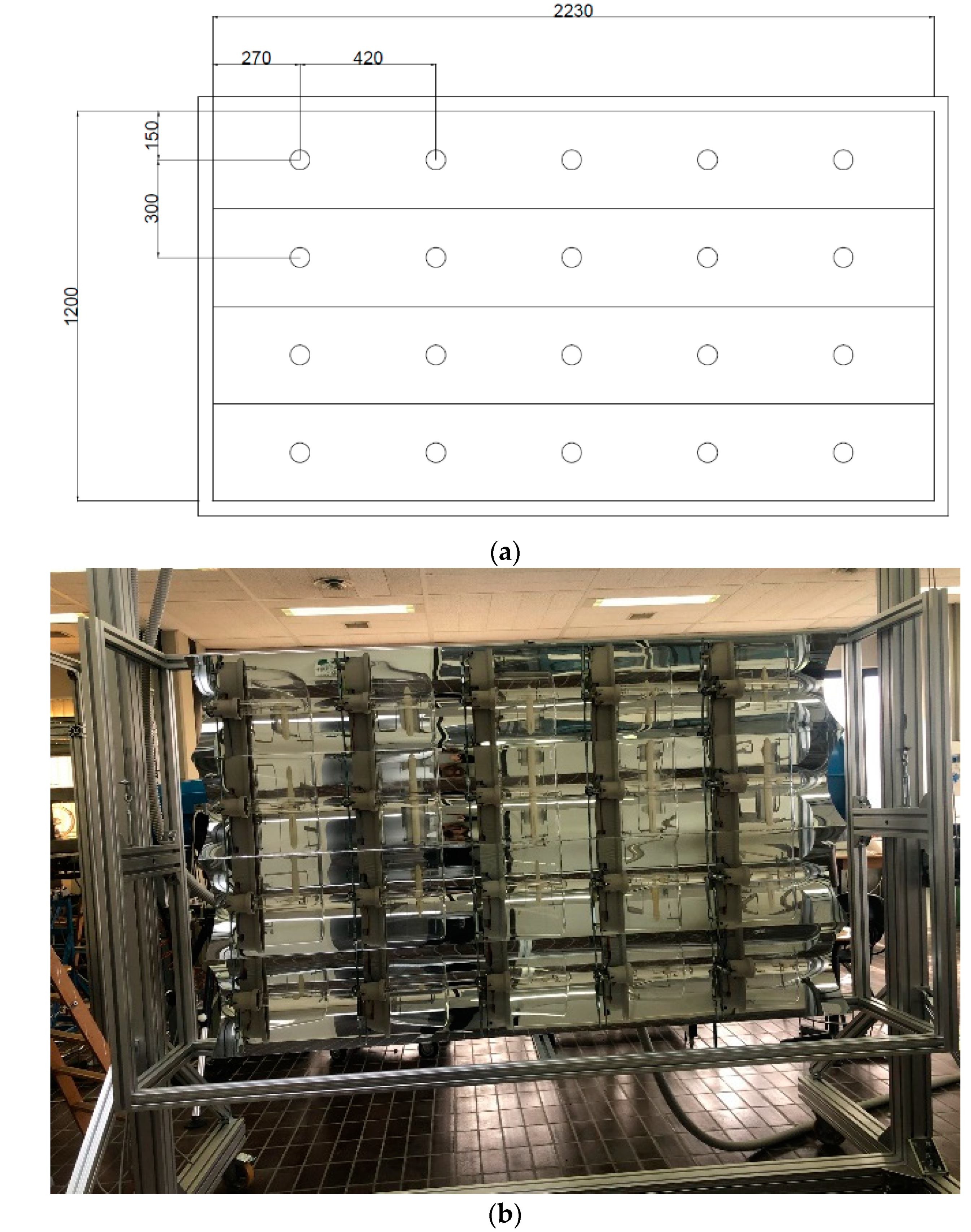
The proposed solar simulator is a multilamp pattern with 20 lamps arranged in four rows of five lamps each (Figure 3). This creates a large target surface with the same luminous characteristics.
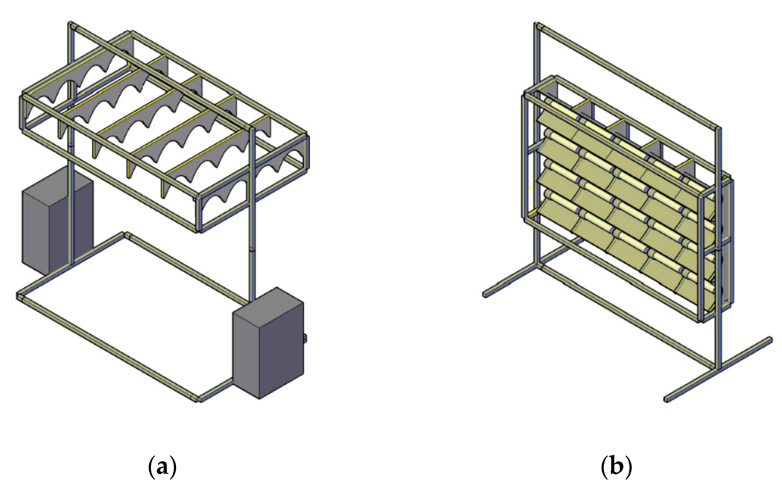
The lamp system is mounted on a structure made of aluminum profiles. The parabolas were glued on specially shaped wooden boards and mounted on the aluminum structure (Figure 4a). The system is equipped with a vertical guide to adjust the lamp–target distance and vary the intensity of the simulated radiation. It can also rotate to simulate an incident radiation not perpendicular to the plane (Figure 4b). Figure 4 depicts the 3D CAD reproduction.
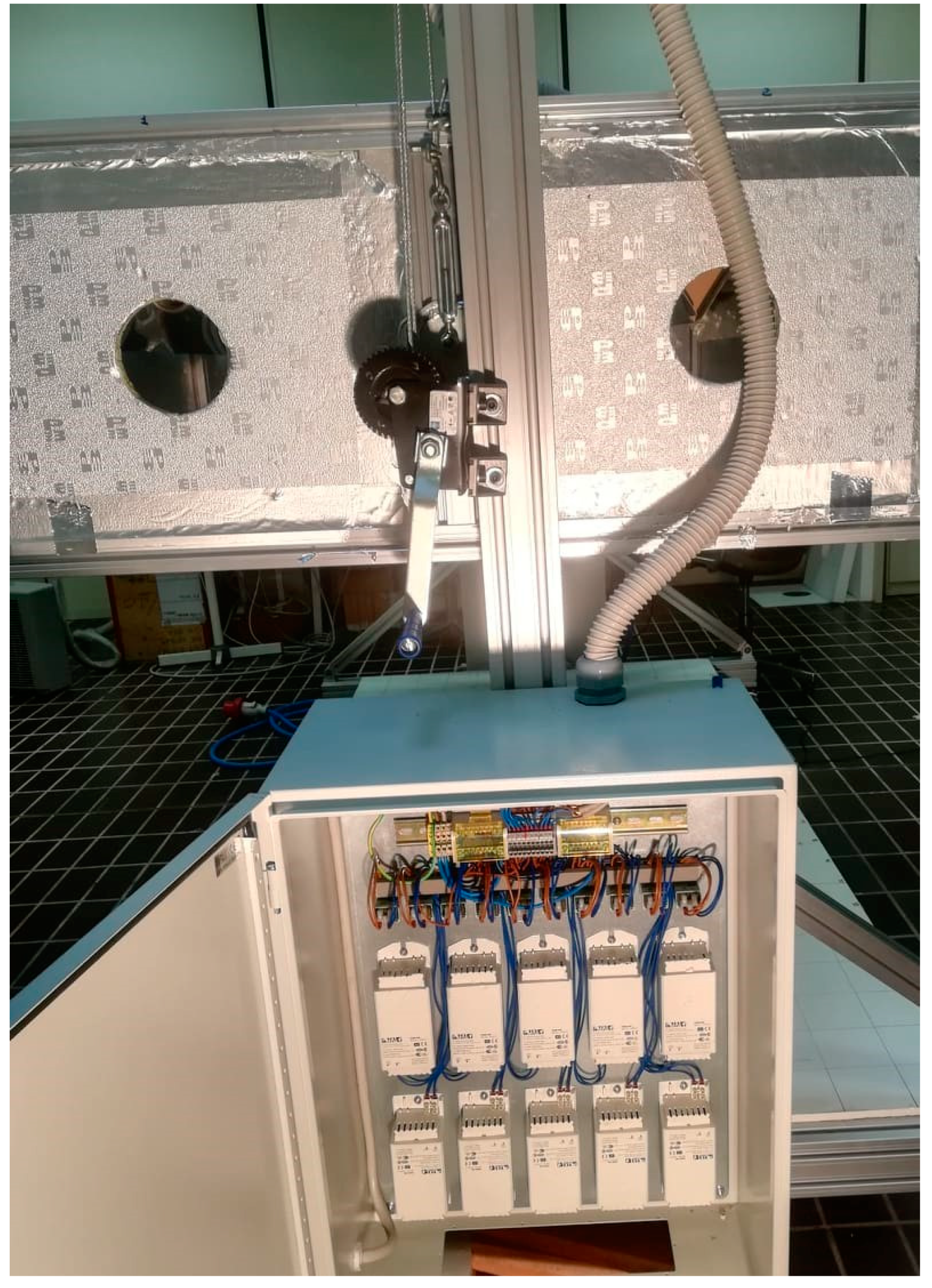
The electrical panels are located on the sides of the structure and are cooled by fans (Figure 5). The lamps are powered by a three-phase system. Each 220 V phase has an associated neutral phase; the first two phases feed a group of seven lamps each, while the third phase feeds the remaining six lamps. The 20 lamps are connected to the side boxes in two groups of 10, that is, a phase of seven plus three of the phase of six lamps. The parabola arrangement is not symmetrical with respect to the center of the structure, as the pulley is mounted for the handling of lamps.
3. Results
A series of tests were carried out according to the IEC 60904-9 standard, “Solar simulator performance requirements”, namely nonuniformity of irradiance and temporal instability. These are useful parameters to define if a solar simulation meets the requirements of Class A, B, or C, the ranges of which are defined in Table 1. The experiments were carried out in the Department of “Industrial Engineering and Mathematical Sciences” of the Polytechnic University of Marche in Ancona (Italy).
3.1. Radiation Nonuniformity
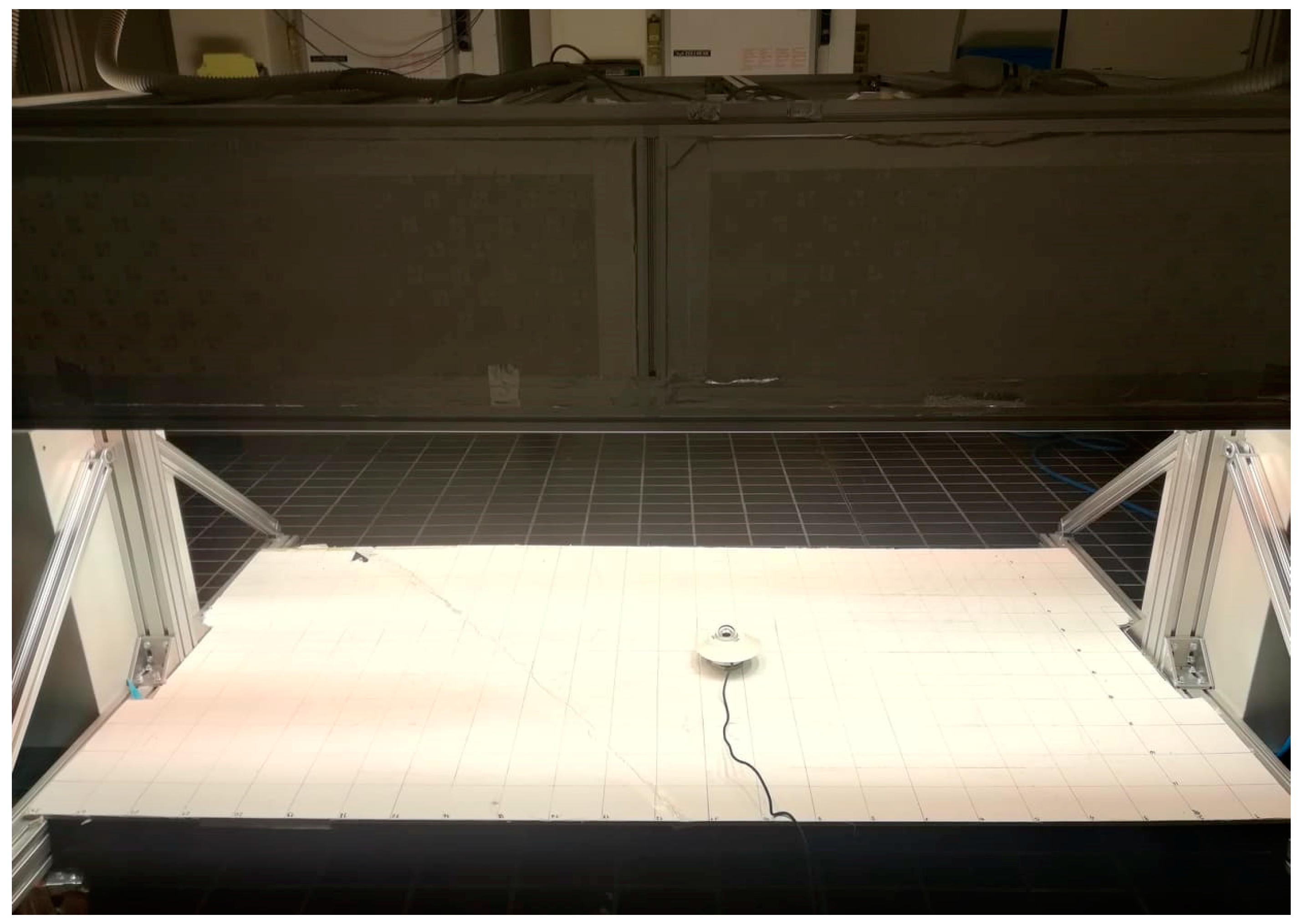
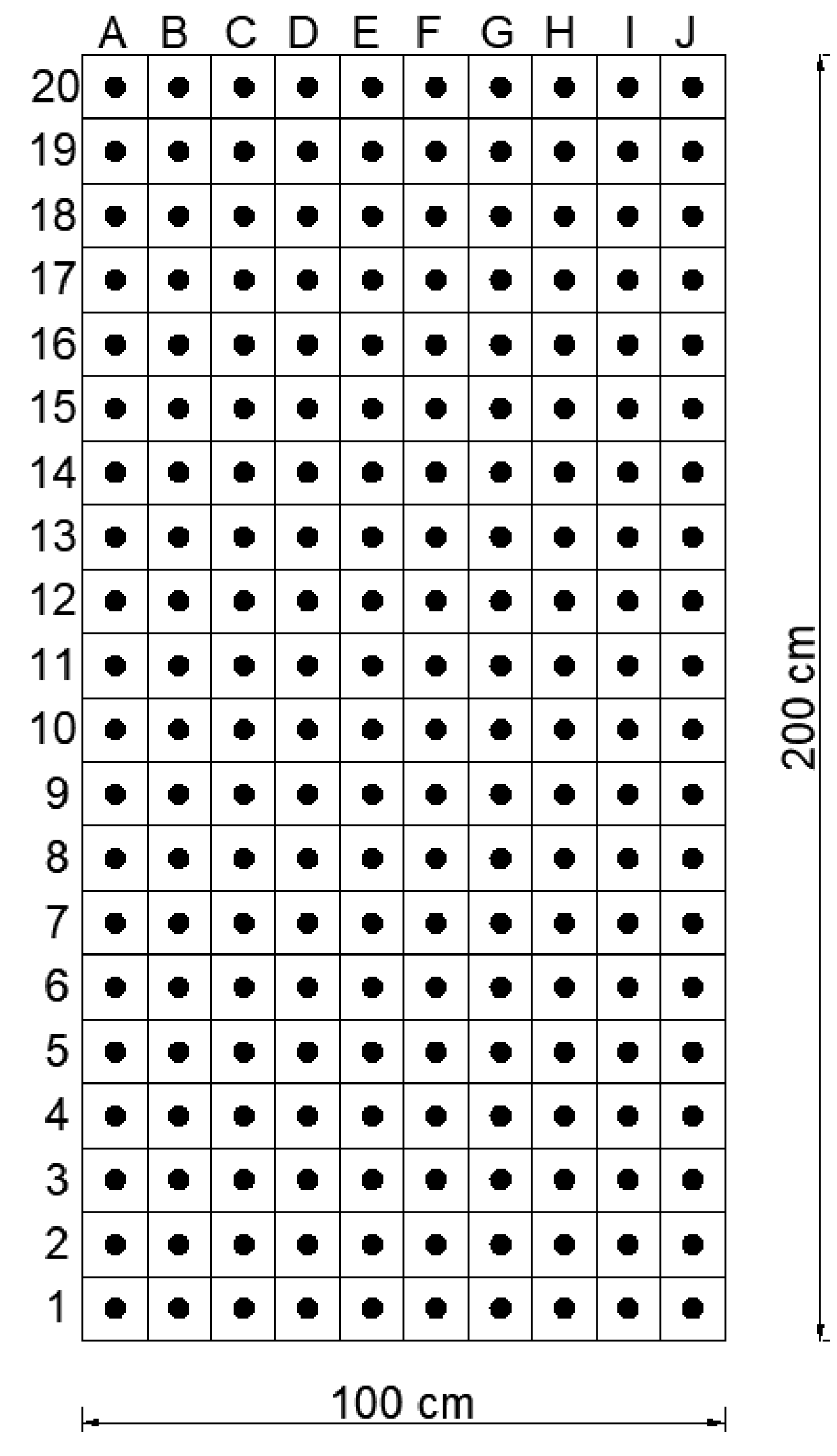
In the experimental stage, the spatial uniformity was investigated by evaluating the irradiance on the test surface of the solar simulator. A pyranometer, model DPA/ESR 154, was used to measure the global solar radiation on the test surface. The device can measure from 0 to 2000 W/m2, with a sensitivity of 10.88 µV/Wm−2, a linearity of 0.75%, and a sampling time of 1 s. The target area was divided into 200 squares, each with a side of 10 cm. The irradiation was thoroughly measured by moving the pyranometer inside the rectangular grid. The pyranometer was positioned in the center of each square. The total measured area is 200 × 100 cm (Figure 6). Data were acquired with the National Instrument NI-9205, a module for the acquisition of input voltage. The measured signal was converted from mV to W/m2 in the software LabVIEW to have a more understandable graph. Figure 7 shows the arrangement of the measuring points, from position A1 to J20. The irradiance was assumed to be constant during the entire testing process because of the generally constant electrical alimentation.
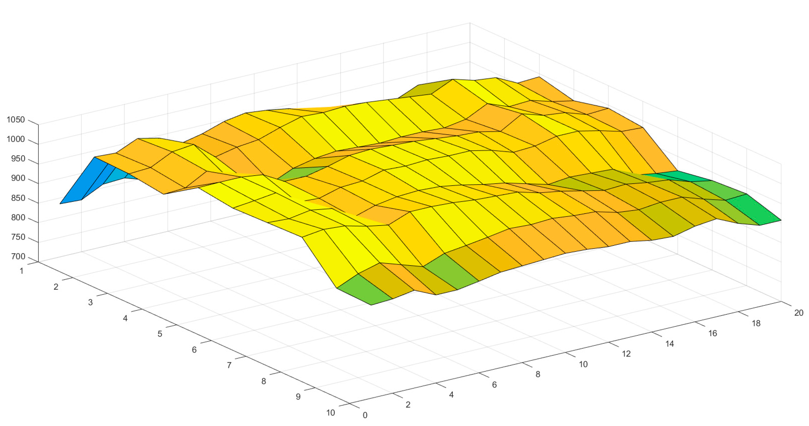
Figure 8 shows the results over the entire test area.
According to the IEC 60904-7 standard, the nonuniformity is defined by the following equation:
where Emax is the maximum irradiance measured by detector (in W/m2) and Emin is the minimum irradiance (in W/m2).
The highest measured value on the test area was about 1038 W/m2 at the positions C5, E19, and H19, and the lowest was equal to 729 W/m2 at the position A1. With the results of the experimental tests, the classes in the test area can be determined in accordance with the quality standards. Table 2 lists the percentage error deviation from the maximum irradiation for the three classes. In particular, Class C (depicted by the blue rectangle) consists of the area that spans from B20 to J1, with a dimension of 200 × 90 cm, and the Class B (depicted by the red rectangle) area spans from cell B20 to cell I4, with a dimension of 170 × 80 cm.
The Class A area is composed of the cells ranging from E17 to H10, considering its relative maximum in cell E17 equal to 1031 W/m2 (Table 3). It has an area of 80 × 40 cm. The asymmetric position of the rectangles is due, as described above, to the slight displacement of the parabolas for the mounting of the pulley. Table 4 summarizes the dimensions of the three classes obtained, showing the maximum, the minimum and the average value in each of them.
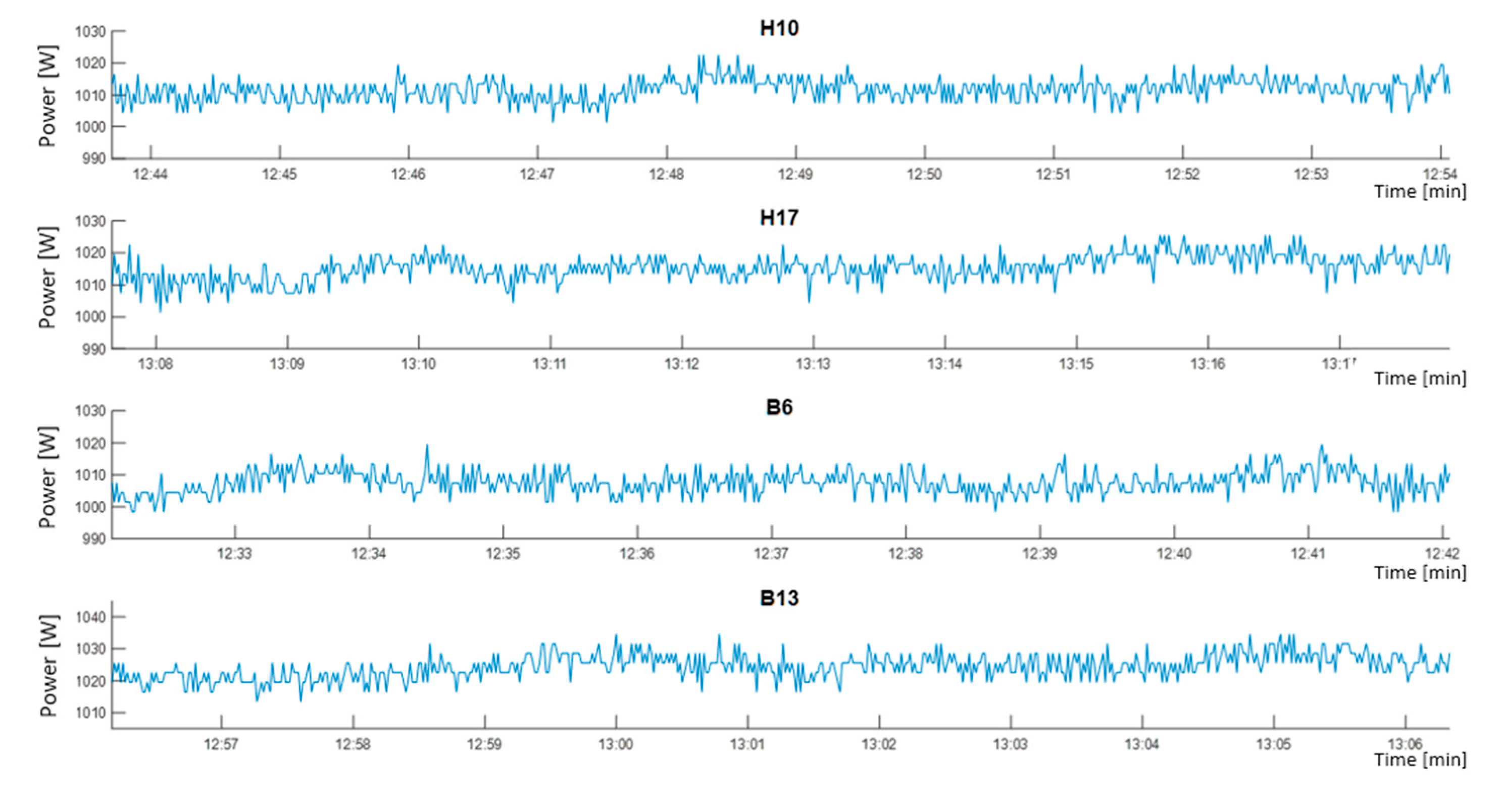
3.2. Radiation Instability over Time
In accordance with IEC 60904-9, the test comprises a long-term irradiation measurement in a specific point on the test surface for a time equal to 10 min. The lamps require a warm-up time to reach the nominal power (approximately 3 min). The irradiance value was controlled and maintained constant at 1000 W/m2 for the entire duration of the test.
The temporal instability is given by the following equation:
where is the maximum irradiance at the selected point during the test and is the minimum irradiance at the same point, both measured in W/m2.
On the test area, four specific points were selected to test the temporal instability: H10, H17, B6, and B13. During the 10-min test, the maximum and the minimum irradiance values were recorded, and the percentage error was calculated by Equation (3). Table 5 summarizes the results, and all the measured points meet the Class A standards since the error is less than 2%. Figure 9 shows the complete trends.
3.3. I–V Curve
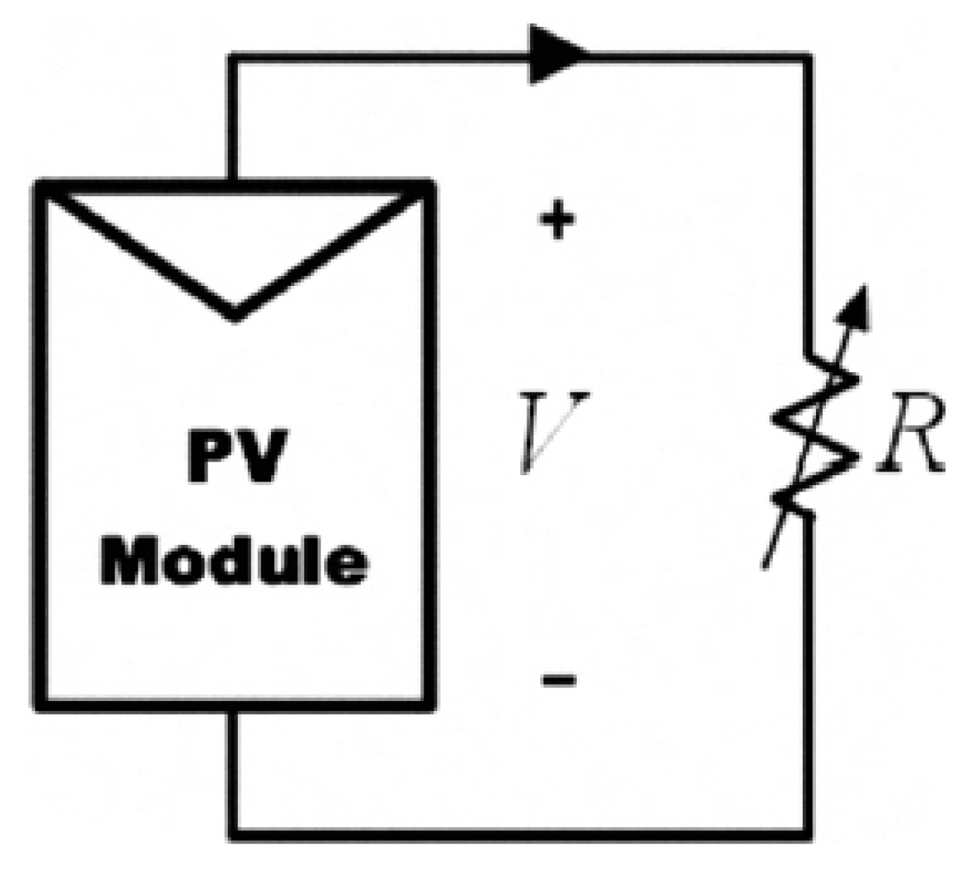
Further investigation was conducted by characterizing the I–V curve of a PV panel. The experimental analysis was carried out with tests performed under the artificial radiation and with tests outside with natural solar radiation. The panel was connected to a variable resistor, and the curve was obtained by varying the value of the resistance from zero to infinity [24] (Figure 10). In each step, the voltage and the current were simultaneously measured. A 40 W 12 V panel with monocrystalline cells was chosen, with dimensions of 650 × 505 × 30 mm. The module voltage (Vmp) was 17.8 V, the nominal current (Imp) was 2.3 A, the short-circuit current (Isc) was 2.7 A, and the open-circuit voltage (Voc) was 21.3 V. The panel was composed of 36 cells.
To validate the experimental results, a numerical method was implemented on the software MATLAB. The relationship between voltage and current is as follows [25]:
where Isc,TG and Voc,TG are the short-circuit current and the open-circuit voltage at a given temperature (T) and solar irradiance (G), respectively, and s is the shape parameter.
The temperature and voltage dependence of Isc and Voc parameters are the following:
where STC indicates standard test conditions (cell temperature equal to 25 °C, solar irradiance equal to 1000 W/m2 and an average solar spectrum at air mass AM1.5), µIsc and µVoc are the current–temperature and voltage–temperature coefficients, respectively; Ns is the number of solar cells of the PV panel; and Vt,T is the thermal voltage given by Equation (9) as a function of the cell temperature, the Boltzmann constant, and the value of the electron charge [26]:
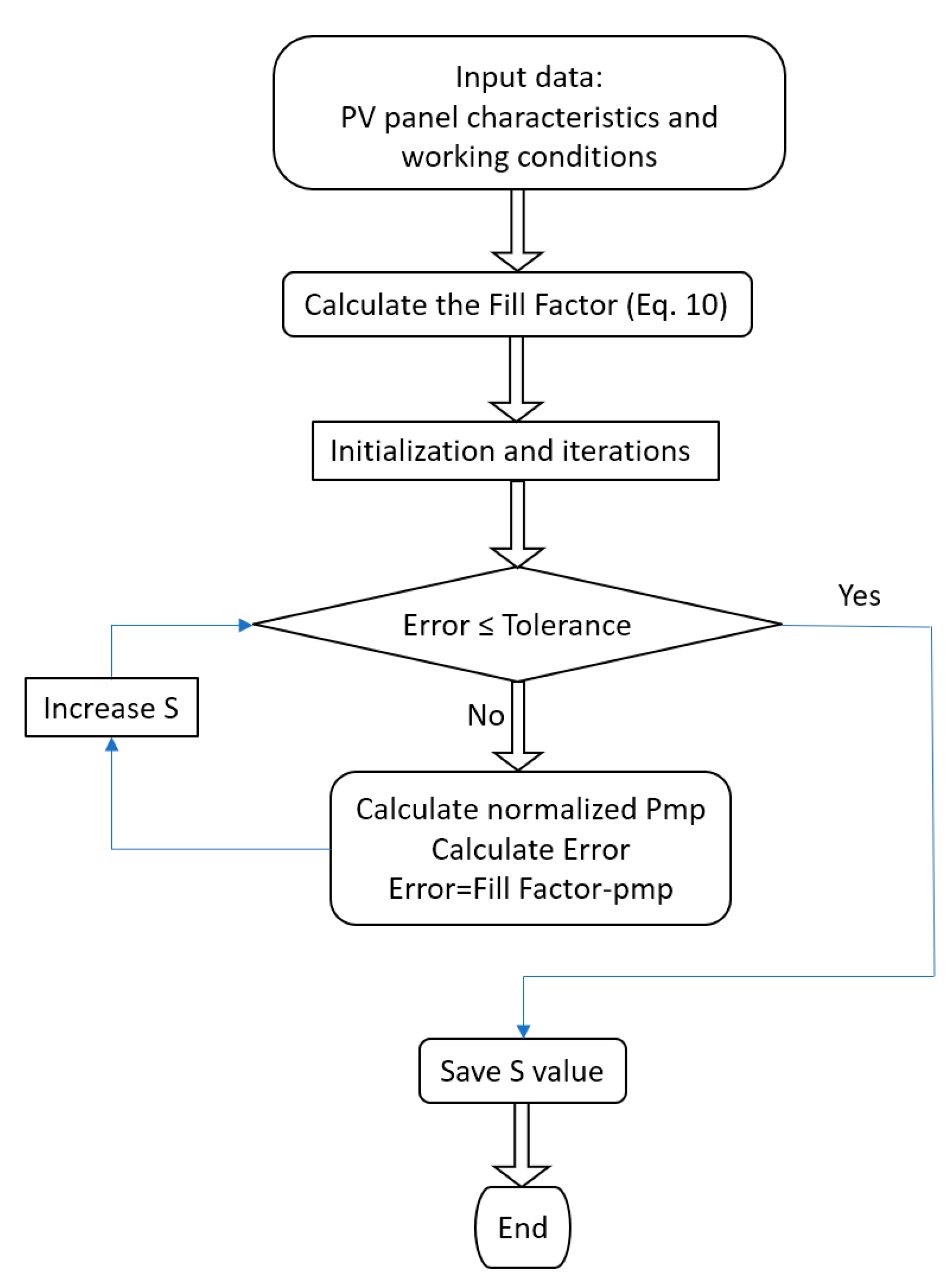
Iterations are required to determine the shape parameter s. The value is initially set to 1, and it is increased by a fixed amount after each iteration. The procedure ends when the difference (called error) between the fill factor and the normalized electric power is less than the tolerance established at the beginning. The flowchart is summarized in Figure 11 [25].
A valid expression for the fill factor FFtg(T,G) is given by [27]
with FF0 [28]:
and
where
where FF0 is the fill factor of the ideal PV without resistive effects, rs is the normalized series resistance, voc,t is the normalized thermal voltage, n is the diode quality factor, Rs is the internal resistance, and FF is the fill factor at STC conditions.
Figure 12 compares the three curves. The simulated solar radiation curve shows a good approximation when compared to the curves of both the outdoor experiment and the numerical method.
4. Conclusions
A metal halide solar simulator for indoor applications is presented in this work. The optical system based on parabolic reflection proves to be a good choice because lamps can be arranged in a matrix pattern and obtain the same flux conditions. This way, a large target surface can be obtained. The disadvantage is that parabolas require a high degree of precision during their construction to obtain the exact shape designed in the theoretical phase. Furthermore, in the assembly phase, a perfect contact between the aluminum parabola and the wooden forms must be guaranteed. An additional advantage is the mobile structure of the solar simulator because it grants light intensity regulation to reproduce, for instance, daily irradiance profiles and the testing of devices under a desirable incidence angle. Spatial uniformity and temporal stability tests provided excellent results. Classes C, B, and A were obtained on the test planes of 200 × 90 cm, 170 × 80 cm, and 80 × 40 cm, respectively. The temporal instability test met Class A standards for all the measured points. In the I–V curve characterization of a PV panel, the results are very similar to those obtained with the external test under natural radiation and with a software-implemented numerical method. Further improvements in realizing a larger target area and extending the spectrum in the infrared and UV area can be investigated. This can be achieved by adding infrared or UV emitters in the right amount, position, and power in the already present lamp array.
Author Contributions
Conceptualization, D.C., P.P. and R.F.; Investigation, D.C., E.T. and R.F.; Methodology, D.C., E.T., P.P. and R.F.; Software, D.C.; Supervision, P.P.; Validation, D.C., E.T. and P.P.; Writing – original draft, D.C. and E.T.; Writing – review & editing, D.C. and P.P. All authors have read and agreed to the published version of the manuscript.
Funding
This research received no external funding.
Institutional Review Board Statement
Not applicable.
Informed Consent Statement
Not applicable.
Conflicts of Interest
The authors declare no conflict of interest.
References
- Moss, R.W.; Shire, G.S.F.; Eames, P.C.; Henshall, P.; Hyde, T.; Arya, F. Design and commissioning of a virtual image solar simulator for testing thermal collectors. Sol. Energy 2018, 159, 234–242. [Google Scholar]
- Kongtragool, B.; Wongwises, S. A four power-piston low-temperature differential Stirling engine using simulated solar energy as a heat source. Sol. Energy 2008, 82, 493–500. [Google Scholar]
- Decker, A.J.; Pollack, J.L. A 400 kW Argon Arc Lamp for Solar Simulation; Space Simulation Conference: New York, NY, USA, 1972. [Google Scholar]
- Codd, D.S.; Carlson, A.; Rees, J.; Slocum, A.H. A low cost high flux solar simulator. Sol. Energy 2010, 84, 2202–2212. [Google Scholar]
- Meng, Q.; Wang, Y.; Zhang, L. Irradiance characteristics and optimization design of a large-scale solar simulator. Sol. Energy 2011, 85, 1758–1767. [Google Scholar]
- Dibowski, G.; Eber, K. Hazards caused by UV rays of xenon light based high performance solar simulators. Saf. Health Work 2017, 8, 237–245. [Google Scholar]
- Song, J.; Wang, J.; Niu, Y.; Wang, W.; Tong, K.; Yu, H.; Yang, Y. Flexible highflux solar simulator based on opticalfiber bundles. Sol. Energy 2019, 193, 576–583. [Google Scholar]
- Kolberg, D.; Schubert, F.; Lontke, N.; Zwigart, A.; Spinner, D.M. Development of tunable close match LED solar simulator with extended spectral range to UV and IR. Energy Procedia 2011, 8, 100–105. [Google Scholar]
- Tavakoli, M.; Jahantigh, F.; Zarookian, H. Adjustable high-power-LED solar simulator with extended spectrum in UV region. Sol. Energy 2020. [Google Scholar] [CrossRef]
- Watjanatepin, N. Design construct and evaluation of six-spectral LEDs-based solar simulator based on IEC 60904–9. Int. J. Eng. Technol. 2017, 9, 923–931. [Google Scholar]
- Georgescu, A.; Damache, G.; Gîrţu, M.A. Class A small area solar simulator for dye-sensitized solar cell testing. J. Optoelectron. Adv. Mater. 2008, 10, 3003–3007. [Google Scholar]
- Leary, G.; Switzer, G.; Kuntz, G.; Kaiser, T. Comparison of xenon lamp-based and led-based solar simulators. In Proceedings of the IEEE 43th Photovoltaic Specialist Conference, Portland, OR, USA, 5–10 June 2017; pp. 1–6. [Google Scholar]
- Esen, V.; Saglam, S.; Oral, B.; Esen, O.C. Spectrum measurement of variable irradiance controlled LED-based solar simulator. Int. J. Renew. Energy Res. 2020, 10, 109–116. [Google Scholar]
- Sabahi, H.; Tofigh, A.A.; Kakhki, I.M.; Bungypoor-Fard, H. Design, construction and performance test of an efficient large-scale solar simulator for investigation of solar thermal collectors. Sustain. Energy Technol. Assess. 2016, 15, 35–41. [Google Scholar]
- ASTM Standard G173-03. Standard Tables for Reference Solar Spectral Irradiances: Direct Normal and Hemispherical on 37° Tilted Surface; West Conshohocken, PA, USA, 2012. [Google Scholar]
- ISO 9806. Solar Energy. Solar Thermal Collectors. Test Methods; British Standards Institute: London, UK, 2013. [Google Scholar]
- Holmberg, J.; Flynn, C.; Portinari, L. The colours of the Sun. Mon. Not. R. Astron. Soc. 2006, 367, 449–453. [Google Scholar]
- ISO 19467. Thermal Performance of Windows and Doors—Determination of Solar Heat Gain Coefficient Using Solar Simulator; British Standards Institute: London, UK, 2016. [Google Scholar]
- EN 12975-1. Thermal Solar Systems and Components—Solar Collectors—Part 1: General Requirements; British Standards Institute: London, UK, 2006. [Google Scholar]
- EN 12976-1. Thermal Solar Systems and Components—Factory Made Systems—Part 1: General Requirements; British Standards Institute: London, UK, 2017. [Google Scholar]
- IEC 60904-9. Photovoltaic Devices—Part 9: Solar Simulator Performance Requirements. Geneva: IEC; International Electrotechnical Commission, 2007. [Google Scholar]
- Philips. Product Datasheet: MASTER Colour CDM-T MW eco/360 W842 E40. Available online: http://www.lighting.philips.it/api/assets/v1/file/content/fp928070319230-pss-it_it/928070319230_EU.it_IT.PROF.FP.pdf (accessed on 29 July 2020).
- Tawfik, M.; Tonnellier, X.; Sansom, C. Light source selection for a solar simulator for thermal application: A review. Renew. Sustain. Energy Rev. 2018, 90, 802–813. [Google Scholar]
- Duran, E.; Piliougine, M.; Sidrach-de-Cardona, M.; Galan, J.; Andujar, J.M. Different methods to obtain the I–V curve of PV modules: A review. In Proceedings of the 2008 33th IEEE Photovoltaic Specialists Conference, San Diego, CA, USA, 11–16 May 2008; pp. 1–6. [Google Scholar]
- Boutana, N.; Mellit, A.; Haddad, S.; Rabhi, A.; Pavan, A.M. An explicit IV model for photovoltaic module technologies. Energy Convers. Manag. 2017, 138, 400–412. [Google Scholar]
- Nassar-eddine, I.; Obbadi, A.; Errami, Y.; Agunaou, M. Parameter estimation of photovoltaic modules using iterative method and the Lambert W function: A comparative study. Energy Convers Manag. 2016, 119, 37–48. [Google Scholar]
- Green, M.A. Solar cell fill factors: General graph and empirical expressions. Solid State Electron 1981, 24, 788–789. [Google Scholar]
- Pavan, A.; Mellit, A.; de Pieri, D.; Lughi, V. A study on the mismatch effect due to the use of different photovoltaic modules classes in large-scale solar parks. Prog. Photovolt. Res. Appl. 2014, 22, 332–345. [Google Scholar]
Figure 1.
Metal halide lamp structure (mm).

Figure 2.
Detail of a lamp mounted under the parabolic mirror (a) and the theoretical representation (b).
Figure 2.
Detail of a lamp mounted under the parabolic mirror (a) and the theoretical representation (b).

Figure 3.
Lamp array size. CAD reconstruction (mm) (a) and real image (b).

Figure 4.
3D view of the whole system: vertical flux configuration (a) and horizontal flux configuration (b).
Figure 4.
3D view of the whole system: vertical flux configuration (a) and horizontal flux configuration (b).

Figure 5.
Detail of a side box.

Figure 6.
Nonuniformity test (the shadows are due to the photo).

Figure 7.
Layout of the test area.

Figure 8.
Spatial distribution of irradiation values on the test surface (W/m2).

Figure 9.
Long-term instability test results.

Figure 10.
Variable resistor scheme [24].
Figure 10.
Variable resistor scheme [24].

Figure 11.
Procedure for the determination of the shape S parameter [25].
Figure 11.
Procedure for the determination of the shape S parameter [25].

Figure 12.
Comparison of indoor, outdoor, and numerical I–V curve.


Table 1.
Classification of solar simulator performance.
| Characteristics | Class A | Class B | Class C |
|---|---|---|---|
| Nonuniformity | ≤2% | ≤5% | ≤10% |
| Temporal instability | ≤2% | ≤5% | ≤10% |
Table 2.
The percentage error of irradiation. The blue rectangle indicates the Class C standard area obtained, the red one the Class B.
Table 2.
The percentage error of irradiation. The blue rectangle indicates the Class C standard area obtained, the red one the Class B.
 |
Table 3.
Individuation of Class A area in test surface.
| E | F | G | H | |
|---|---|---|---|---|
| 17 | 0.0% | 1.5% | 0.3% | 0.5% |
| 16 | 1.5% | 1.6% | 2.0% | 1.0% |
| 15 | 1.5% | 0.9% | 1.2% | 0.0% |
| 14 | 0.9% | 0.7% | 0.7% | 0.0% |
| 13 | 0.1% | 0.0% | 0.6% | 0.1% |
| 12 | 0.0% | 0.1% | 0.7% | 0.4% |
| 11 | 0.1% | 0.0% | 1.2% | 0.6% |
| 10 | 0.3% | 0.1% | 1.8% | 0.7% |
Table 4.
Class parameters in testing area.
| Class A | Class B | Class C | |
|---|---|---|---|
| Definition area | From E17 to H10 | From B20 to I4 | From B20 TO J1 |
| Dimension area [cm] | 80 × 40 | 170 × 80 | 200 × 90 |
| Max relative [W/m2] | 1031 | 1038 | 1038 |
| Min relative [W/m2] | 990 | 925 | 919 |
| Average [W/m2] | 1017 | 995 | 993 |
Table 5.
Long-term instability values at a specific point.
| Cell Number | Max Irradiance [W] | Min Irradiance [W] | Error [%] | Class |
|---|---|---|---|---|
| H10 | 1022.5 | 1001.3 | 1.04% | A |
| H17 | 1025.5 | 1001.3 | 1.19% | A |
| B6 | 1034.5 | 1113.4 | 1.03% | A |
| B13 | 1019.4 | 998.8 | 1.04% | A |
Publisher’s Note: MDPI stays neutral with regard to jurisdictional claims in published maps and institutional affiliations. |
© 2021 by the authors. Licensee MDPI, Basel, Switzerland. This article is an open access article distributed under the terms and conditions of the Creative Commons Attribution (CC BY) license (http://creativecommons.org/licenses/by/4.0/).
Share and Cite
MDPI and ACS Style
Colarossi, D.; Tagliolini, E.; Principi, P.; Fioretti, R. Design and Validation of an Adjustable Large-Scale Solar Simulator. Appl. Sci. 2021, 11, 1964. https://0-doi-org.brum.beds.ac.uk/10.3390/app11041964
AMA Style
Colarossi D, Tagliolini E, Principi P, Fioretti R. Design and Validation of an Adjustable Large-Scale Solar Simulator. Applied Sciences. 2021; 11(4):1964. https://0-doi-org.brum.beds.ac.uk/10.3390/app11041964
Chicago/Turabian StyleColarossi, Daniele, Eleonora Tagliolini, Paolo Principi, and Roberto Fioretti. 2021. "Design and Validation of an Adjustable Large-Scale Solar Simulator" Applied Sciences 11, no. 4: 1964. https://0-doi-org.brum.beds.ac.uk/10.3390/app11041964
Note that from the first issue of 2016, this journal uses article numbers instead of page numbers. See further details here.