Impact of the Sub-Grid Scale Turbulence Model in Aeroacoustic Simulation of Human Voice

Abstract

In an aeroacoustic simulation of human voice production, the effect of the sub-grid scale (SGS) model on the acoustic spectrum was investigated. In the first step, incompressible airflow in a 3D model of larynx with vocal folds undergoing prescribed two-degree-of-freedom oscillation was simulated by laminar and Large-Eddy Simulations (LES), using the One-Equation and Wall-Adaptive Local-Eddy (WALE) SGS models. Second, the aeroacoustic sources and the sound propagation in a domain composed of the larynx and vocal tract were computed by the Perturbed Convective Wave Equation (PCWE) for vowels [u:] and [i:]. The results show that the SGS model has a significant impact not only on the flow field, but also on the spectrum of the sound sampled 1 cm downstream of the lips. With the WALE model, which is known to handle the near-wall and high-shear regions more precisely, the simulations predict significantly higher peak volumetric flow rates of air than those of the One-Equation model, only slightly lower than the laminar simulation. The usage of the WALE SGS model also results in higher sound pressure levels of the higher harmonic frequencies.

1. Introduction

Generation of the human voice is a highly complex biophysical process, where the viscoelastic multi-layered tissues of the vocal folds interact with the airflow expired from the lungs, start to self-oscillate and close the channel periodically. The vocal fold oscillation and glottal closure modulate the mass flux, create complex turbulent structures and pressure disturbances, which form the voice source. This source signal is modulated by the vocal tract, radiated from the mouth, and is perceived as a human voice. The physiological principles are well described in the monograph by Titze [1].

The acoustic resonances of the subglottal spaces (trachea, bronchi, and bronchioles) and supraglottal part (the vocal tract) can enhance the driving pressures of the vocal folds and the glottal flow, thereby modifying the energy level of sound sources. The voice generation is governed by a three-way interaction between the structure, airflow and acoustics. The dominant aeroacoustic sound sources are located within the glottis and the supraglottal region. Three characteristics of flow-induced sound are defined in terms of free-field radiation—first, vocal fold oscillation induces a monopole radiation pattern. Second, the interaction of the vocal folds and the air jet creates surface pressure fluctuations that radiate like a dipole. Third, the turbulent structures located downstream of the glottal constriction have a quadrupolar radiation pattern [2,3]. The sound due to turbulence has a significant influence on the broadband noise at higher frequencies.

The principles of voice generation may be studied by in vivo, excised larynx or synthetic vocal fold measurements [4,5], or by numerical modelling. During recent decades, numerical simulation of human phonation has advanced considerably towards a state where full-scale aeroacoustic simulations on realistic computed tomography (CT)- or magnetic resonance imaging (MRI)-based geometries are possible. It can be anticipated that soon these simulations could be used for subject-specific pre-surgical predictions of vocal fold oscillations and resulting voice quality for people suffering from various vocal fold dysfunctions [6,7] or for the development of vocal fold prostheses. However, though powerful numerical simulation tools are available, the numerical methods still face challenges due to the nonlinear phenomena both in solid and fluid mechanics. This study focuses on the impact of the numerical approach to turbulence modeling on the aeroacoustic simulation of voice generation.

Turbulence is an inherent property of medium and high Reynolds number flows, where the energy of the large flow structures is transferred in a cascade of scales towards the smallest vortices, where the turbulent kinetic energy dissipates into heat. Measurements on excised canine larynges suggest that the airflow in trachea, subglottal and intraglottal space is typically laminar, but encounters transition to turbulence shortly downstream of the glottis [8,9,10]. The vortex dynamics in the supraglottal spaces and vocal tract are governed by turbulent momentum transfer. Turbulence also induces a broadband sound source, which is important especially in the case of breathy phonation, but is also significant in the case of modal voice [11].

In the computational fluid dynamics (CFD) of turbulent flows, three approaches are used. First, the Direct Numerical Simulations (DNS), that is, straightforward discretization of the Navier-Stokes equations on a sufficiently fine computational mesh, where all turbulent scales up to the smallest dissipating vortices are resolved. Even for moderate Reynolds numbers encountered in laryngeal airflow, this type of simulation is prohibitively expensive in terms of computational requirements. Sometimes, the term “laminar simulation” is, somewhat incorrectly, used for a DNS of flow using a coarse mesh. This is correct for purely laminar flow with no turbulence. However, using the “laminar” model for turbulent flow, actually, a DNS on a coarse grid unable to capture the small-scale fluid motions, introduces error since the influence of the sub-grid vortices on the large-scale (resolved) turbulent motions is neglected. The second approach is the current industry standard, unsteady Reynolds-Averaged Navier-Stokes equations (RANS), which completely gives up resolving the turbulent fluctuations and dynamic evolution of vortical structures, and aims to calculate the mean, time-averaged flow. The influence of turbulence on the mean flow is modeled using some of the plethoras of more or less complex turbulence models. Clearly, RANS is unsuitable for aeroacoustic simulations of voice where the unsteady turbulent motions represent a crucial portion of the aeroacoustic sources.

With rigorous DNS being infeasible and RANS inapplicable, numerical modeling of the aeroacoustic principles of voice production can use either the laminar simulations (such as in [12,13,14,15,16,17,18,19,20]) or the third, arguably most promising approach—the Large Eddy Simulation (LES). LES may be regarded as a compromise between RANS, where the entire effect of turbulence is modeled, and DNS, where all the turbulent scales are resolved. The LES concept resolves the large, anisotropic energy-carrying fluid motions and models the effect of sub-grid scale, largely isotropic turbulent structures. Large Eddy Simulations are still computationally expensive, especially if the boundary layer is to be resolved properly. However, current parallel computational resources make this approach viable for low and moderate Reynolds-number flows. In the numerical simulation of human phonation, the LES approach has been used in recent years. One of the first was the work of Suh and Frankel [21], who used compressible LES and Ffowcs Williams-Hawkings acoustic analogy in a static model of human glottis for far-field sound predictions. The work by Mihaescu [22,23] employed the LES capability of ANSYS Fluent (ANSYS, Canonsburg, PA/USA) to study the laryngeal airflow both during phonation and inspiration. The work of Schwarze et al. [24] explores a variant called Implicit LES, where the intrinsic dissipation of the numerical method is assumed to act as a sub-grid scale (SGS) model. Another compressible LES simulation on a static glottis was published by de Luzan et al. [25]. Recently, Sadeghi [6,7,26] simulated the laryngeal flow and effect of ventricular folds using the LES feature of STAR-CCM+ (Siemens PLM Software, Plano, TX/USA) and quantified the computational requirements on parallel architectures. In the study by Schickhofer et al. [27], the same software and similar numerical approach was used to study the influence of the supraglottal coherent structures produced by flow through static glottis on the far-field sound signal on a realistic vocal tract geometry from MRI data.

A systematic comparison of the airflow and sound generated in human larynx, obtained using laminar and LES flow simulations, should help to assess the importance and impact of turbulence modeling in aeroacoustic simulations of voice generation. This study builds on the previous publications [18,28] and compares the acoustic spectra obtained using a laminar simulation (i.e., with no SGS modeling) and two variants of Large Eddy Simulations with different sub-grid scale models—the One-Equation Eddy-Viscosity SGS model [29] and the Wall-Adaptive Local Eddy-Viscosity (WALE) model [30]. The impact of the sub-grid scale model on the spectrum of the generated voice for vowels [u:] and [i:] is analyzed and discussed.

This paper is organized into two major sections, describing the fluid dynamic and aeroacoustic models. Section 2.1 explains the Large Eddy Simulation framework, SGS models used and boundary conditions of the mathematical model. This is followed by Section 2.3 and Section 2.4 on the geometry, mesh and numerical solution of the CFD problem, and eventually Section 2.5 presents the results of the CFD simulations. Section 3 has a similar structure, explaining first the mathematical model, then the numerical approach and finally the presenting the results of the aeroacoustic simulations.

2. CFD Model of Incompressible Flow in the Larynx

2.1. Mathematical Model

Large Eddy Simulation is a mathematical concept for modeling turbulent flows, which deals with flow structures carrying most kinetic energy, that is, spatially organized large scales. These consist of two main categories: coherent structures and coherent vortices of recognizable shape [31]. In the numerical implementation, the characteristic length $\Delta$, defining a cutoff between resolved scales and modeled sub-grid scales, is usually given by the mesh grid spacing [32].

In the LES concept, any flow variable $f(\mathit{x},t)$, where $\mathit{x}=(x_1,x_2,x_3)$ is the spatial coordinate and t time, may be decomposed as

$$f(\mathit{x},t)=\overline{f}(\mathit{x},t)+f^{\prime }(\mathit{x},t),$$

(1)

where $\overline{f}(\mathit{x},t)=G\left(\mathit{x}\right)\ast f(\mathit{x},t)=\int G(\mathit{r},\mathit{x},\Delta )f(\mathit{x}-\mathit{r},t)d\mathit{r}$ is the large-scale component, obtained by spatial filtering, and $f^{\prime }(x,t)$ is the small, sub-grid scale contribution. The convolution introduced above contains a filter function G separating spatial scales $\left|\mathit{r}\right|\le \Delta /2$ from $\left|\mathit{r}\right|>\Delta /2$. In current simulations, a top-hat filter is used, which is a common choice in low-order finite volume methods. The effect of sub-grid scale (SGS) contributions on the large flow scales relies on the assumption of isotropic (non-directional) small-scale turbulence and is modeled.

The continuity and momentum equations for the incompressible fluid flow, with LES filtering applied, can be written as

$$\frac{\partial {\overline{U}}_i}{\partial x_i}=0,$$

(2)

$$\frac{\partial {\overline{U}}_i}{\partial t}+\frac{\partial }{\partial x_j}\left(\overline{U_i{U}_j}\right)=-\frac{1}{\rho }\frac{\partial \overline{p}}{\partial x_i}+\nu \frac{{\partial }^2{\overline{U}}_i}{\partial x_j\partial x_j},$$

(3)

where ${\overline{U}}_i$ is the filtered velocity, $\overline{p}$ represents the filtered static pressure and $\nu =1.58·{10}^{-5}{\mathrm{m}}^2{\mathrm{s}}^{-1}$ is the kinematic molecular viscosity. The term $\overline{U_i{U}_j}$ is the dyadic product and cannot be expressed directly [33]. Modification of the momentum Equation (3) by $+\frac{\partial }{\partial x_j}\left({\overline{U}}_i{\overline{U}}_j\right)$ yields

$$\frac{\partial {\overline{U}}_i}{\partial t}+\frac{\partial }{\partial x_j}\left({\overline{U}}_i{\overline{U}}_j\right)=-\frac{1}{\rho }\frac{\partial \overline{p}}{\partial x_i}+\nu \frac{{\partial }^2{\overline{U}}_i}{\partial x_j\partial x_j}-\frac{\partial {\tau }_{ij}}{\partial x_j}.$$

(4)

The new term on the right-hand side of (4) is the divergence of the sub-grid scale (SGS) stress tensor

$${\tau }_{ij}=\overline{U_i{U}_j}-{\overline{U}}_i{\overline{U}}_j=-(\overline{u_i^{{}^{\prime }}{u}_j^{{}^{\prime }}}+\overline{\overline{U_i}{u}_j^{{}^{\prime }}}+\overline{u_i^{{}^{\prime }}{\overline{U}}_j}+\overline{{\overline{U}}_i{\overline{U}}_j}-{\overline{U}}_i{\overline{U}}_j),$$

(5)

where the individual tensors are $-\overline{u_i^{{}^{\prime }}{u}_j^{{}^{\prime }}}$ the Reynolds-stress-like term, $-(\overline{\overline{U_i}{u}_j^{{}^{\prime }}}+\overline{u_i^{{}^{\prime }}\overline{U_j}})$ the Clark term [34] and $-(\overline{\overline{U_i}\overline{U_j}}+{\overline{U}}_i{\overline{U}}_j)$ the Leonard term [35]. The SGS stress tensor is left to be modeled to close the set of equations. Compared to the Reynolds stresses in RANS, the SGS stresses carry much less of the turbulent energy, and so the accuracy of the model is less important.

2.1.1. Smagorinsky SGS Model

One of the first and simplest SGS models was the Smagorinsky algebraic model [36], based on the eddy-viscosity assumption, which states that the deviatoric part of the SGS stress tensor is proportional to the symmetric part of the velocity gradient tensor ${\overline{S}}_{ij}=\frac{1}{2}\left(\partial {\overline{U}}_i/\partial x_j+\partial {\overline{U}}_j/\partial x_i\right)$:

$${\tau }_{ij}-\frac{1}{3}{\tau }_{kk}{\delta }_{ij}=-2{\nu }_t{\overline{S}}_{ij}=-{\nu }_t\left(\frac{\partial {\overline{U}}_i}{\partial x_j}+\frac{\partial {\overline{U}}_j}{\partial x_i}\right).$$

(6)

The constant of proportionality in this relation, ${\nu }_t$, is called the kinematic sub-grid scale eddy-viscosity (turbulent viscosity), which eventually adds to the kinematic molecular viscosity $\nu$. The Smagorinsky model assumes that the small scales dissipate instantaneously all energy transferred from the resolved scales. From this, Smagorinsky derived that the SGS viscosity may be estimated as

$${\nu }_t^S={(C_{\mathrm{S}}\Delta )}^2\sqrt{2{\overline{S}}_{ij}:{\overline{S}}_{ij}},$$

(7)

where $C_{\mathrm{S}}\approx 0.18$ is the Smagorinsky constant describing the rate of break-up of isotropic vortices in the viscous subrange of the turbulence energy spectrum, and where the colon operator denotes the double inner product.

The main limitation of the Smagorinsky model, which was used in the previous simulations [37], lies in the assumption of local equilibrium between the production and dissipation of turbulent SGS energy. In many real cases, notably, free shear layer flows, separating and reattaching flows, and wall-dominated flows (which is also the case of glottal airflow), this assumption is not fulfilled. This is why more accurate SGS models have been tested in our study, as described in the following sections.

2.1.2. One-Equation SGS Model

The one-equation eddy-viscosity model tries to address the deficiency of the model of Smagorinsky by solving an additional transport equation. Yoshizawa and Horiuti [29] derived the transport equation for the turbulent kinetic SGS energy $k_{SGS}$ in the form

$$\frac{\partial k_{SGS}}{\partial t}+\frac{\partial {\overline{U}}_j{k}_{SGS}}{\partial x_j}-\frac{\partial }{\partial x_j}\left[(\nu +{\nu }_t)\frac{\partial k_{SGS}}{\partial x_j}\right]=-{\tau }_{ij}:{\overline{S}}_{ij}-C_E\frac{k_{SGS}^{3/2}}{\Delta },$$

(8)

where the terms represent the temporal change, convection, diffusion, production and dissipation. Unlike the Smagorinsky model, which disregards the first three of these, the one-equation model takes into account also the history effects for $k_{SGS}$. The production term, modeling the decay of turbulence from the resolved scales to the SGS scales via the energy cascade, is approximated by

$$-{\tau }_{ij}:{\overline{S}}_{ij}=2{\nu }_t\sqrt{\overline{S_{ij}}:\overline{S_{ij}}}.$$

(9)

The one-equation model again relies on the SGS eddy viscosity concept with the SGS viscosity

$${\nu }_t^O=C_k\Delta \sqrt{k_{SGS}}.$$

(10)

The model constants are set to $C_E=1.048$ and $C_k=0.094$.

Both the Smagorinsky and One-Equation models are unable to reproduce the laminar to turbulent transition and tend to over predict the production rate and thus the turbulent viscosity in free shear layers and near the walls. This is caused by the fact that the invariant ${\overline{S}}_{ij}:{\overline{S}}_{ij}$ is large in the regions of pure shear, because it is only related to the strain rate, not to the rate of rotation [31].

2.1.3. Wall-Adapting Local Eddy-Viscosity SGS Model

The inaccuracy concerning free shear and boundary layer treatment, caused by the previously described SGS models, can be alleviated by using the Wall-Adapting Local Eddy-viscosity (WALE) model [30]. The model considers the term,

$$s_{ij}^{\mathrm{d}}=\frac{1}{2}\left(\frac{\partial {\overline{U}}_i}{\partial x_k}\frac{\partial {\overline{U}}_k}{\partial x_j}+\frac{\partial {\overline{U}}_j}{\partial x_k}\frac{\partial {\overline{U}}_k}{\partial x_i}\right)-\frac{1}{3}{\delta }_{ij}\frac{\partial {\overline{U}}_k}{\partial x_k}\frac{\partial {\overline{U}}_k}{\partial x_k},$$

(11)

the traceless symmetric part of the square of the velocity gradient tensor.

Firstly, the term $s_{ij}^{\mathrm{d}}$ is rewritten with the symmetric part $\overline{S}$ and the deviatoric part $\overline{\mathsf{\Omega }}$ of the velocity gradient $g_{ij}=\frac{\partial \overline{U_i}}{\partial x_j}$,

$$s_{ij}^{\mathrm{d}}={\overline{S}}_{ik}{\overline{S}}_{kj}+{\overline{\mathsf{\Omega }}}_{ik}{\overline{\mathsf{\Omega }}}_{kj}-\frac{1}{3}{\delta }_{ij}[{\overline{S}}_{mn}{\overline{S}}_{mn}-{\overline{\mathsf{\Omega }}}_{mn}{\overline{\mathsf{\Omega }}}_{mn}],$$

(12)

$${\overline{\mathsf{\Omega }}}_{ij}=\frac{1}{2}({\overline{g}}_{ij}-{\overline{g}}_{ij}^{\top }).$$

(13)

Afterwards the Cayley-Hamilton theorem of linear algebra is used on (12),

$$s_{ij}^{\mathrm{d}}{s}_{ij}^{\mathrm{d}}=\frac{1}{6}(S^2{S}^2+{\mathsf{\Omega }}^2{\mathsf{\Omega }}^2)+\frac{2}{3}{S}^2{\mathsf{\Omega }}^2+2I{V}_{S\mathsf{\Omega }},$$

(14)

where $I{V}_{S\mathsf{\Omega }}={\overline{S}}_{ik}{\overline{S}}_{kj}{\overline{\mathsf{\Omega }}}_{jl}{\overline{\mathsf{\Omega }}}_{li}$. The WALE turbulent viscosity has the following form

$${\nu }_t^W={\left(C_w\Delta \right)}^2\frac{{\left(s_{ij}^{\mathrm{d}}{s}_{ij}^{\mathrm{d}}\right)}^{3/2}}{{\left({\overline{S}}_{ij}{\overline{S}}_{ij}\right)}^{5/2}+{\left(s_{ij}^{\mathrm{d}}{s}_{ij}^{\mathrm{d}}\right)}^{5/4}}.$$

(15)

The term ${\left(s_{ij}^{\mathrm{d}}{s}_{ij}^{\mathrm{d}}\right)}^{3/2}/({\overline{S}}_{ij}{\overline{S}}_{ij}{)}^{5/2}$ would not be well conditioned, because the denominator term can be zero for pure shear or rotational strain. The added term ${\left(s_{ij}^{\mathrm{d}}{s}_{ij}^{\mathrm{d}}\right)}^{5/4}$ keeps the turbulent viscosity finite. The model constant $C_w$ is set to 0.325.

2.2. Boundary Conditions

The boundary conditions for the CFD model are summarized in

Table 1. Boundary conditions for the filtered flow velocity $\overline{\mathit{U}}$ and static pressure $\overline{p}$. The symbol $n_i$ is the unit outer normal and $h(\mathit{x},t)$ is the prescribed displacement of the vocal folds.

Boundary	$\overline{\mathit{U}}\left[\mathbf{m}{\mathbf{s}}^{-1}\right]$	$\overline{\mathit{p}}\left[\mathbf{Pa}\right]$
Inlet ${\mathsf{\Gamma }}_{in}$	from flux, ${\overline{U}}_i{n}_i<0$	350
	0, ${\overline{U}}_i{n}_i>0$
Outlet ${\mathsf{\Gamma }}_{out}$	$\nabla \left(\overline{\mathit{U}}\right)·\mathit{n}=0$, ${\overline{U}}_i{n}_i>0$	0
	$\overline{\mathit{U}}=0$, ${\overline{U}}_i{n}_i<0$
Vocal folds ${\mathsf{\Gamma }}_{bVF}$, ${\mathsf{\Gamma }}_{uVF}$	${\overline{U}}_2=\frac{\partial }{\partial t}h(\mathit{x},t)$	$\nabla \left(\overline{p}\right)·\mathit{n}=0$
	${\overline{U}}_1={\overline{U}}_3=0$
Fixed walls ${\mathsf{\Gamma }}_{wall}$	$\overline{\mathit{U}}=0$	$\nabla \left(\overline{p}\right)·\mathit{n}=0$

(see also Figure 1). The flow is driven by constant pressure difference between the inlet and outlet. The velocity on ${\mathsf{\Gamma }}_{in}$ and ${\mathsf{\Gamma }}_{out}$ is computed from the flux. The flow enters at inlet and exits at the outlet or is set to zero in case of backflow. On the fixed channel walls, a no-slip boundary condition is prescribed. On the moving boundaries, the flow velocity is equal to the velocity of the moving vocal fold surface, given by function $h(\mathit{x},t)$. Details on the vocal fold kinematics can be found in [18]. In the current simulation, the vocal folds oscillate symmetrically with a frequency $f_o$ = 100 Hz, amplitudes at the superior and inferior vocal fold margin $A_1=A_2=0.3\mathrm{mm}$ and phase difference ${\xi }_1=\pi /2$ and ${\xi }_2=0$.

2.3. CFD Geometry and Mesh

The computational domain for the CFD simulation represents a simplified model of the human larynx with a rectangular cross-section, consisting of a short subglottal channel, glottal constriction formed by the vocal folds, ventricles, further contraction by the false vocal folds and straight supraglottal channel (see Figure 1). The geometry of the vocal folds is based on the M5 parametric shape by Scherer et al. [38]. The false vocal folds were specified according to data by Agarwal et al. [39]. The dimensions and more details on the geometry can be found in [18].

In wall-bounded flows, the presence of solid walls fundamentally influences the flow dynamics, turbulence generation and transport in the near-wall regions due to large viscous stresses. The accuracy of the numerical simulation is thus closely related to the grid resolution near the fixed walls. According to the classification by Pope [40], LES of wall-bounded flows can be classified as Large-Eddy Simulation with Near-Wall Resolution (LES-NWR) with a grid sufficiently fine to resolve 80% of the turbulent energy in the boundary layer, and Large-Eddy Simulation with Near-Wall Modeling (LES-NWM), which employs a modeling approach similar to RANS in the near-wall region. For these simulations, an important parameter is the wall unit

$$y^{+}=\frac{u_{\tau }y}{\nu },$$

(16)

where $u_{\tau }=\sqrt{\frac{|{\tau }_w|}{\rho }}$ is the friction velocity, ${\tau }_w={\mu }_{eff}\left(\frac{\partial U}{\partial y}\right){|}_{y=0}$ is the wall shear stress, ${\mu }_{eff}=\left(\mu +{\mu }_t\right)$ is the effective dynamic viscosity and y the dimensional distance in normal direction from the wall. The wall unit $y^{+}$, commonly referred to as “y plus”, is used as the dimensionless wall-normal distance. Using the same normalization, $x^{+}$ and and $z^{+}$ denote the dimensionless streamwise and spanwise distances. Wall units are also commonly used to indicate LES adequacy. According to [41,42], in LES-NWR the theoretical limits for the grid spacing adjacent to the wall are $50\le \Delta x^{+}\le 150$, $\Delta y^{+}<1$ and $15\le \Delta z^{+}\le 40$, with at least 3–5 gridpoints between $0<y^{+}<10$.

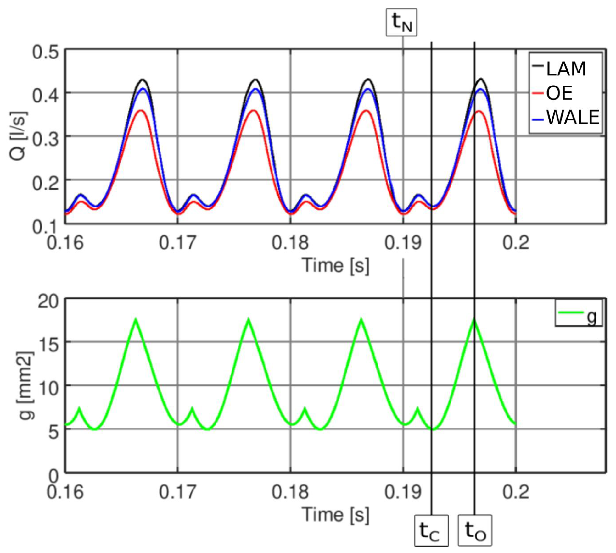
The computational mesh in the current CFD simulation is block-structured in order to capture well the boundary layer and consists of 2.1 M hexahedral elements. The mesh deforms in time due to vocal fold oscillation. The grid resolution in wall units was evaluated in three distinct time instants, corresponding to maximum opening of the vocal folds ($t_O$), maximum closure during the divergent phase ($t_N$) and maximum closure during the convergent phase ($t_C$), see

Table 2. Time instants used in the presentation of results.

Symbol	Meaning	Time [s]
$t_N$	closed divergent	0.1900
$t_C$	closed convergent	0.1927
$t_O$	open glottis	0.1963

and Figure 2. On the boundary ${\mathsf{\Gamma }}_{bVF}$ at time $t_C$ these values were evaluated: $y_{avg}^{+}=1.77$, $z_{}^{+}=14$ and $x_{}^{+}=8$.

2.4. Discretization and Numerical Solution

The Navier-Stokes equations were discretized using the collocated cell-centered Finite Volume Method. Fletcher [43] demonstrated that even-ordered derivatives in the truncation error are associated with numerical dissipation, and odd-ordered spatial derivatives are associated with the numerical dispersion in the solution. Ideally, LES simulations should use schemes with low numerical dissipation. The non-dissipative central differencing scheme (CDS), which was applied in this study, allows an accurate representation of the changing flow field [44]. The discretization of the diffusion term is split into an orthogonal and cross-diffusion term, using a procedure described in [45]. Unlike the discretization of the temporal, convective and orthogonal part of the diffusive term, the nonorthogonal correctors are treated explicitly.

The CFD simulations were run in parallel on 20 cores on a computational cluster, composed of nodes with two 10-core Intel Xeon 4114 CPUs with 96 GB RAM. In order to have sufficient resolution in the spectrum of the aeroacoustic signal, a sufficiently long simulation time t = 0.2 s, that is, 20 periods of vocal fold vibration, is needed. For such settings, one CFD simulation required 27–37 days, that is, about 15,000 core-hours of computational time.

2.5. CFD Results

The current study reports on the results of three CFD simulations using different turbulence modeling approaches, which are summarized in

Table 3. Overview of the CFD simulations.

Case	Turb. Modelling	SGS Model	Walltime
LAM	laminar	-	27 days
OE	LES	One-Equation	34 days
WALE	LES	WALE	37 days

. The laminar case “LAM” used no turbulence model. “OE” and “WALE” are LES simulations with the One-Equation and WALE SGS models, respectively. All the simulations were run for 20 periods of vocal fold oscillations, that is, $t=0.02\mathrm{s}$. The CFD simulations provide the filtered velocity and pressure fields $\overline{U}$, $\overline{p}$. For simplicity, the overbars are dropped in the following presentation.

Figure 2 shows the flow rate and glottal opening during the last four simulated cycles of vocal fold oscillation. The predicted peak flow rate in the laminar case is, for the same boundary conditions, higher than in the One-Equation and WALE SGS models by 16.76% and 5.26%, respectively. This is caused by the different values of the SGS viscosity, which add to the molecular viscosity and limit the flow rate through the glottal constriction. The laminar model does not capture the influence of small-scale turbulence, which corresponds to ${\nu }_t=0$. The WALE SGS model and the One-Equation SGS model compute with non-zero SGS viscosity, with the latter one significantly higher due to the already mentioned deficiency of the One-Equation model, which overestimates the turbulent viscosity near the vocal fold surfaces (see also Figure 6). The flow rate does not reach zero value, since the vocal folds do not fully close, corresponding physiologically to breathy phonation.

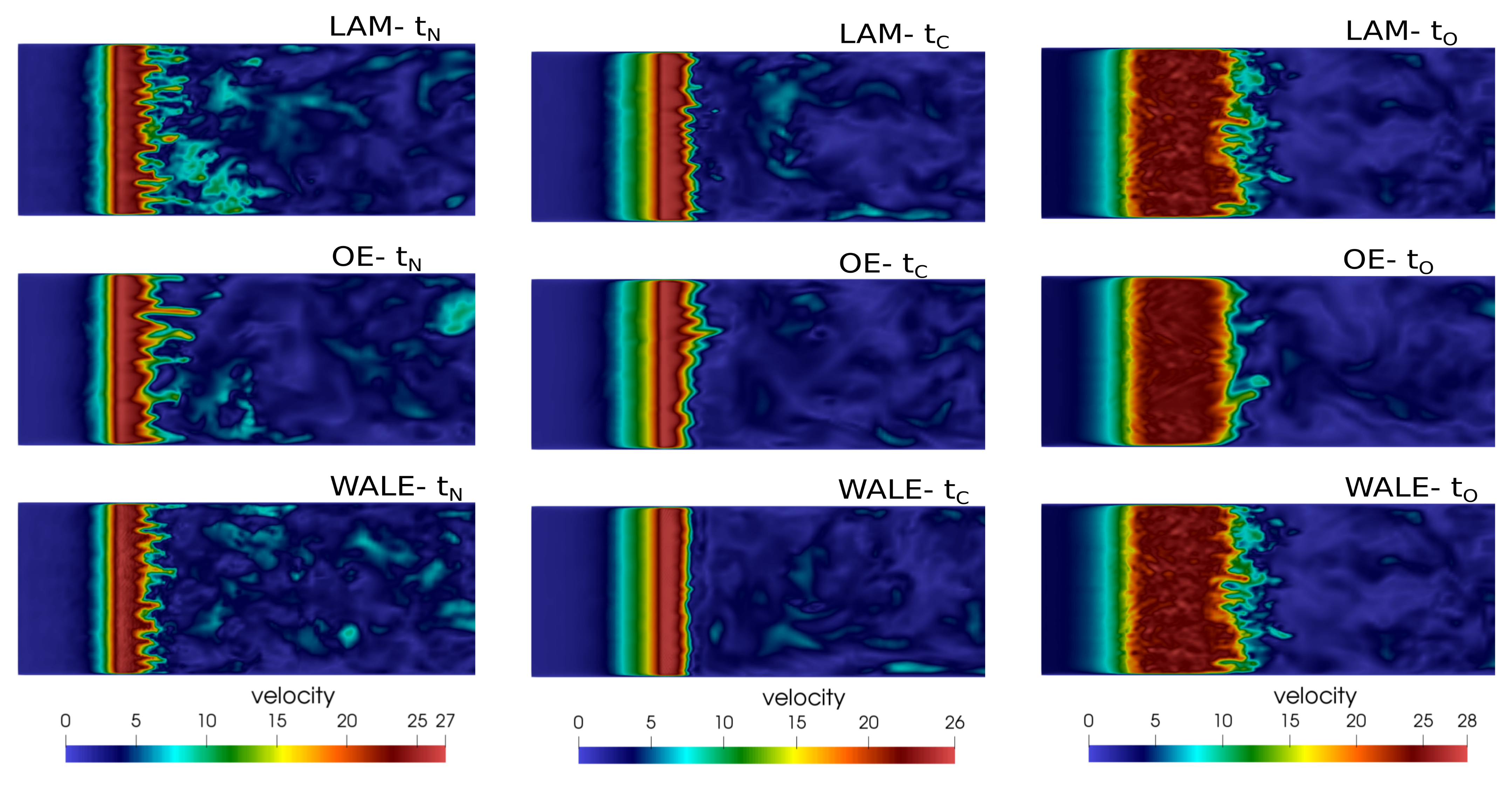
The velocity and pressure distributions along the laryngeal mid–line are plotted in Figure 3 in three distinctive times (see Table 2). The high-velocity glottal flow corresponds to a low static pressure due to the Bernoulli effect. The three simulations give almost identical results in the subglottal space, where the flow is laminar, but differ in the supraglottal volume where turbulent fluctuations are present. Figure 4, plotting the velocity fields in a sagittal (x-z) plane, shows the structure of the expanding jets during phonation.

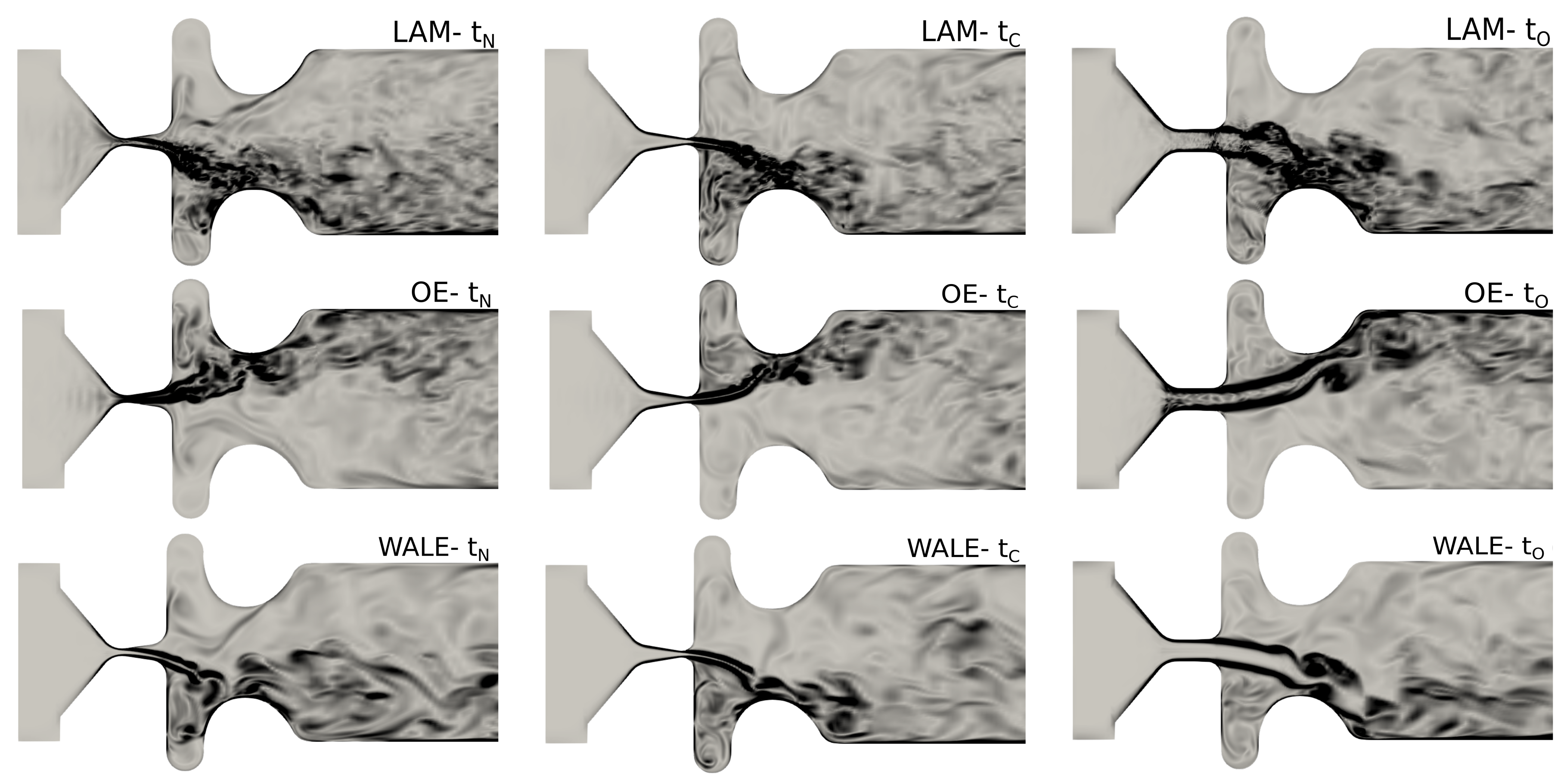
The visualizations of the vorticity fields $\mathit{\omega }=\nabla \times \mathit{U}$, which are commonly used for characterizing turbulence in cases with no entrainment rotation, are shown in mid–coronal (x-y) plane in Figure 5. They reveal the shear layers, where vortices are shed as a consequence of Kelvin-Helmholtz instability. The vortices may undergo successive instabilities, leading to a direct kinetic-energy cascade towards the small scales. The supraglottal jet deflects stochastically towards either of the ventricular folds. This behavior is not a consequence of the SGS model, it is caused by the bistability of the flow in this symmetric geometry (see e.g., [46,47]).

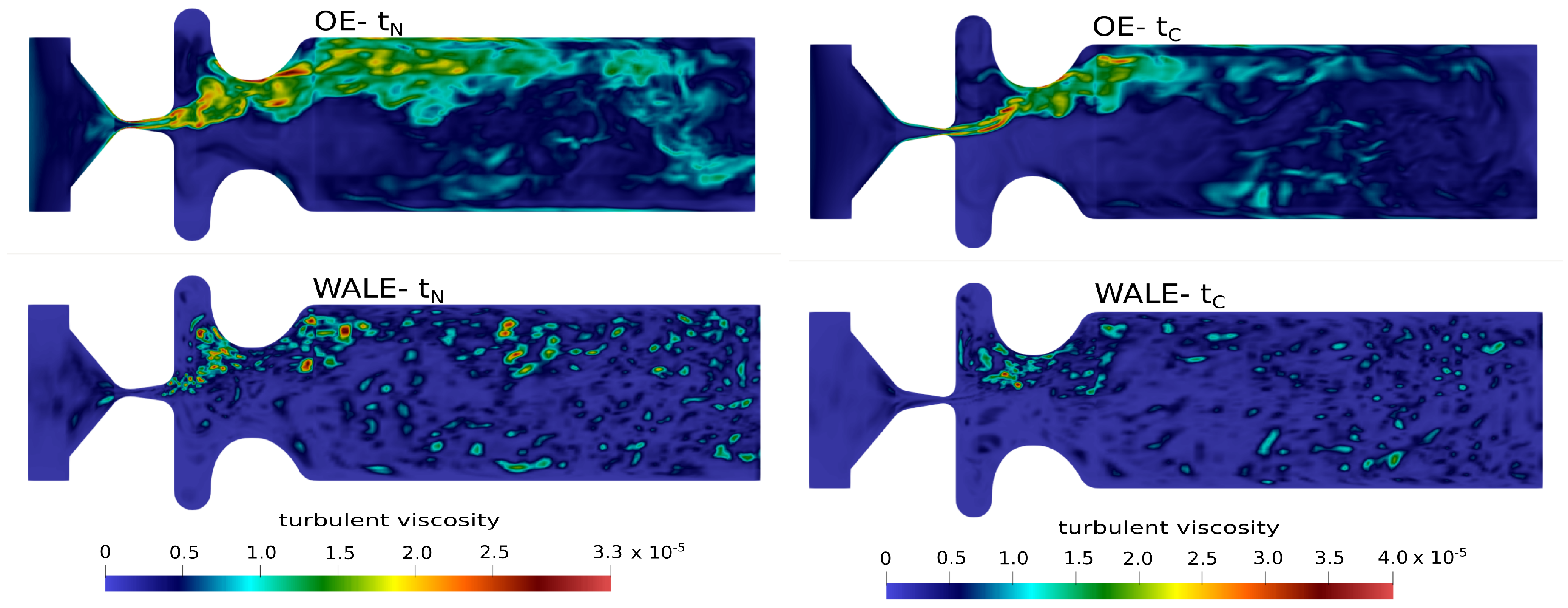
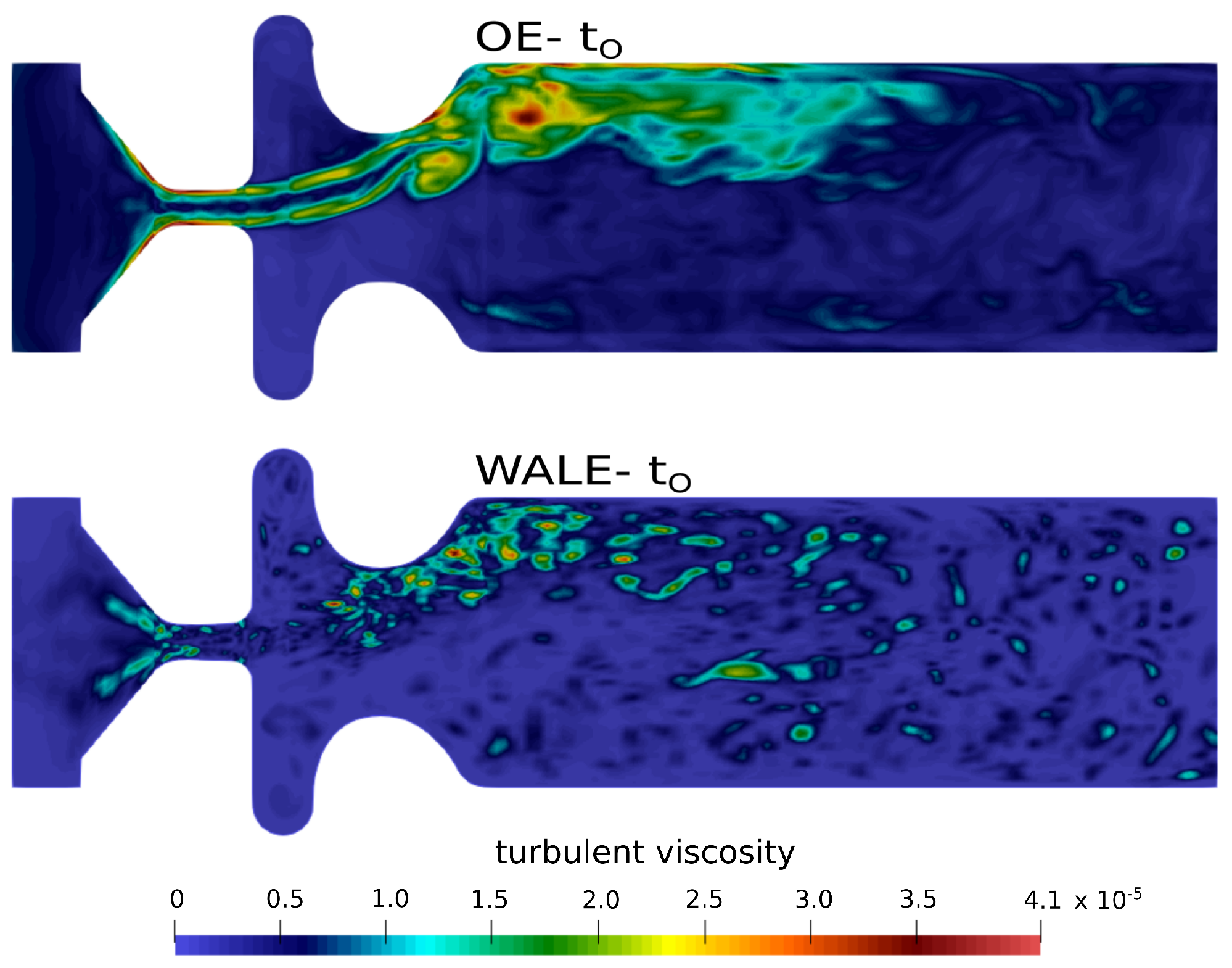
The effect of the unresolved turbulent sub-grid scales on the resolved velocity and pressure fields is carried by the turbulent SGS viscosity ${\nu }_t$ (see Equations (10) and (15)). Figure 6 clearly shows that the turbulent viscosity predicted by the One-Equation model is very high in regions of pure shear, especially within glottis. At certain phases of the vocal fold motion, ${\nu }_t$ reaches values three times higher than the molecular viscosity $\nu =1.58·{10}^{-5}{\mathrm{m}}^2{\mathrm{s}}^{-1}$. In contrast to this, the WALE SGS model predicts considerably lower values, not localized in the shear layers.

3. Computational Aeroacoustic (CAA) Model of Human Phonation

Aeroacoustics deal with flow-induced sound generation and wave propagation. The sound generation is caused by turbulent motion of fluid, periodic varying flow fields or aerodynamic forces acting on solids. The sources in the case of human phonation are commonly denoted as:

i.

A monopole source term due to the motion of vocal folds (the term is zero, when the walls are fixed and also the monopole source term at inlet is often omitted due to a non-reflecting boundary condition).

ii.

A dipole source term due to the unsteady force exerted by the surface of the vocal folds onto the fluid.

iii.

A quadrupole sound term due to the unsteady flow inside the vocal tract. See [2] for more details.

The numerical simulation of aeroacoustic effects can be realized either by using direct simulations or hybrid methods. Direct simulation is based on the compressible Navier-Stokes equations, which capture both the fluid dynamic and acoustic fluctuations. The limitation of this approach is hidden in the computational effort associated with the disparity of scales between the flow and acoustic variables (the small turbulent scales and the large acoustic wavelength during common speech), which can reach several orders of magnitude. To circumvent this problem, hybrid approaches are commonly used, where the flow field and the acoustic field are computed separately, see for example, [14,48,49]. In the current study, we used a hybrid method based on an incompressible flow computation and utilizing the perturbation ansatz to achieve the equation with which the acoustic field is computed.

3.1. Mathematical Model

The mathematical model used for aeroacoustic simulations in this study is the Perturbed Convective Wave Equation (PCWE). For understanding of the context, the idea of separation of flow variables is introduced first. In the following sections, the Acoustic Perturbation Equations (APE) will be described first. The vector-valued APEs can be further reformulated into scalar PCWE, sparing computational resources.

LES simulations provide the filtered flow variables, and so the computational aeroacoustic (CAA) simulations can work only upon the filtered velocity and pressure fields. For simplicity, the overbars from LES filtering were dropped in further presentation.

3.1.1. Acoustic Perturbation Equations (APEs)

The idea is based on using a perturbation ansatz, that is, splitting a fluid variable into an acoustic and a non-acoustic component [50]. In contrast to the Lighthill analogy, the fluctuating component is further decomposed into the incompressible and acoustic components

$$\mathit{U}={\mathit{U}}_0\left(\mathit{x}\right)+{\mathit{U}}^{\mathrm{i}c}(\mathit{x},t)+{\mathit{U}}^{\mathrm{a}}(\mathit{x},t),$$

(17)

$$p=p_0\left(\mathit{x}\right)+p^{\mathrm{i}c}(\mathit{x},t)+p^{\mathrm{a}}(\mathit{x},t),$$

(18)

$$\rho ={\rho }_0+{\rho }_1(\mathit{x},t)+{\rho }^{\mathrm{a}}(\mathit{x},t),$$

(19)

where ${\mathit{U}}_0$ is the temporal mean flow, the term ${\mathit{U}}^{\mathrm{i}c}$ represents the incompressible part of the flow velocity and ${\mathit{U}}^{\mathrm{a}}$ is the acoustic part of the flow velocity. The same decomposition is used for the pressure. The term ${\rho }_1(\mathit{x},t)$ is referred by Hardin and Pope [50] as a density correction and ensures constant entropy in the liquid, that is, ${\rho }_1=(p^{\mathrm{i}c}-\overline{p^{\mathrm{i}c}})/c_0^2$. The following assumptions are made:

• The velocity field is purely solenoidal, that is, $\nabla ·{\mathit{U}}^{\mathrm{i}c}=0$,
• The density ${\rho }_0$ is constant, that is, $\nabla {\rho }_0=0$ and $\partial {\rho }_0/\partial t=0$,
• The acoustic field is irrotational, that is, $\nabla \times {\mathit{U}}^{\mathrm{a}}=0$.

The system of equations derived from the momentum and mass conservation Equations (4) and (2), using all ansatz variables defined above, arrive at

$${\rho }_0\frac{\partial {\mathit{U}}^{\mathrm{a}}}{\partial t}+{\rho }_0({\mathit{U}}_0·\nabla ){\mathit{U}}^{\mathrm{a}}+\nabla p^{\mathrm{a}}=\mathbf{0},$$

(20)

$$\frac{\partial p^{\mathrm{a}}}{\partial t}+({\mathit{U}}_0·\nabla )p^{\mathrm{a}}+{\rho }_0{c}_0^2\nabla ·{\mathit{U}}^{\mathrm{a}}=-\frac{\partial p^{\mathrm{i}c}}{\partial t}-({\mathit{U}}_0·\nabla )p^{\mathrm{i}c}.$$

(21)

Equations (20) and (21) are called the Acoustic Perturbation Equations (for detailed derivation, we refer to [51]). The non-acoustic parts $p^{\mathrm{i}c}$ and $U_0$ are obtained from the CFD results. The time derivative of hydrodynamic pressure $\partial p^{\mathrm{i}c}/\partial t$ from the right-hand side is the major source term.

3.1.2. Perturbed Convective Wave Equation (PCWE)

Linear acoustics states the particle velocity is irrotational, $\nabla \times {\mathit{U}}^{\mathrm{a}}=0$. Hence, the form ${\mathit{U}}^{\mathrm{a}}=-\nabla {\psi }^{\mathrm{a}}$ is substituted into (20), where ${\psi }^{\mathrm{a}}$ is the scalar acoustic potential. This substitution yields

$${\rho }_0\frac{\partial (-\nabla {\psi }^{\mathrm{a}})}{\partial t}+{\rho }_0\nabla ({\mathit{U}}_0·(-\nabla {\psi }^{\mathrm{a}}))+\nabla p^{\mathrm{a}}=\mathbf{0},$$

(22)

that is

$$\nabla ({\rho }_0\frac{\partial {\psi }^{\mathrm{a}}}{\partial t}+{\rho }_0{\mathit{U}}_0·\nabla {\psi }^{\mathrm{a}}-p^{\mathrm{a}})=\mathbf{0}.$$

(23)

Thereby, it results in the relation for the acoustic pressure

$$p^{\mathrm{a}}={\rho }_0\frac{\partial {\psi }^{\mathrm{a}}}{\partial t}+{\rho }_0{\mathit{U}}_0·\nabla {\psi }^{\mathrm{a}}.$$

(24)

Substitution of (24) into (21) yields

$$\frac{\partial \left(\frac{D{\psi }^{\mathrm{a}}}{Dt}\right)}{\partial t}+{\mathit{U}}_0·\nabla \left(\frac{D{\psi }^{\mathrm{a}}}{Dt}\right)+\rho c_0^2\nabla ·{\mathit{U}}^{\mathrm{a}}=-\frac{D{p}^{\mathrm{i}c}}{Dt}.$$

(25)

Equation (25) is simplified into (26), which is a scalar-valued partial differential equation called Perturbed Convective Wave Equation [52] for the acoustic potential ${\psi }^{\mathrm{a}}$:

$$\frac{1}{c_0^2}\frac{D^2{\psi }^{\mathrm{a}}}{D{t}^2}-\nabla ·\nabla \left({\psi }^{\mathrm{a}}\right)=-\frac{1}{\rho c_0^2}\frac{D{p}^{\mathrm{i}c}}{Dt}.$$

(26)

Benefits of PCWE are the following: faster computation with a scalar unknown, lower memory requirements (compared to APE), includes convection inside the wave operator and solves for the acoustic quantity (compared to Lighthill’s analogy). The RHS in (26) is the acoustic source term.

3.2. Geometry, Mesh and Numerical Solution

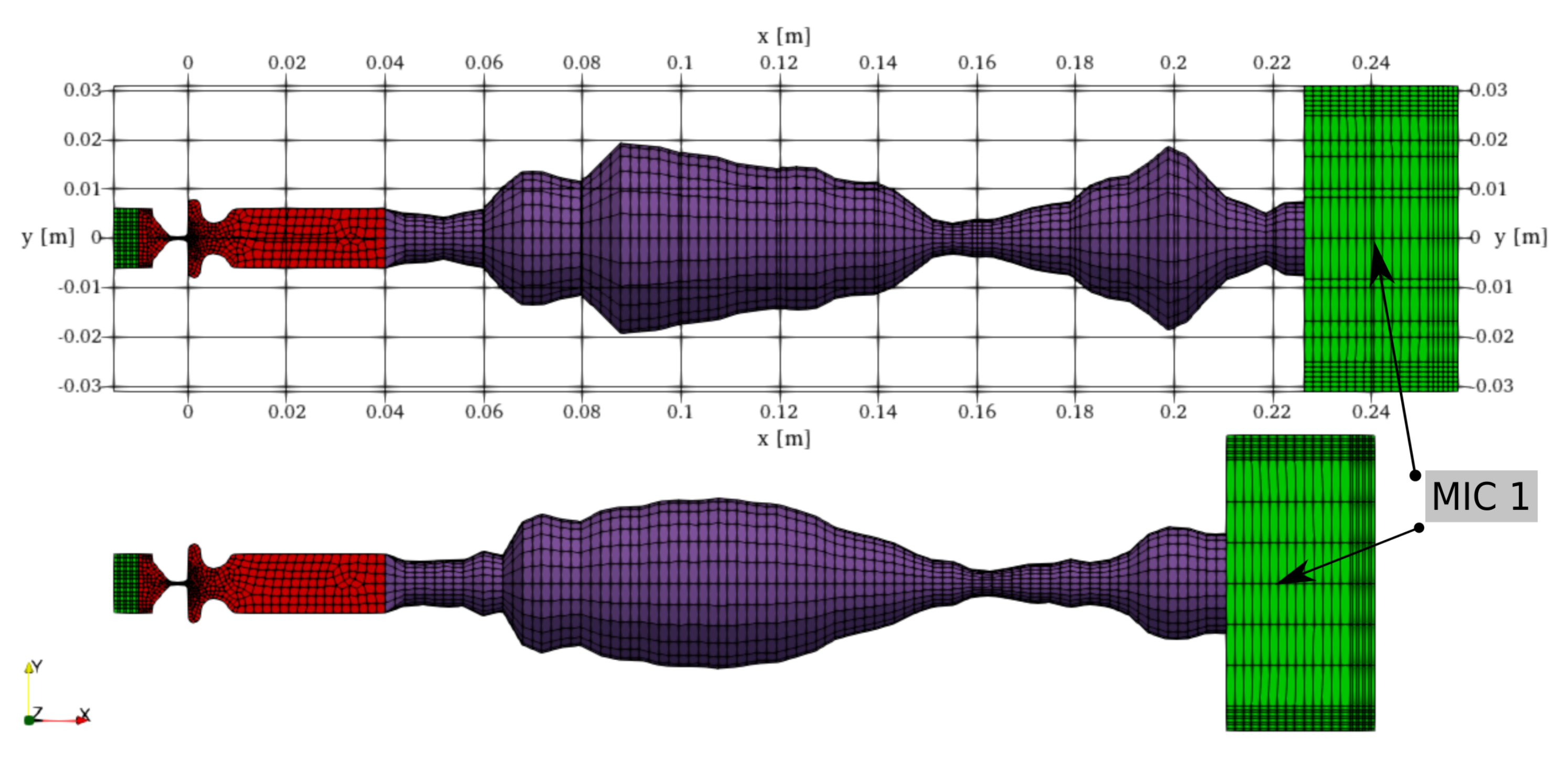
The aeroacoustic field is numerically solved by the Finite Element Method. Figure 7 illustrates the geometry and structure of the acoustic mesh. Geometries of vocal tracts for vowels [u:] and [i:] were modeled from frustums concatenated one after another. The shape of the frustums was defined according to vocal tract area functions measured by magnetic resonance imaging [53]. The vocal tracts (purple) were conformly attached to the larynx (red). The connection is formed by two hexahedral layers, with minor influence on the wave propagation. The right edge of the vocal tract is attached to the downstream radiation zone. The radiation zone is overlaid by a Perfectly Matched Layer (PML) (green) [54], with an implemented damping function to avoid reflecting waves backward. The second PML layer is inserted upstream from the inlet boundary. Microphone mic1 is located 1 cm downstream from the mouth.

The acoustic element length $\Delta l^{\mathrm{a}}$ and time step $\Delta t^{\mathrm{a}}$ for acoustics are given by estimations [51]

$$\Delta l^{\mathrm{a}}=\frac{c}{20f_{max}}=3.43\mathrm{mm},\Delta t^{\mathrm{a}}=\frac{1}{20f_{max}}=1·{10}^{-5}\mathrm{s},$$

(27)

assuming that 20 linear finite elements per one acoustic wavelength are sufficient. In our case the spatial discretization is limited by $3.43\mathrm{mm}$ and time step by $1·{10}^{-5}\mathrm{s}$ in order to resolve properly acoustic frequencies up to $f_{max}=5\mathrm{kHz}$. If the condition is not satisfied, the acoustic results are affected by high dissipation and dispersion [55]. The discretization uses hexahedral first order finite elements: 19k for vowel [u:] and 23k vowel [i:]. The acoustic material properties are defined by the density $\rho =1.11703\mathrm{kg}{\mathrm{m}}^{-3}$, the bulk modulus $K=0.1156\mathrm{MPa}$ and the speed of sound $c=343.25\mathrm{m}{\mathrm{s}}^{-1}$.

The computation of acoustic sources and simulation of the wave propagation were realized on the same computational cluster as the CFD simulations using the finite element software OpenCFS [56]. The computational times for CAA simulations are much lower than those for the CFD simulations, about 5 h on a single CPU core compared to 30 days on 20 cores. It should be noted that the conservative interpolation of the acoustic source from the CFD grid to the much coarser acoustic grid was performed also by a finite element software OpenCFS. The work of Schoder et al. [48] contains an overview of the conservative strategies, granting a reduction of simulation time.

3.3. CAA Results

Correct modeling of aeroacoustic sources is essential for the success of the hybrid aeroacoustic simulations. Therefore, the investigation of the aeroacoustic sources is presented first. In the further section, the results of six wave propagation simulations are analyzed.

3.3.1. Acoustic Sources

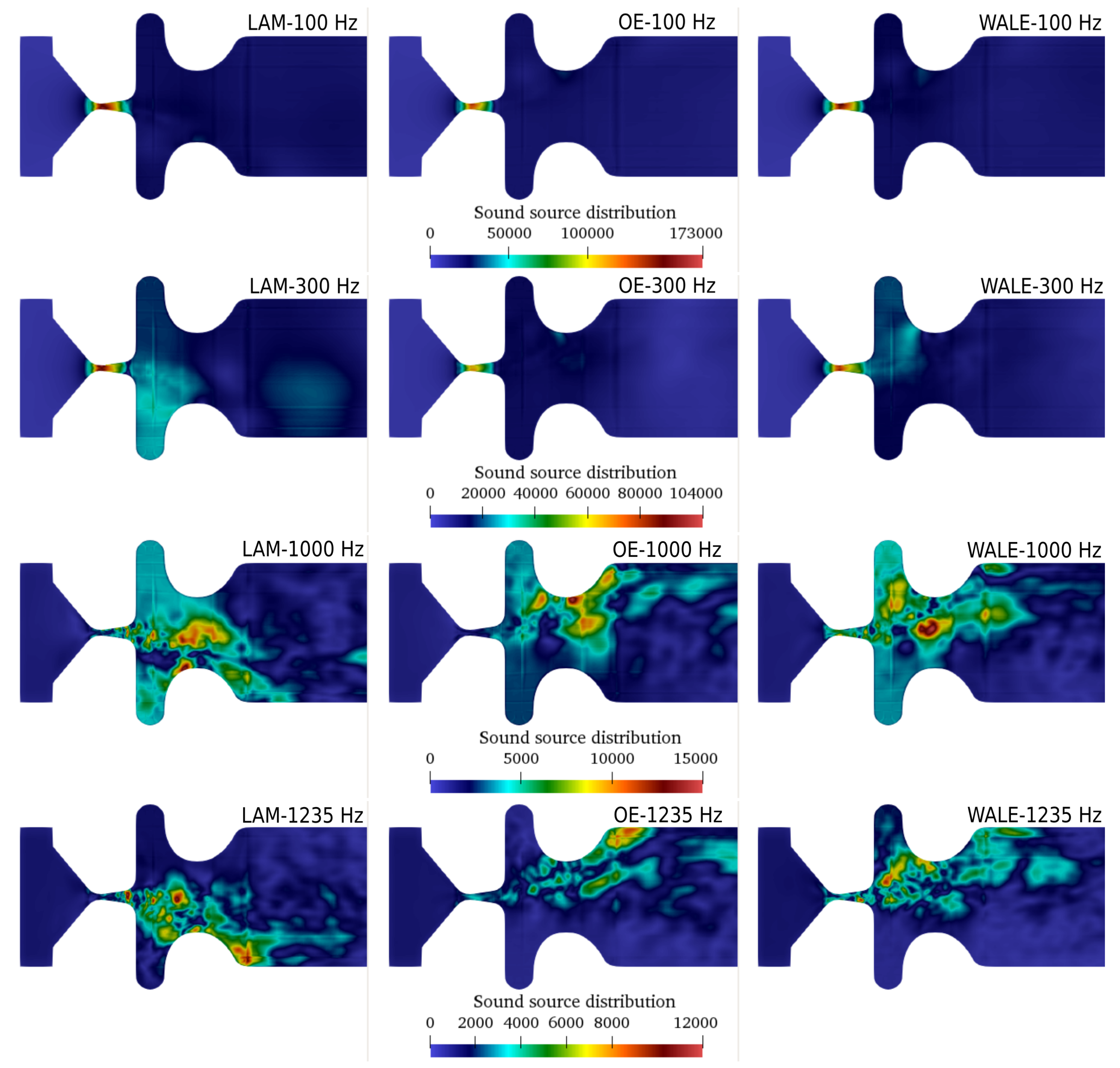
Figure 8 presents the aeroacoustic sources computed by PCWE (26) from three CFD simulations. The sources, which are a function varying in space and time, were transformed from the time domain into the frequency domain by the Fourier transform, which provides a useful insight into the spatial distribution of the sources at distinct frequencies. The first row in Figure 8 shows the aeroacoustic sources at the fundamental frequency (frequency of vibration of the vocal folds) $f_0=100\mathrm{Hz}$. The strongest sources are located inside the glottis. The laminar simulation results in slightly higher source intensities than the LES simulations. This correlates with the flow rate amplitude, which is also higher in the laminar case (see Figure 2). At the third harmonic frequency $f_2=300\mathrm{Hz}$, aeroacoustic sources are predicted also downstream of the glottis and in the supraglottal vestibule. Especially in laminar and WALE cases, disturbances induced in the shear layer of the jet are clearly visible. The third and the last row refer to a higher harmonic frequency $f_9=1000\mathrm{Hz}$ and a non-harmonic frequency $f=1235\mathrm{Hz}$. At these higher frequencies, the dominant aeroacoustic sources do not occur within glottis, but in the places, where the fast glottal jet interacts with the ventricular folds and with the slowly moving and recirculating air in the supraglottal volume.

3.3.2. Wave Propagation

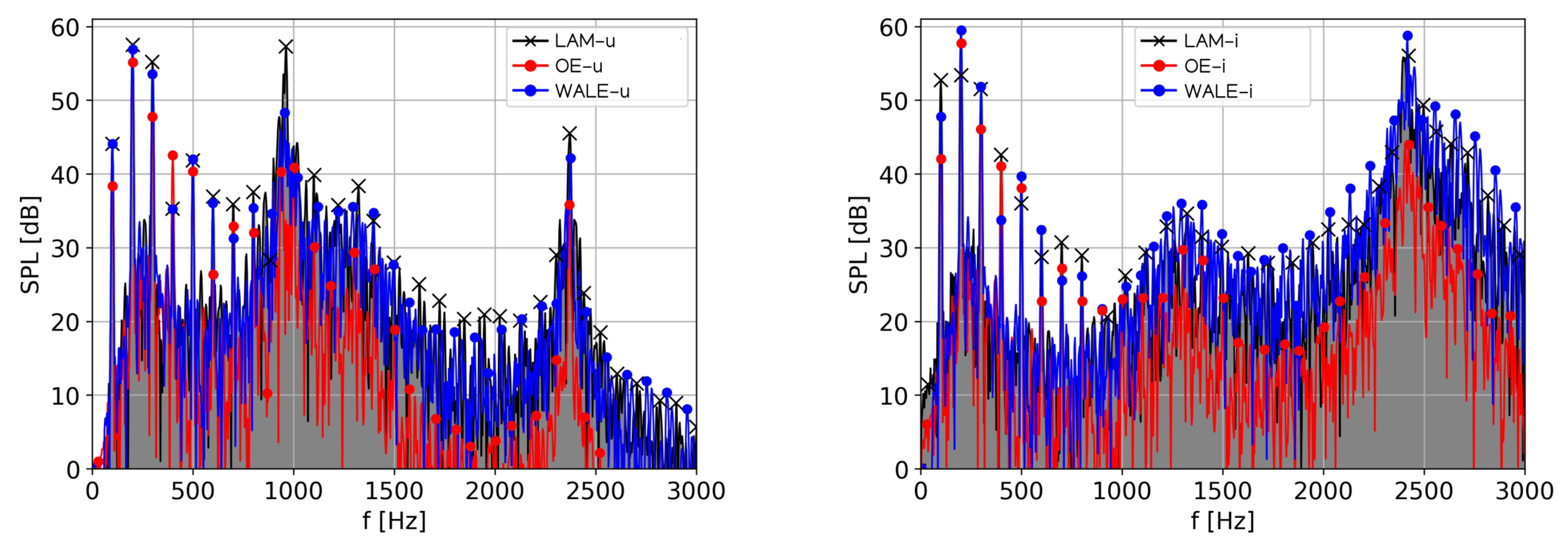
In this section, the sound pressure levels (SPL) in the frequency domain are compared. Six signals (three CFD simulations and two types of vocal tract models) were used for spectral analysis, with the frequency resolution $\Delta f=5\mathrm{Hz}$ and the Hanning windowing. The spectra of the acoustic pressure evaluated at the acoustic probe mic1 (see Figure 7) are depicted in Figure 9 for two types of vocal tracts. The vowel [u:] is characterized by formant frequencies $f_{F1}^{u:}=270\mathrm{Hz}$, $f_{F2}^{u:}=1000\mathrm{Hz}$ and $f_{F3}^{u:}=2484\mathrm{Hz}$ [53]. The tolerable bandwidths are defined as $B_{F1}=\pm 100\mathrm{Hz}$ and $B_{F2,F3}=\pm 200\mathrm{Hz}$. The usage of SGS models does not modify positions of formant frequencies, but it modifies considerably the SPLs ($L_F^{u:}$ and $L_F^{i:}$), see details in

Table 4. Sound pressure levels [dB] at probe MIC 1 for aeroacoustic simulations (vowel u: and i:), based on CFD simulations with the laminar, One-Equation and Wall-Adapting Local Eddy-viscosity (WALE) sub-grid scale (SGS) models. Values at $f_o=100\mathrm{Hz}$, $f_1=200\mathrm{Hz}$, $f_2=300\mathrm{Hz}$, non-harmonic frequency $1235\mathrm{Hz}$ and formant frequencies.

Case	${\mathit{L}}_{{\mathit{f}}_{\mathit{o}}}$	${\mathit{L}}_{{\mathit{f}}_1}$	${\mathit{L}}_{{\mathit{f}}_2}$	${\mathit{L}}_{1235}$	${\mathit{L}}_{\mathit{F}1}^{\mathit{u}:}$	${\mathit{L}}_{\mathit{F}2}^{\mathit{u}:}$	${\mathit{L}}_{\mathit{F}3}^{\mathit{u}:}$
LAM-u	44.05	57.48	55.20	33.12	34.25	57.31	45.49
OE-u	38.34	55.13	47.79	15.33	28.94	40.88	35.76
WALE-u	44.06	56.86	53.52	20.03	33.42	48.29	42.15
Case	${\mathit{L}}_{{\mathit{f}}_{\mathit{o}}}$	${\mathit{L}}_{{\mathit{f}}_1}$	${\mathit{L}}_{{\mathit{f}}_2}$	${\mathit{L}}_{1235}$	${\mathit{L}}_{\mathit{F}1}^{\mathit{i}:}$	${\mathit{L}}_{\mathit{F}2}^{\mathit{i}:}$	${\mathit{L}}_{\mathit{F}3}^{\mathit{i}:}$
LAM-i	52.68	53.31	51.52	28.99	32.46	34.62	56.02
OE-i	42.07	57.76	46.08	15.24	28.49	29.70	43.95
WALE-i	47.69	59.45	51.88	19.86	34.13	35.96	58.77

. The intensity of the third formant $L_{F3}^u$ computed using the WALE model reached 42 dB, compared to 36 dB in the aeroacoustic simulation based on the One-Equation SGS model. All formant frequencies computed by the One-Equation SGS model are weaker compared to the WALE SGS model and the laminar model by 5–7 dB and 6–17 dB, respectively.

In the case of the vowel [i:], the formant frequencies reported in the literature are $f_{F1}^{i:}$ = 289 Hz, $f_{F2}^{i:}$ = 987 Hz, $f_{F3}^{i:}$ = 2299 Hz. Similar to the previous case, the WALE SGS model has computed the $L_{F2}^{i:}$ and $L_{F3}^{i:}$ stronger compared to the One-Equation SGS model by 6 dB and 15 dB, respectively.

Figure 9 also shows that the simulations using the WALE SGS model for both vowels result in significantly enforced higher harmonic frequencies $n{f}_o$ compared to the One-Equation SGS model for both vowels. In the case of vowel [u:], the harmonic frequencies above 1000 Hz for the WALE SGS model are even stronger than the aeroacoustic output based on the laminar CFD simulation.

4. Discussion and Conclusions

Large Eddy Simulations of subsonic incompressible flow in a model of human larynx were realized. The effect of the SGS turbulence model on the flow field, namely the flow rate, velocity, pressure and vorticity was analyzed in three variants—the laminar (no SGS), One-Equation and WALE SGS model. Compared to the classical Smagorinsky algebraic SGS model, the One-Equation SGS model has two prominent features—it is more suitable for high Reynolds number flows and avoids the inaccurate assumption of local balance between SGS energy production and dissipation [57]. However, similar to the Smagorinsky model, the One-Equation model is known to over predict the turbulent viscosity in regions where shear is dominant, that is, in the boundary layer adjacent to the vocal folds and in the shear layers of the glottal jet. The WALE SGS model, on the contrary, produces zero eddy viscosity in cases of pure shear flow, and recovers the proper $y^3$ near-wall scaling for the eddy (turbulent) viscosity without requiring a dynamic procedure. Moreover, Nicoud and Ducros [30] showed that it can handle laminar-turbulent transition, which makes it attractive for complex geometries and specifically for glottal flow simulations.

In the results of the CFD simulations, the waveforms of the flow rate show that the peak flow rate simulated by the One-Equation and WALE SGS models is lower than in the laminar case by 16.76% and 5.26%, respectively. It is necessary to note that these values are obtained for airflow driven by constant transglottal pressure. Other studies commonly prescribe a less realistic constant inlet velocity condition, where this effect cannot be observed. In our simulations, the differences in the peak flow rate are clearly induced by the SGS model, which acts through the turbulent SGS viscosity adding to the molecular viscosity of air and helps to block the airflow in the narrowest constriction between the vocal folds. The results prove that the WALE model predicts considerably lower, and presumably more realistic, values, not localized in the shear layers.

Due to the disparity of scales between the flow structures and acoustic wavelengths, a hybrid aeroacoustic approach based on the perturbed compressible wave equations was used. The flow results computed by the Finite Volume method were used to evaluate the aeroacoustic sources. These were interpolated from the fine grid covering the larynx to the coarse grid of the larynx and vocal tract, where the acoustic variables were computed by the finite element method.

The visualization of the aeroacoustic sources in the frequency domain shows that the laminar and WALE models predict slightly stronger aeroacoustic sources compared to the One-Equation model. Sound sources at the fundamental frequency $f_0$ are located primarily in the glottis. At higher harmonic frequencies, the sources are distributed also in the supraglottal vestibule and further downstream of the glottis, especially in the shear layer of the jet and in places, where the fast glottal jet interacts with the ventricular folds and with the slowly recirculating air in the supraglottal spaces.

The acoustic spectra of the sound evaluated 1 cm from the lips show important differences between the simulations based on the laminar CFD data, and LES simulations with the One-Equation and WALE SGS models. The sound pressure levels from the WALE simulation are significantly higher than those from the One-Equation model, especially at frequencies above $1000\mathrm{Hz}$, where the difference reaches up to $15\mathrm{dB}$. In the case of the vowel [i:], the SPL predictions based on the WALE model exceed even those from the laminar model. This can be partly explained by the fact that the CFD simulations using the One-Equation model result in lower flow rates and pressure fluctuations. However, at lower frequencies, the trend in the acoustic spectra is more ambiguous: the differences between the three models are less significant and, for example, at the third harmonic, the WALE model gives even lower SPLs than the One-Equation model. Thus, the differences cannot be attributed only to the amplitude of the underlying fluid flow pulsation. It may be concluded that the WALE SGS model performs better not only in the CFD simulation, where we know from theory that it handles more correctly the boundary and shear layers, but that its effect is also beneficial for the subsequent aeroacoustic simulations of the human voice, where it promotes the higher harmonic content in the acoustic spectrum.

References

- Titze, I.R. Principles of Voice Production; Prentice Hall: Englewood Cliffs, NJ, USA, 1994. [Google Scholar]
- Zhao, W.; Zhang, C.; Frankel, S.H.; Mongeau, L. Computational aeroacoustics of phonation, Part I: Computational methods and sound generation mechanisms. J. Acoust. Soc. Am. 2002, 112, 2134–2146. [Google Scholar] [CrossRef]
- Zhang, Z.; Mongeau, L.; Frankel, S.H. Experimental verification of the quasi-steady approximation for aerodynamic sound generation by pulsating jets in tubes. J. Acoust. Soc. Am. 2002, 112, 1652–1663. [Google Scholar] [CrossRef]
- Dollinger, M.; Kobler, J.; Berry, D.A.; Mehta, D.; Luegmair, G.; Bohr, C. Experiments on Analysing Voice Production: Excised (Human, Animal) and In Vivo (Animal) Approaches. Curr. Bioinform. 2011, 6, 286–304. [Google Scholar] [CrossRef] [PubMed] [Green Version]
- Kniesburges, S.; Thomson, S.L.; Barney, A.; Triep, M.; Šidlof, P.; Horáček, J.; Brücker, C.; Becker, S. In vitro experimental investigation of voice production. Curr. Bioinform. 2011, 6, 305–322. [Google Scholar] [CrossRef] [PubMed] [Green Version]
- Sadeghi, H.; Döllinger, M.; Kaltenbacher, M.; Kniesburges, S. Aerodynamic impact of the ventricular folds in computational larynx models. J. Acoust. Soc. Am. 2019, 145, 2376–2387. [Google Scholar] [CrossRef]
- Sadeghi, H.; Kniesburges, S.; Falk, S.; Kaltenbacher, M.; Schützenberger, A.; Döllinger, M. Towards a Clinically Applicable Computational Larynx Model. Appl. Sci. 2019, 9, 2288. [Google Scholar] [CrossRef] [Green Version]
- Alipour, F.; Scherer, R.C. Pulsatile airflow during phonation: An excised larynx model. J. Acoust. Soc. Am. 1995, 97, 1241–1248. [Google Scholar] [CrossRef]
- Oren, L.; Khosla, S.; Murugappan, S.; King, R.; Gutmark, E. Role of Subglottal Shape in Turbulence Reduction. Ann. Otol. Rhinol. Laryngol. 2009, 118, 232–240. [Google Scholar] [CrossRef] [PubMed]
- Alipour, F.; Scherer, R.C. Characterizing glottal jet turbulence. J. Acoust. Soc. Am. 2006, 119, 1063–1073. [Google Scholar] [CrossRef]
- Zhang, Z. Mechanics of human voice production and control. J. Acoust. Soc. Am. 2016, 140, 2614–2635. [Google Scholar] [CrossRef] [PubMed] [Green Version]
- de Oliviera-Rosa, M.; Pereira, J.; Grellet, M.; Alwan, A. A contribution to simulating a three-dimensional larynx model using the finite element method. J. Acoust. Soc. Am. 2003, 114, 2893–2905. [Google Scholar] [CrossRef] [Green Version]
- Alipour, F.; Scherer, R.C. Flow separation in a computational oscillating vocal fold model. J. Acoust. Soc. Am. 2004, 116, 1710–1719. [Google Scholar] [CrossRef] [PubMed]
- Bae, Y.; Moon, Y.J. Computation of phonation aeroacoustics by an INS/PCE splitting method. Comput. Fluids 2008, 37, 1332–1343. [Google Scholar] [CrossRef]
- Larsson, M.; Müller, B. Numerical simulation of confined pulsating jets in human phonation. Comput. Fluids 2009, 38, 1375–1383. [Google Scholar] [CrossRef] [Green Version]
- Link, G.; Kaltenbacher, M.; Breuer, M.; Döllinger, M. A 2D finite-element scheme for fluid–solid–acoustic interactions and its application to human phonation. Comput. Methods Appl. Mech. Eng. 2009, 198, 3321–3334. [Google Scholar] [CrossRef]
- Thomson, S. Investigating coupled flow-structure-acoustic interactions of human vocal fold flow-induced vibration. J. Acoust. Soc. Am. 2015, 138, 1776. [Google Scholar] [CrossRef]
- Šidlof, P.; Zörner, S.; Hüppe, A. A hybrid approach to computational aeroacoustics of human voice production. Biomech. Model. Mechanobiol. 2015, 14, 473–488. [Google Scholar] [CrossRef]
- Jiang, W.; Zheng, X.; Xue, Q. Computational Modeling of Fluid–Structure–Acoustics Interaction during Voice Production. Front. Bioeng. Biotechnol. 2017, 5, 7. [Google Scholar] [CrossRef] [Green Version]
- Sváček, P.; Horáček, J. Finite element approximation of flow induced vibrations of human vocal folds model: Effects of inflow boundary conditions and the length of subglottal and supraglottal channel on phonation onset. Appl. Math. Comput. 2018, 319, 178–194. [Google Scholar] [CrossRef]
- Suh, J.; Frankel, S. Numerical simulation of turbulence transition and sound radiation for flow through a rigid glottal model. J. Acoust. Soc. Am. 2007, 121, 3728–3739. [Google Scholar] [CrossRef]
- Mihaescu, M.; Khosla, S.M.; Murugappan, S.; Gutmark, E.J. Unsteady laryngeal airflow simulations of the intra-glottal vortical structures. J. Acoust. Soc. Am. 2010, 127, 435–444. [Google Scholar] [CrossRef] [PubMed]
- Mihaescu, M.; Mylavarapu, G.; Gutmark, E.J.; Powell, N.B. Large Eddy Simulation of the pharyngeal airflow associated with Obstructive Sleep Apnea Syndrome at pre and post-surgical treatment. J. Biomech. 2011, 44, 2221–2228. [Google Scholar] [CrossRef]
- Schwarze, R.; Mattheus, W.; Klostermann, J.; Brücker, C. Starting jet flows in a three-dimensional channel with larynx-shaped constriction. Comput. Fluids 2011, 48, 68–83. [Google Scholar] [CrossRef] [Green Version]
- de Luzan, C.F.; Chen, J.; Mihaescu, M.; Khosla, S.M.; Gutmark, E. Computational study of false vocal folds effects on unsteady airflows through static models of the human larynx. J. Biomech. 2015, 48, 1248–1257. [Google Scholar] [CrossRef] [Green Version]
- Sadeghi, H.; Kniesburges, S.; Kaltenbacher, M.; Schützenberger, A.; Döllinger, M. Computational Models of Laryngeal Aerodynamics: Potentials and Numerical Costs. J. Voice 2018. [Google Scholar] [CrossRef] [PubMed]
- Schickhofer, L.; Malinen, J.; Mihaescu, M. Compressible flow simulations of voiced speech using rigid vocal tract geometries acquired by MRI. J. Acoust. Soc. Am. 2019, 145, 2049–2061. [Google Scholar] [CrossRef]
- Zörner, S.; Šidlof, P.; Hüppe, A.; Kaltenbacher, M. Flow and Acoustic Effects in the Larynx for Varying Geometries. Acta Acust. United Acust. 2016, 102, 257–267. [Google Scholar] [CrossRef]
- Yoshizawa, A.; Horiuti, K. A statistically-derived subgrid-scale kinetic energy model for the large-eddy simulation of turbulent flows. J. Phys. Soc. Jpn. 1985, 54, 2834–2839. [Google Scholar] [CrossRef]
- Nicoud, F.; Ducros, F. Subgrid-scale stress modelling based on the square of the velocity gradient tensor. Flow Turbul. Combust. 1999, 62, 183–200. [Google Scholar] [CrossRef]
- Lesieur, M.; Métais, O.; Comte, P. Large-Eddy Simulations of Turbulence; Cambridge University Press: Cambridge, UK, 2005. [Google Scholar]
- Versteeg, H.K.; Malalasekera, W. An Introduction to Computational Fluid Dynamics: The Finite Volume Method; Pearson Education: London, UK, 2007. [Google Scholar]
- Ferziger, H. Direct and large eddy simulation of turbulence. Numer. Methods Fluid Mech. 1998, 16, 53–73. [Google Scholar]
- Clark, A.; Ferziger, H.; Reynolds, C. Evaluation of subgrid-scale models using an accurately simulated turbulent flow. J. Fluid Mech. 1979, 91, 1–16. [Google Scholar] [CrossRef]
- Leonard, A. Energy cascade in large-eddy simulations of turbulent fluid flows. In Advances in Geophysics; Elsevier: Amsterdam, The Netherlands, 1975; Volume 18, pp. 237–248. [Google Scholar]
- Smagorinsky, J. General circulation experiments with the primitive equations: I. The basic experiment. Mon. Weather Rev. 1963, 91, 99–164. [Google Scholar] [CrossRef]
- Šidlof, P. Large eddy simulation of airflow in human vocal folds. In Topical Problems of Fluid Mechanics 2015; Institute of Thermomechanics: Prague, Czech Republic, 2015; pp. 187–196. [Google Scholar]
- Scherer, R.; Shinwari, D.; De Witt, J.; Zhang, C.; Kucinschi, R.; Afjeh, A. Intraglottal pressure profiles for a symmetric and oblique glottis with a divergence angle of 10 degrees. J. Acoust. Soc. Am. 2001, 109, 1616–1630. [Google Scholar] [CrossRef]
- Agarwal, M.; Scherer, R.; Hollien, H. The false vocal folds: Shape and size in frontal view during phonation based on laminagraphic tracings. J. Voice 2003, 17, 97–113. [Google Scholar] [CrossRef]
- Pope, S.B. Turbulent Flows; Cambridge University Press: Cambridge, UK, 2000. [Google Scholar] [CrossRef]
- Georgiadis, N.J.; Rizzetta, D.P.; Fureby, C. Large-eddy simulation: Current capabilities, recommended practices, and future research. AIAA J. 2010, 48, 1772–1784. [Google Scholar] [CrossRef]
- Jiang, X.; Lai, C.H. Numerical Techniques for Direct and Large-Eddy Simulations; CRC Press: Boca Raton, FL, USA; Taylor & Francis Group: Abingdon, UK, 2009. [Google Scholar]
- Fletcher, C.A. Fluid Dynamics: The Governing Equations. In Computational Techniques for Fluid Dynamics 2; Springer: Berlin/Heidelberg, Germany, 1991; pp. 1–46. [Google Scholar]
- Launchbury, D.R. Unsteady Turbulent Flow Modelling and Applications; Springer: Berlin/Heidelberg, Germany, 2016. [Google Scholar]
- Jasak, H. Error Analysis and Estimation for the Finite Volume Method with Applications to Fluid Flows. Ph.D. Thesis, Imperial College of Science, Technology and Medicine, London, UK, 1996. [Google Scholar]
- Erath, B.; Plesniak, M. An investigation of asymmetric flow features in a scaled-up driven model of the human vocal folds. Exp. Fluids 2010, 49, 131–146. [Google Scholar] [CrossRef]
- Lodermeyer, A.; Becker, S.; Döllinger, M.; Kniesburges, S. Phase-locked flow field analysis in a synthetic human larynx model. Exp. Fluids 2015, 56. [Google Scholar] [CrossRef]
- Schoder, S.; Weitz, M.; Maurerlehner, P.; Hauser, A.; Falk, S.; Kniesburges, S.; Döllinger, M.; Kaltenbacher, M. Hybrid aeroacoustic approach for the efficient numerical simulation of human phonation. J. Acoust. Soc. Am. 2020, 147, 1179–1194. [Google Scholar] [CrossRef] [PubMed]
- Valášek, J.; Kaltenbacher, M.; Sváček, P. On the application of acoustic analogies in the numerical simulation of human phonation process. Flow Turbul. Combust. 2018, 102, 129–143. [Google Scholar] [CrossRef]
- Hardin, J.C.; Pope, D.S. An acoustic/viscous splitting technique for computational aeroacoustics. Theor. Comput. Fluid Dyn. 1994, 6, 323–340. [Google Scholar] [CrossRef]
- Hüppe, A. Spectral Finite Elements for Acoustic Field Computation (Measurement-, Actuator-, and Simulation-Technology). Ph.D. Thesis, Shaker Verlag GmbH, Düren, Germany, 2014. [Google Scholar] [CrossRef]
- Hüppe, A.; Grabinger, J.; Kaltenbacher, M.; Reppenhagen, A.; Dutzler, G.; Kühnel, W. A non-conforming finite element method for computational aeroacoustics in rotating systems. In Proceedings of the 20th AIAA/CEAS Aeroacoustics Conference, Atlanta, GA, USA, 16–20 June 2014; p. 2739. [Google Scholar]
- Story, B.H.; Titze, I.R.; Hoffman, E.A. Vocal tract area functions from magnetic resonance imaging. J. Acoust. Soc. Am. 1996, 100, 537–554. [Google Scholar] [CrossRef] [PubMed]
- Kaltenbacher, B.; Kaltenbacher, M.; Sim, I. A modified and stable version of a perfectly matched layer technique for the 3-d second order wave equation in time domain with an application to aeroacoustics. J. Comput. Phys. 2013, 235, 407–422. [Google Scholar] [CrossRef] [PubMed] [Green Version]
- Kaltenbacher, M. Numerical Simulation of Mechatronic Sensors and Actuators: Finite Elements for Computational Multiphysics; Springer: Berlin, Germany, 2015. [Google Scholar]
- Kaltenbacher, M. OpenCFS—Open Source Finite Element Software for Multi-Physical Simulation. Available online: https://www.opencfs.org (accessed on 21 February 2021).
- Huang, S.; Li, Q. A new dynamic one-equation subgrid-scale model for large eddy simulations. Int. J. Numer. Methods Eng. 2010, 81, 835–865. [Google Scholar] [CrossRef]
Figure 1.
CFD computational domain in mid–coronal section and details of the CFD mesh near the vocal and ventricular folds. The z-normal boundaries are denoted and .
Figure 2.
Flow rates during four oscillation cycles and glottal surface.
Figure 3.
Velocity magnitude (left) and pressure distribution (right) along the glottal mid–line in three time instants (top), (middle) and (bottom). Gray background denotes the region of the moving vocal folds.
Figure 4.
Velocity fields [] in mid–sagittal plane in three time instants.
Figure 5.
Vorticity fields in mid–coronal plane in range (0, 30,000) [].
Figure 6.
Turbulent viscosity [] in mid–coronal plane.
Figure 7.
Geometry, mesh and probe location for computational aeroacoustic (CAA) simulations—vocal tracts [u:] (top) and [i:] (bottom). Red—larynx, purple—vocal tract, green—PML.
Figure 8.
Spatial distribution of sound sources [] in mid–coronal plane at four frequencies (as a result of Fast Fourier Transform).
Figure 9.
Acoustic sound spectra from the numerical simulation of vocalization of [u:] (left) and [i:] (right) at monitoring point “MIC 1”.