Article

Efficient Operative Cost Reduction in Distribution Grids Considering the Optimal Placement and Sizing of D-STATCOMs Using a Discrete-Continuous VSA

by
Oscar Danilo Montoya
1,2,*,
Walter Gil-González
3 and
Jesus C. Hernández
4
1
Facultad de Ingeniería, Universidad Distrital Francisco José de Caldas, Bogotá D.C. 11021, Colombia
2
Laboratorio Inteligente de Energía, Universidad Tecnológica de Bolívar, Cartagena 131001, Colombia
3
Grupo GIIEN, Facultad de Ingeniería, Institución Universitaria Pascual Bravo, Campus Robledo, Medellín 050036, Colombia
4
Department of Electrical Engineering, Campus Lagunillas s/n, University of Jaén, Edificio A3, 23071 Jaén, Spain
*
Author to whom correspondence should be addressed.
Submission received: 19 January 2021 / Revised: 4 February 2021 / Accepted: 5 February 2021 / Published: 2 March 2021
(This article belongs to the Special Issue Power Electronics in Power Networks)

Abstract

:
The problem of reactive power compensation in electric distribution networks is addressed in this research paper from the point of view of the combinatorial optimization using a new discrete-continuous version of the vortex search algorithm (DCVSA). To explore and exploit the solution space, a discrete-continuous codification of the solution vector is proposed, where the discrete part determines the nodes where the distribution static compensator (D-STATCOM) will be installed, and the continuous part of the codification determines the optimal sizes of the D-STATCOMs. The main advantage of such codification is that the mixed-integer nonlinear programming model (MINLP) that represents the problem of optimal placement and sizing of the D-STATCOMs in distribution networks only requires a classical power flow method to evaluate the objective function, which implies that it can be implemented in any programming language. The objective function is the total costs of the grid power losses and the annualized investment costs in D-STATCOMs. In addition, to include the impact of the daily load variations, the active and reactive power demand curves are included in the optimization model. Numerical results in two radial test feeders with 33 and 69 buses demonstrate that the proposed DCVSA can solve the MINLP model with best results when compared with the MINLP solvers available in the GAMS software. All the simulations are implemented in MATLAB software using its programming environment.

1. Introduction

Around the world, electric distribution networks are the channels through which electricity is supplied to millions of end-users at medium- and low-voltage levels [1]. These grids are constantly submitted to increments in the load consumption each year. Therefore, these networks must be prepared to receive new users and guarantee the quality, reliability and security of the public service [2,3]. Due to the operational voltages, i.e., typically between 10 kV and 15 kV for the Colombian medium-voltage distribution grids, these electrical networks experience higher energy losses as compared to the transmission and sub-transmission systems [4]. In the Colombian context the power system has energy losses of about 1.5% to 2.0% in terms of the total energy transmitted. In the medium-voltage grids energy losses can vary from 5% to 18%, and the lowest losses are found in networks of the grid operators who invested to improve the quality of their grids [5]. The difference between energy losses is principally caused by the radial topology which is typically adopted while building the distribution networks to minimize investment costs. This topology is in contrast with the strong meshed structures that are found in power systems. The main problem with the radial topology of the electric distribution grids is the high percentages of energy losses caused by the electricity distribution tasks [6]. To reduce the energy losses in the distribution service, the Utilities can use various methodologies, such as (i) grid reconfiguration [7], (ii) optimal location of shunt capacitors [8] and (iii) optimal location of dispersed power generation plants [9]. These approaches can achieve different levels of reduction of energy losses. Of these methodologies, distributed generation is the best option for energy loss reduction. However, its initial installation costs can be very high as compared to the reconfiguration and shunt capacitor approaches. However, the main problem of the capacitor banks is that they inject only in fixed steps of reactive power (discrete nature of the capacitive compensation with shunt capacitors), while the daily active and reactive power demands along the electric distribution grids are highly variables and continuous [10]. Recognizing the power saving that can be achieved with reactive power compensation with shunt devices, in recent decades, compensators based on power electronics have gained taken importance in distribution levels due to their versatility and capacity to vary the reactive power injections as a function of the demand behavior. These devices are the distribution static compensators (D-STATCOMs) [11], which have, among others, such advantages as: (i) high reliability, (ii) low operative costs, and (iii) long useful life (typically 5 to 15 years).
The literature on this specific topic has reported several approaches regarding the use of D-STATCOMs for dynamic reactive power compensation at medium-voltage levels. Some of these approaches are presented below. The authors of [11] presented the complete of determining the optimal placement and sizing of D-STATCOMs using analytical and heuristic optimization methods. Also, they presented some objective classical functions used for improving the grid performance, such as voltage stability and power loss indices. In [6] the authors proposed a multi-objective particle swarm optimizer to locate and size D-STATCOMs considering the simultaneous reconfiguration of the electrical network. As objective functions are considered the minimizing the active power losses, the voltage stability index and the loadability factor of the distribution lines, the main characteristic of this approach is that the optimization process is made only during the peak load condition, which is not considered a proper scenario due to possible over-sizing of the compensator devices, since the active and reactive power consumptions are variable inputs. The authors in [12] presented a heuristic cost-based approach to evaluate the impact of the optimal placement and sizing of D-STATCOMs in isolated power systems for automatic voltage support. However, the model considers the unique nodal representation of the power system, which oversimplifies the real behavior of the power system. The authors of [7] presented a fuzzy multi-objective approach based on the ant colony optimization algorithm to solve the simultaneous reconfiguration and optimal allocation (sizing and siting) of photo-voltaic sources and D-STATCOMs in the distribution system. The goal of the authors was to minimize the grid losses, improve the voltage profiles and increase in the feeder load balancing. Numerical results were tested in the IEEE 33-bus test feeder. A heuristic method based on voltage and power losses indices was proposed in [13] to locate and size D-STATCOMs in radial electric distribution networks. Numerical validations of this heuristic approach were made in the IEEE 33-bus test feeder. However, the authors consider only the peak load condition in their analysis. In [14] the authors presented the implementation of a genetic algorithm to locate and size D-STATCOMs in distribution systems using the optimal power flow tool available in the DigSILENT software. The main advantage of this approach is that it is tested in a real distribution grid. However, the authors do not present any cost analysis. In [15] the authors analyze the problem of the optimal location of D-STATCOMs considering simultaneous grid reconfiguration to reduce the amount of active power losses. The solution of the problem is derived using the differential evolution algorithm. However, the authors only consider the peak load condition in their analysis. Additional works that have addressed the problem of the optimal siting and sizing of D-STATCOMs with meta-heuristic techniques are listed in Table 1.
Based on the aforementioned presentation, the main state-of-the-art contributions of this research are as follows: (i) the application of the new version of the vortex search algorithm with and discrete-continuous codification to solve the problem of the optimal siting and sizing of D-STATCOMS in electric distribution networks considering daily active and reactive power demand curves; and (ii) verification of the advantages, such as the possibility of managing the amount of reactive power injection in D-STATCOMs, that the dynamic reactive power compensation in electric distribution systems using D-STATCOMs has for achieving greater reductions in the annual energy losses. It is worth mentioning that to locate and size the D-STATCOMs in the electric distribution network is considered an objective function for the reduction of the annual operative costs of the energy losses. The conductors add to the investment costs associated with the installation of the D-STATCOMS, which is subjected to the classical power balance equations that generate a mixed-integer nonlinear programming problem (MINLP). This optimization model is solved in this research with the help of a master–slave optimization approach in which the master–slave relationship is based on DCVSA, which is entrusted with the optimal location and sizing of the D-STATCOMs. The slave stage (successive approximation power flow (SAPF) method) deals with the determination of the electrical variables to calculate the costs of the energy losses during the daily operation.
The remainder of this research has the following structure: Section 2 presents the exact MINLP formulation to present the problem of optimal siting and sizing of D-STATCOMs in electric distribution networks considering the extent of reduction of the annual operational costs caused by energy losses and the cost of additional investment in the dynamic reactive power compensators. Section 3 describes the proposed solution, i.e., master–slave optimization approach based on the hybridization of the DCVSA and the SAPF methods. Section 4 presents the main characteristics of the test feeders that correspond to IEEE 33- and IEEE 69-bus, respectively. Finally, Section 6 presents the conclusions derived from this work and some possible future works.

2. MINLP Formulation

The problem of the optimal integration of D-STATCOMs in distribution grids for reactive power compensation can be formulated with a MINLP model where the integer part of this model is related to the possible installation of the D-STATCOM in a small subset of distribution buses, while the continuous part is related to the optimal sizing of these devices. Here, we present the general MINLP using the rectangular representation of the power balance equations.

2.1. Objective Function Formulation

The objective function of the optimization problem corresponds to the minimization of the annual operative costs attributed to the grid energy losses added to the annualized investment costs in D-STATCOMs. The objective function and its components are presented in Equation (1).
min A cost = f 1 + f 2 , f 1 = C kWh T h H   k N   m N Y k m V k h V m h cos δ k h δ m h θ k m Δ h , f 2 = T k 1 k 2   k N   α Q k D - STATCOM 2 + β Q k D - STATCOM + γ Q k D - STATCOM ,
where Acost corresponds to the objective function value f1, which is the component of the objective function associated with the cost of the grid energy losses, f2 is the component of the objective function related with the annualized investments costs in D-STATCOMs, CkWh is the average energy costs; T is a constant associated with the planning horizon (i.e., 365 days), Ykm is the magnitude of the component of the nodal admittance matrix associated with nodes k and m, which have an angle θkm, Vkh and Vmh are the magnitudes of the voltage variables associated with buses k and m and the period h, with angles δkh and δmh, respectively, Δh is the time associated with the power flow evaluation (for this research it is assumed to be 1 h), k1 and k2 are positive constants of annualization of the investment costs and the life-time of the D-STATCOM, respectively, α, β and γ are positive constants associated with variable costs of installation of the D-STATCOM with nominal reactive power generation capacity Q k D - STATCOM . Observe that H and N are the sets that contain all the periods of time and all the buses of the network, respectively.

2.2. Set of Constraints

The set of constraints associated with the problem of the optimal allocation and sizing D-STATCOMs in AC distribution networks are mainly associated with the power balance equations and the binary constraints associated with the installation of these devices. All the restrictions for this problem are listed below.
P k h g P k h d = k N   m N Y k m V k h V m h cos δ k h δ m h θ k m ,   k N   &   h H ,
Q k h g + Q k D - STATCOM Q k h d = k N   m N Y k m V k h V m h sin δ k h δ m h θ k m ,   k N   &   h H ,
V min V k h V max ,   k N   &   h H ,
z k Q min D - STATCOM Q k D - STATCOM z k Q max D - STATCOM ,   k N ,
k N z k N available D - STATCOM ,
where P k h g and Q k h g are the active and reactive power injections of the generator connected at node i in the period h, and P k h d . and Q k h d are the active and reactive power consumption in the constant power demand connected at bus i in the period of time h, V min and V max are the lower and upper voltage bounds allowed for all nodes of the network at each period time, Q min D - STATCOM and Q max D - STATCOM are the minimum and maximum limits of the distribution system compensators that can be installed along the distribution grid, z k is the binary variable associated with the allocation ( z k = 1 or z k = 0 ) of a D-STATCOM in the network, and N available D - STATCOM is the maximum number of D-STATCOMs that may be installed in the electrical distribution network.

2.3. Model Interpretation

The interpretation of the mathematical model (1)–(6) associated with the optimal allocation and sizing of D-STATCOMS in distribution grids is as follows: Equation (1) defines the objective function of the optimization problem which is defined as function of the annual cost of grid losses in all the conductors of the networks (see the term f 1 ) and the annualized cost of investment in D-STATCOMs (see the term f 2 ). This objective function indicates whether installing reactive power compensators is an attractive solution for reducing the annualized operating cost of the network caused the loss of energy in all the conductors in the distribution grids considering daily active and reactive power curves. Equation (2) define the active power balance at each node of the network for each period of time, while Equation (3) is a similar expression regarding the reactive power balance, for identifying the direct effect of the reactive power compensation with the D-STATCOM device installed at bus k on the voltage magnitudes and angles for each period of time h. It is worth mentioning that the injection of the reactive power in the D-STATCOM is considered constant throughout the planning period. Inequality constraint (4) defines the upper and lower regulation bounds of the magnitudes of the voltage in all nodes of the network. This is a typical imposition made by the regulatory authorities in the power sector. Inequality constraint (5) shows the integer nature of the allocation problem of D-STATCOMs in distribution networks because the binary variable z k indicates whether or not this device is installed or not at node k. Inequality constraint (6) limits the number of D-STATCOMs that can be installed in the electrical distribution grid.
Remark 1.
The optimization model (1)–(6) demonstrates an MINLP structure due to the presence of binary variables associated with the allocation of the D-STATCOMs in the grid. Continuous variables relate with active and reactive power generation and voltage magnitudes and angles, while the nonlinear structure is defined based on the presence of trigonometric functions and products among voltage magnitudes in the active and reactive power balance constraints.
Due to the complex MINLP structure of the optimization model (1)–(6) in this paper is proposed is a master–slave optimization methodology to solve this mathematical model by combining with the successive approximations of power flow (SAPF) and a meta-heuristic optimization algorithm known in the specialized literature as the VSA. All the details of this solution will be addressed in the next section.

3. Solution

To solve the MINLP model (1)–(6) for the optimal allocation and sizing of D-STATCOMs in electric distribution grids, here is proposed a master–slave optimization methodology using the VSA in the master stage and the SAPF in the slave stage. Please note that the master stage defines the nodes where the D-STATCOMs will be installed and their optimal sizes. For this process, this paper proposes discrete-continuous codification for the VSA. On the other hand, the slave stage is entrusted with the determination of the daily energy losses by solving the multi-period power flow problem. The master and slave stages are described in the following subsections.

3.1. Slave Stage

The slave stage in the problem of the optimal allocation and sizing of D-STATCOMs along distribution feeders can be considered to be the heart of this solution because this stage resolves the power balance equality constraints for each period h, which is necessary for determining the operative states of the network, i.e., the daily grid losses defined in the term f 1 of the objective function (1). To solve these equations, here we rewrite them using its complex domain equivalent [29].
S s h 🟉 = diag V s h 🟉 Y s s V s h + Y s d V d h ,   h H ,
S q h 🟉 S d h s , 🟉 = diag V d h 🟉 Y d s V s h + Y d d V d h ,   h H ,
where S s h is the complex vector that contains all the apparent power generation in the slack nodes at each period h, V s h is the vector that contains all the voltage variables in complex form for all the slack nodes at each period of time t, V d h is the vector that contains all the voltage variables in complex form for all the demand nodes at each period of time t, Y s s , Y s d , Y d s and Y d d are submatrices obtained from the nodal admittance matrix that relates slack and demand nodes, respectively, S q h 🟉 is a complex vector that contains the variables associated with the reactive power generation in the D-STATCOMs, i.e., S q h 🟉 = j Q g h , S d h 🟉 is the vector that contains all the apparent power demands at each period h. It is worth mentioning that x 🟉 corresponds to the conjugate value of the complex number x, and diag x represents the conversion of the vector x into a diagonal matrix. Please note that V s h are known variables since these correspond to the voltage values in all the slack nodes, while the V d h are unknown variables that must be determined for each period. In addition, if the reactive power injections in the D-STATCOMs are known (defined in the slave optimization stage), and the demand voltages can be iteratively obtained from (8) as follows:
V d h k + 1 = Y d d 1 diag 1 V d h k , 🟉 S q h 🟉 S d h s , 🟉 Y d s V s h , h H ,
where k is the iterative counter, such that for k = 0 , plane-voltages are defined as V d h 0 = 1 0 as the initial voltage condition using the per-unit representation. The recursive power flow formula defined by (9) is known as the successive approximation power flow method originally proposed in [29], where the iterations are made until the convergence criterion is met, which is defined as follows: max V d h k + 1 V d h k ϵ , where epsilon is defined as the maximum convergence error.
Remark 2.
In the SAPF method defined by the recursive Formula (4) its convergence can be ensured by applying the Banach fixed-point theorem as demonstrated in [29], based on the properties of the demand admittance matrix Y d d .
To determine the value of the objective function regarding the annual costs of the grid losses, the solution found by the SAPF method is used (suppose that the solution of the power flow is U h = V s h   V d h k + 1 T , which allows transforming the component f 1 in the objective function (1) into
f 1 = C kWh T h H real U h T Y 🟉 U h 🟉 .

3.2. Master Stage

The master stage in the problem of the optimal allocation and sizing of D-STATCOMs along distribution feeders can be considered to be the brain of this methodology because it explores and exploits the solution space. Here, we proposed a new version of the VSA that works with a hybrid codification that determines the nodes where the D-STATCOMs will be located (integer part) and their corresponding optimal sizes (continuous part), which constitutes a new meta-heuristic optimization approach that is an improvement over the discrete version recently proposed in [8] and named DCVSA.
The VSA is a recently developed meta-heuristic optimization methodology for solving nonlinear programming problems in the continuous domain by using the behavior of the stirred fluids that generates vortical demeanors in pipes [30]. The implementation of the VSA to solve optimization problem has the following advantages: (i) it corresponds to a trajectory algorithm that generates its neighborhood using a Gaussian distribution, which allows exploration of all regions of the solution space that contains potential solutions [31]; (ii) it exploits the solution space around the promising regions using a variable radius, which at each iteration reduces the size of the hyper-ellipse that contains all the solutions [8]; and (iii) at the end of the iterative procedure, all the solutions generated by the Gaussian distribution are placed at the same point of the optimal solution which increases the repeatability of the algorithm at each global evaluation of the optimization methodology [32].

3.2.1. Proposed Hybrid Discrete-Continuous Codification

To explore the solution space, the VSA uses a codification to organize the decision variables. Here we propose a combined codification that contains discrete and continuous numbers. For example, the proposed codification for the problem of the optimal placement and sizing of D-STATCOMs in electric distribution grids, the potential solution w i t takes the following structure:
w i t = n ,   2 ,   ,   k   |   Q min D - STATCOM ,   Q max D - STATCOM ,   ,   q ,
where i corresponds to the position of the potential solution and t the current iteration. Furthermore, k represents an arbitrary node, n as the last node number, and q an aleatory number between Q min D - STATCOM q Q max D - STATCOM . Please note that the codification vector has a dimension 1 × 2 N available D - STATCOM , where the first part, i.e., the first N available D - STATCOM positions contains the discrete variables associated with the nodes where the D-STATCOMs will be placed, and the remaining components of the vector contain their optimal sizes defined with continuous codification.

3.2.2. Generation of the Initial Solution

The set of potential solutions in the VSA is generated apart from the initial solution that corresponds to the initial center of the hyper-ellipse that covers the total solution space at the beginning of the process of iteration. For example, the selected center of the solution space is μ 0 , suppose an optimization is defined in the d-dimensional space where d = 3 ,
μ 0 = x 1 min + x 1 max 2 ,   x 2 min + x 2 max 2 ,   x 3 min + x 3 max 2 ,
where x j min and x j max represents the lower and upper bounds of the decision variables.

3.2.3. Generation of the Candidate Solutions

The generation of the set containing the candidate (potential) solutions C i t ( x ) = w i t =   x 1 , x 2 , , x d , being i, the subindex associated with the i-th individual within the population is built using a Gaussian distribution as reported in [30], which takes the following structure:
w i t = p ζ i t , μ t , v   = 2 π d v 1 / 2 e 1 2 ζ i t μ t T ζ i t μ t v .
Please note that in this distribution probability, ζ i t R d × 1 is a vector composed of aleatory numbers, μ t R d × 1 is the current center of the hyper-ellipse in the iteration t, and v R d × d is known as the covariance matrix. Following the recommendation in [30], this matrix can be simplified using equal variances in the diagonal and null co-variances in its non-diagonal elements. These characteristics of the covariance matrix are formulated as follows (for the 3-dimensional example):
σ 0 = max x 1 max , x 2 max , x 3 max min x 1 min , x 2 min , x 3 min 2 ,
being the covariance matrix defined as v = σ 0 I d × d , where I d × d is a diagonal identity matrix. It is important to highlight that at the beginning of the iteration procedure the radius r t with t = 0 as recommended by the authors of [30] must be assigned as σ 0 . In addition, the variable radius of the hyper-ellipse in the VSA plays an important role, since this governs the behavior of the vector of random variables ζ i t as ζ i t = r t rand ( d ) , where rand(d) is an aleatory vector with d—dimension that contains numbers between 0 and 1 generated with a normal distribution.

3.2.4. Bounding the Candidate Solutions

When the Gaussian distribution (13) is applied to generate each candidate solution w i t there exists the real possibility that it lies outside its bounds, which implies that a procedure for revision is needed to revise every variable inside w i t to ensure that it meets fulfill its lower and upper bounds [8]. The rule to revise the upper and lower bounds is presented below.
w i t =   w i t x min x x max x min +   x max x min rand otherwise
where rand corresponds to a random number between 0 and 1 generated with a normal distribution structure.
Remark 3.
The main modification in the proposed DCVSA is that the first N available components of the potential solution w i t are rounded to guarantee that these have an integer structure, which is associated with the nodes where the D-STATCOMs will be installed.

3.2.5. Selection of the New Center of the Hyper-Ellipse

The evaluative process of the VSA to explore promising regions of the solution space is defined by the location of the center of the hyper-ellipse, i.e., μ t + 1 , which must be selected as the best solution in the current population. The best solution corresponds to the minimum value of the fitness function found after evaluating all individuals in C i t ( x ) , i.e., μ t + 1 = w i , b e s t t . The following fitness function is employed to solve the problem of the optimal placement and sizing of D-STATCOMs in electric distribution grids. The fitness function corresponds with an adaptation of the original objective function to deal with possible lack of feasible solutions in the solution space.
A f = A cost + β h H   k N   max 0 , V k h V max + max 0 , V min V k h ,
where β is known as the penalization factor that enlarges the effect of a voltage violation for each node at each period. Please note that w i , b e s t t = min i , t A f w i t .
Remark 4.
The remaining constraints in the optimization model (1)–(6) are guaranteed by the application of the SAPF in (9) and the generation of the variables in the VSA procedure. In addition, if the voltage regulation bounds are met, then the fitness function A f takes the same value as the objective function.

3.2.6. Reduction of the Hyper-Ellipse Radius

The radius in the VSA represents a variable that balances the exploration and exploitation of the solution space during the iterative procedure. The original VSA approach proposed in [30] recommends the implementation of the incomplete Gamma function to continuously reduce the radius of the hyper-ellipse; however, to simplify the implementation of this algorithm in any programming environment, an exponential adaptation is used in this research for the radius variation reported in [32] and as defined in (17).
r t + 1 = σ 0 1 t t max e γ 1 t t max ,
where γ 1 is an adjustable parameter that governs the speed of reduction of the radius. This parameter has been used heuristically in previous literature as 6 [8] because it emulates incomplete Gamma function with 95 % of similarity. Please note that t max is the maximum number of iterations performed in the optimization process.

3.2.7. Stopping Conditions

The optimization process followed by the proposed DCVSA ends when one of the following criteria is meet:
If the maximum number of iteration, i.e., t max is attained, then, the optimal solution found by the DCVSA corresponds to the current center of the hyper-ellipse.
If after τ max , consecutive iterations the center of the hyper-ellipse remains constant, then the optimal solution reached by the DCVSA is the current center of the hyper-ellipse.

3.2.8. Algorithmic Implementation of the DCVSA

The implementation of the master optimization stage based on the new discrete-continuous version of the VSA is presented in Algorithm 1, which follows the structure proposed in [8].
Algorithm 1: Schematic implementation of the DCVSA to optimal allocation and sizing of D-STATCOMs in electric distribution networks.
Applsci 11 02175 i001

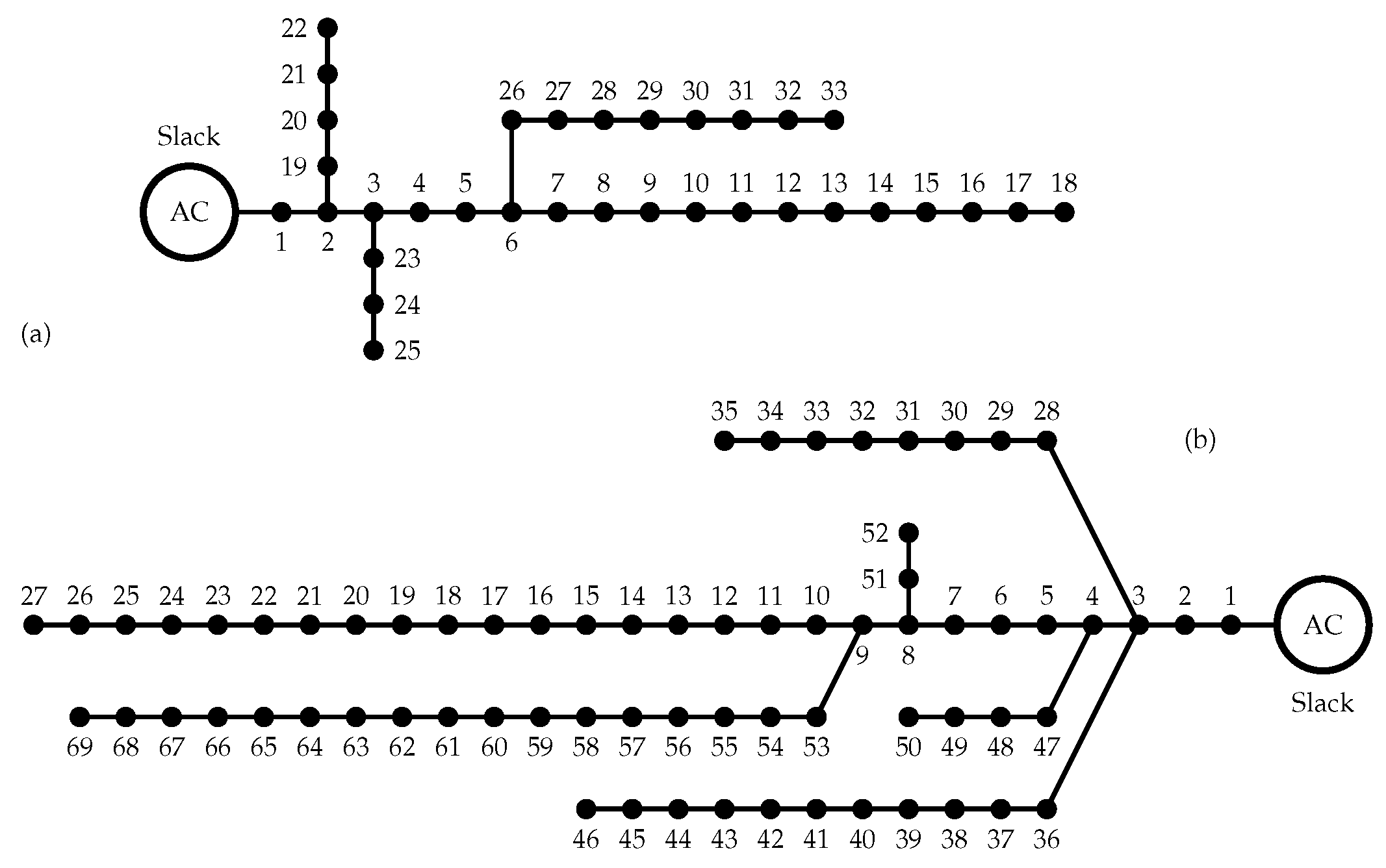
4. Electric Distribution Test Feeders

The evaluation of the proposed MINLP model and the DCVSA to solve the problem of the optimal location and sizing of D-STATCOMs in electric distribution grids is made in two classical and well-known distribution test feeders composed of 33 and 69 buses with radial structure, which will be denominated in this research as the IEEE 33-bus and the IEEE 69-bus, respectively. Both electrical distribution networks are operated with 12.66 kV at the substation node located at bus 1. The schematic connection between nodes in these test feeders are depicted in Figure 1.
The IEEE 33-bus has a total active and reactive power demand of 3715 kW and 2300 kvar with 210.9876 kW of power losses at the peak load condition; while the IEEE 69-bus has a total active and reactive power demand of 3890.7 kW and 2693.6 kvar with 224.9520 kW of power losses in the same operative scenario. All information regarding branches and loads are reported in Table 2 and Table 3 [8].
To evaluate the effect of the daily load variation in both test feeders the active and reactive power curves depicted in Figure 2 are considered.
The information to construct the aforementioned daily active and reactive power curves is presented in Table 4 for the sake of reproducibility of the results that will be presented in the next section.
To evaluate the objective function defined in (1) the parameters reported in Table 5 are considered. Some of these parameters have been taken from [6,33].
It is worth mentioning that in the evaluation of the f 2 component, the variable Q k D - STATCOM is defined in MVAr [33].

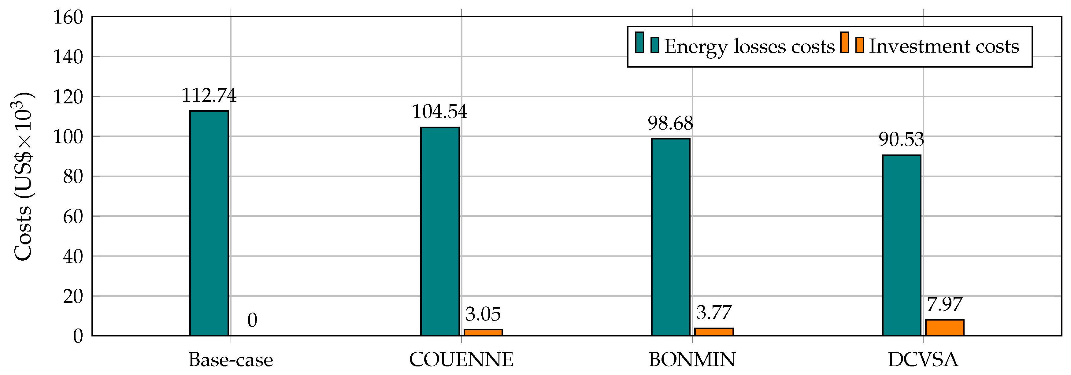
5. Computational Implementation and Results

The solution of the MINLP model (1)–(6) for the optimal siting and sizing of D-STATCOMs in electric distribution networks using the DCVSA was implemented in the MATLAB version 2020b on a PC with an AMD Ryzen 7 3700 2.3-GHz processor and 16.0 GB RAM, running on a 64-bit version of Microsoft Windows 10 Single language. In addition, to compare the efficiency and robustness of the proposed optimization approach the MINLP model was also solved in the GAMS software with BONMIN and COUENNE solvers [9]. The parameterization of the DVSA was taken from [8] and it is presented in Table 6.

5.1. IEEE 33-Bus

In Table 7 are listed the optimal solutions for the problem of the optimal placement and sizing of D-STATCOMs in electric distribution networks using the GAMS optimizers and the proposed optimization DCVSA approach.
Please note that the solutions reported in Table 7 show that: (i) the best solution is reported by the proposed DCVSA with the selection of the nodes 14, 30 and 32 to locate the D-STATCOMs with sizes of 0.1599 MVAr, 0.3591 MVAr, and 0.1072 MVAr, respectively. These reduce the operating cost of the electric distribution grid by about US$14243 per year of operation, i.e., 12.63% with compared to the base case; and (ii) the GAMS solvers are stuck in local optimal solutions. The BONMIN solver reduces the total annual grid cost by about 9.13%, while the COUENNE achieves a reduction of only 4.57%. These problems in the solutions reported by the GAMS solvers are clearly attributable to the nonlinear non-convex behavior of the objective function and the power balance constraints, which makes it impossible to combine classical branch and bound method, which, with interior points, finds the global optimum. This is possible only in mixed-integer convex problems.
To present the effect of the optimal location on the costs of the annual energy losses, we desegregate the investment and the operative costs associated with the installation of the D-STATCOMs reported in Table 7. In the Figure 3 are presented the desegregated costs for the IEEE 33-bus test system.
The behavior of the annual investment and operating costs presented in Figure 3 shows that the proposed DCVSA decides to make an inversion in D-STATCOMs that duplicates the inversion made by the GAMS solvers. However, this behavior of the DCVSA leads to considerable reduction in the cost of annual energy losses and helps to improve the grid behavior significantly as compared with the GAMS solvers. In addition, if we observe the cost of annual energy losses of the BONMIM solver, these are about US $98.67 × 10³, which is itself higher than the summation of the costs reported with the proposed DCVSA which is about US $98.50 × 10³—This result proves that the proposed approach is more suitable for solving complex mixed-integer non-convex optimization problems than the GAMS package as shown in [9].
To demonstrate the efficiency of the proposed DCVSA we report the first six solutions found by this approach in Table 8.
Please note that the results in Table 8 demonstrate that: (i) after 100 consecutive evaluations, the proposed DCVSA is found to have a 36% efficiency at finding the same optimal solution, (ii) all the solutions in Table 8 are indeed better than the results achieved by the GAMS optimizers in reaching the final objective function value, and (iii) it is observed that the node 30 appears in all the solutions with sizes larger than 350 kvar, which implies that this is the most sensitive node for the placement of D-STATCOMs in the IEEE 33-bus test system.
It is also important to mention that about processing times the proposed approach takes about 76.85 s to solve the optimization problem with excellent numerical results in contrast with the 6.6 s taken by the BONMIN solver that is stuck in a local solution which is worse than all the solutions listed in Table 8.

5.2. IEEE 69-Bus

To present the effectiveness and robustness of the proposed DCVSA to solve the problem of the optimal siting and sizing of D-STATCOMs in the IEEE 69-bus test feeder, first six solutions reached by our proposed method are presented in Table 9. Please note that the base case for this test feeder has an annual cost of US $119,715.63.
Regarding the solutions reported in Table 9 it is observed that: (i) in all the solutions the node 61 and 21 are recur, except in solution 2 where node 17 replaces node 21, which implies that these are the most suitable nodes to locate D-STATCOMs. On the basis of maximum reduction in the annual operating costs, node 61 with the D-STATCOM of the largest size appears in all the simulation cases; (ii) the solutions 3 to 6 are comparable because the differences among their annual costs are less than US $0.4100 per year of operation and the fact that in all these node 61 node features as the location for a D-STATCOM with a nominal rate of 0.5741 MVAr; and (iii) the proposed optimization approach for the IEEE 69-bus test system has an efficiency of the 49%, i.e., among 100 consecutive evaluations, 49 find global optimal solutions that cause the reduction of about 13.97% in the annual operative cost as compared to the base case when D-STATCOMs are installed at nodes 61, 61 and 64 with nominal rates of 0.0839 MVAr, 0.4601 MVAr, and 0.1139 MVAr, respectively.
Remark 5.
Comparisons with the GAMS solvers are not presented since the BONMIN and the COUENNE failed to solve the MINLP model for the IEEE 69-bus test feeder. This further demonstrates the efficiency and robustness of the DCVSA for addressing this complex optimization problem from the meta-heuristic optimization point of view.
If we split the optimal solution yield by the proposed DCVSA in Table 9, then, the required inversion in D-STATCOMs is US $8372.08 against the reduction in the costs of the energy losses of US $25,096.92 seen in the base case. This clearly compensates for the required inversions in the D-STATCOMs, because it leads to a reduction of 13.97% in the annual operating costs for the grid operator, i.e., US $16,724.84 per year of operation.
It is also important to mention the processing times the proposed approach takes. It is about 300.68 s to solve the optimization problem with excellent numerical results while the GAMS solvers diverge after 2187.96 s of exploration in the solution space.

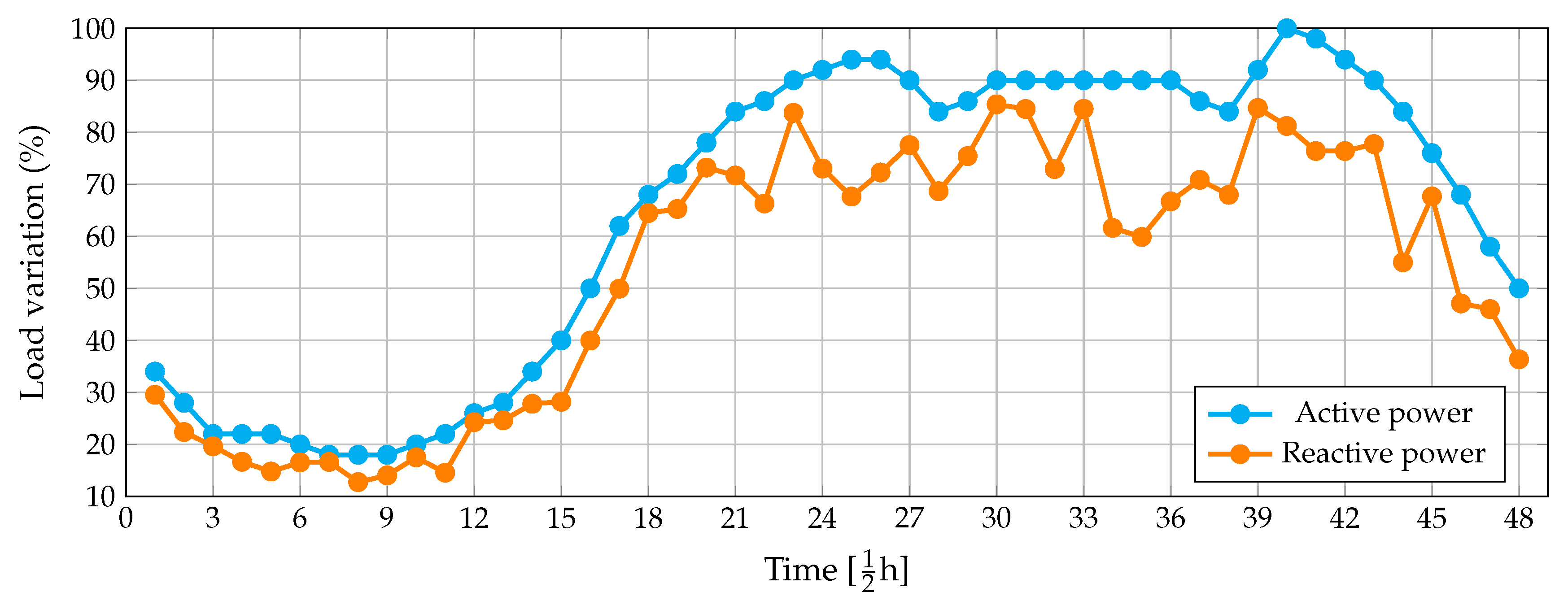
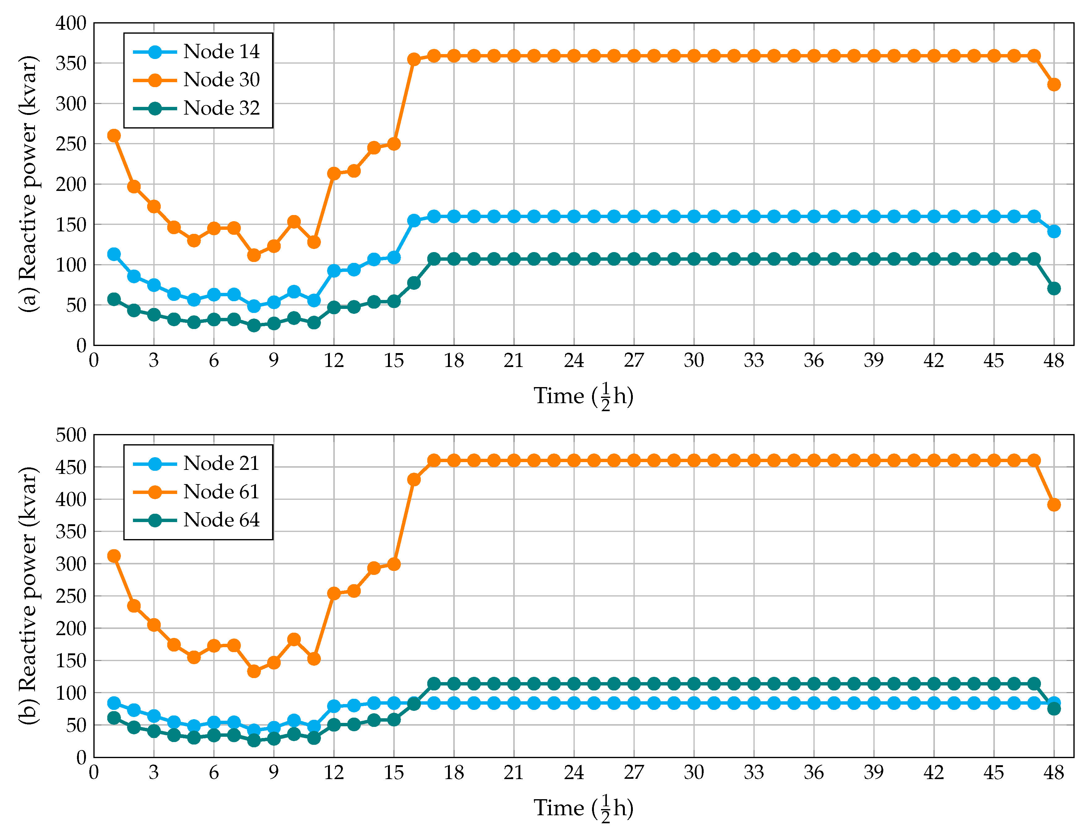
5.3. Daily Operation of the D-STATCOMs

To verify the dynamic behavior of the D-STATCOMs in the reactive power compensation in electric distribution systems considering the daily active and reactive power demand curves presented in Figure 2, we present the D-STATCOMs’ behavior in Figure 4a,b for the IEEE 33- and 69-buses test feeders, respectively.
From results in Figure 4 it may be noted that: (i) for the IEEE 33-bus test feeder all the D-STATCOMs work in their nominal capacities from the periods 16 to 47, while for the other periods, the amount of reactive power varies as a function of the total active and reactive power demand because, for these periods (see period 1 to period 16 in Figure 2), the total active and reactive power consumption is lower than the 50%. This implies that excessive injections of reactive power can worsen the grid performance in terms of energy losses; (ii) with the daily operation of the D-STATCOMs presented in Figure 4 the annual energy costs also reduced from US $90,527.63 to US $89,314.22, i.e., an additional reduction of about USD 1231.41 per year of operation; (iii) in the IEEE 69-bus test feeder the dynamic behavior of the D-STATCOMs shows that during the periods 1 to 17 and in the last, i.e., the 47th period, the amount of the reactive power injection was lower than the nominal rates of the D-STATCOMs. This was caused by the low demand in these periods of time (see Figure 2); and (iv) if the D-STATCOMs are operated throughout the day at their nominal values (see Table 9) the cost of annual energy losses is about US $94,618.71. If, however, these are operated with the dynamic curves presented in Figure 4b, then, the cost of annual energy losses is about US $93,027.84, i.e., an additional reduction of US $1590.87 per year of operation.
It is also important to mention that the dynamic behavior of the reactive power injections in Figure 4 in the IEEE 33- and IEEE 69-bus test feeder confirms the advantages of using D-STATCOMs instead fixed capacitor banks because the former can vary their reactive power injections as function of the demand demeanor, which is not possible when fixed capacitors are installed.

6. Conclusions and Future Works

The problem of the optimal siting and sizing of D-STATCOMs in electric distribution networks to minimize the annual operational costs of the grid caused by the energy losses during a typical day of operation was formulated as an MINLP model in research. The model proposed in this study incorporates of the a new version of the VSA that uses a discrete-continuous codification (DCVSA) and the SAPF method. The DCVSA is used for determining the optimal locations for and sizes of the D-STATCOMs and the SAPF method entrusted determines the voltage variables to calculate the annual energy losses of the grid and their cost. Numerical results in the IEEE 33- and IEEE 69-bus test feeders demonstrated that the proposed hybrid optimization approach showed a better numerical performance than the MINLP solvers BONMIN and COUENNE in the GAMS package. With the IEEE 33-bus test feeder, the DCVSA caused an annual reduction about 12.63%, while the BONMIN and the COUENNE solvers could bring about reductions of about 9.13% and 4.57%, respectively. With the IEEE 69-node test feeder, the reduction with DCVSA was about 13.97% and that with the GAMS solvers was variable.
The evaluation of the dynamic reactive power compensation using the D-STATCOMs sized and located by the proposed DCVSA approach showed that depending on the amount of active and reactive power demands throughout the day, the reactive power injection must be varied to achieve even greater improvement in the annual performance of the grid. Numerical results showed that for the IEEE 33-bus and IEEE 69-bus test feeders, additional annual reductions of about US $1231.41 and US $1590.87 were achieved as compared to fixed reactive power injections.
As future works, the following research topics may explore: (i) the reformulation of the MINLP model into a mixed-integer convex model to find the global optimum with the application of the Branch and Bound and the interior point methods; and (ii) the simultaneous location and sizing of the renewable energy resources and D-STATCOMs to improve the grid performance during the planning horizon, considering annual load increments.

Author Contributions

Conceptualization, O.D.M. and W.G.-G.; Methodology, O.D.M. and W.G.-G.; Investigation, O.D.M., W.G.-G. and J.C.H.; Writing—review and editing, O.D.M., W.G.-G. and J.C.H. All authors have read and agreed to the published version of the manuscript.

Funding

This research was funded by the Centro de Investigación y Desarrollo Científico de la Universidad Distrital Francisco José de Caldas under grant 1643-12-2020 associated with the project: “Desarrollo de una metodología de optimización para la gestión óptima de recursos energéticos distribuidos en redes de distribución de energía eléctrica.”

Acknowledgments

This work was supported in part by the Dirección de Investigaciones de la Universidad Tecnológica de Bolívar under grant PS2020002 associated with the project: “Ubicación óptima de bancos de capacitores de paso fijo en redes eléctricas de distribución para reducción de costos y pérdidas de energía: Aplicación de métodos exactos y metaheurísticos.”

Conflicts of Interest

The authors declare no conflict of interest.

References

  1. Alam, M.S.; Arefifar, S.A. Energy Management in Power Distribution Systems: Review, Classification, Limitations and Challenges. IEEE Access 2019, 7, 92979–93001. [Google Scholar] [CrossRef]
  2. Montoya, O.D.; Gil-González, W. Dynamic active and reactive power compensation in distribution networks with batteries: A day-ahead economic dispatch approach. Comput. Electr. Eng. 2020, 85, 106710. [Google Scholar] [CrossRef]
  3. Montoya, O.; Gil-González, W.; Garces, A. Numerical methods for power flow analysis in DC networks: State of the art, methods and challenges. Int. J. Electr. Power Energy Syst. 2020, 123, 106299. [Google Scholar] [CrossRef]
  4. Sadovskaia, K.; Bogdanov, D.; Honkapuro, S.; Breyer, C. Power transmission and distribution losses—A model based on available empirical data and future trends for all countries globally. Int. J. Electr. Power Energy Syst. 2019, 107, 98–109. [Google Scholar] [CrossRef]
  5. Montoya, O.D.; Serra, F.M.; Angelo, C.H.D. On the Efficiency in Electrical Networks with AC and DC Operation Technologies: A Comparative Study at the Distribution Stage. Electronics 2020, 9, 1352. [Google Scholar] [CrossRef]
  6. Marjani, S.R.; Talavat, V.; Galvani, S. Optimal allocation of D-STATCOM and reconfiguration in radial distribution network using MOPSO algorithm in TOPSIS framework. Int. Trans. Electr. Energy Syst. 2018, 29, e2723. [Google Scholar] [CrossRef]
  7. Tolabi, H.B.; Ali, M.H.; Rizwan, M. Simultaneous Reconfiguration, Optimal Placement of DSTATCOM, and Photovoltaic Array in a Distribution System Based on Fuzzy-ACO Approach. IEEE Trans. Sustain. Energy 2015, 6, 210–218. [Google Scholar] [CrossRef]
  8. Gil-González, W.; Montoya, O.D.; Rajagopalan, A.; Grisales-Noreña, L.F.; Hernández, J.C. Optimal Selection and Location of Fixed-Step Capacitor Banks in Distribution Networks Using a Discrete Version of the Vortex Search Algorithm. Energies 2020, 13, 4914. [Google Scholar] [CrossRef]
  9. Montoya, O.D.; Molina-Cabrera, A.; Chamorro, H.R.; Alvarado-Barrios, L.; Rivas-Trujillo, E. A Hybrid Approach Based on SOCP and the Discrete Version of the SCA for Optimal Placement and Sizing DGs in AC Distribution Networks. Electronics 2020, 10, 26. [Google Scholar] [CrossRef]
  10. Grisales-Noreña, L.; Montoya, O.D.; Ramos-Paja, C.A. An energy management system for optimal operation of BSS in DC distributed generation environments based on a parallel PSO algorithm. J. Energy Storage 2020, 29, 101488. [Google Scholar] [CrossRef]
  11. Sirjani, R.; Jordehi, A.R. Optimal placement and sizing of distribution static compensator (D-STATCOM) in electric distribution networks: A review. Renew. Sustain. Energy Rev. 2017, 77, 688–694. [Google Scholar] [CrossRef]
  12. Saxena, N.K.; Kumar, A. Cost based reactive power participation for voltage control in multi units based isolated hybrid power system. J. Electr. Syst. Inf. Technol. 2016, 3, 442–453. [Google Scholar] [CrossRef] [Green Version]
  13. Gupta, A.R.; Kumar, A. Energy Savings Using D-STATCOM Placement in Radial Distribution System. Procedia Comput. Sci. 2015, 70, 558–564. [Google Scholar] [CrossRef] [Green Version]
  14. Samimi, A.; Golkar, M.A. A Novel Method for Optimal Placement of STATCOM in Distribution Networks Using Sensitivity Analysis by DIgSILENT Software. In Proceedings of the 2011 Asia-Pacific Power and Energy Engineering Conference, Wuhan, China, 25–28 March 2011. [Google Scholar] [CrossRef]
  15. Jazebi, S.; Hosseinian, S.; Vahidi, B. DSTATCOM allocation in distribution networks considering reconfiguration using differential evolution algorithm. Energy Convers. Manag. 2011, 52, 2777–2783. [Google Scholar] [CrossRef]
  16. Devi, S.; Geethanjali, M. Optimal location and sizing determination of Distributed Generation and DSTATCOM using Particle Swarm Optimization algorithm. Int. J. Electr. Power Energy Syst. 2014, 62, 562–570. [Google Scholar] [CrossRef]
  17. Devi, S.; Geethanjali, M. Placement and Sizing of D-STATCOM Using Particle Swarm Optimization. In Lecture Notes in Electrical Engineering; Springer: Chennai, India, 2014; pp. 941–951. [Google Scholar] [CrossRef]
  18. Bagherinasab, A.; Zadehbagheri, M.; Khalid, S.A.; Gandomkar, M.; Azli, N.A. Optimal Placement of D-STATCOM Using Hybrid Genetic and Ant Colony Algorithm to Losses Reduction. Int. J. Appl. Power Eng. 2013, 2. [Google Scholar] [CrossRef]
  19. Singh, B.; Singh, S. GA-based optimization for integration of DGs, STATCOM and PHEVs in distribution systems. Energy Rep. 2019, 5, 84–103. [Google Scholar] [CrossRef]
  20. Karami, H.; Zaker, B.; Vahidi, B.; Gharehpetian, G.B. Optimal Multi-objective Number, Locating, and Sizing of Distributed Generations and Distributed Static Compensators Considering Loadability using the Genetic Algorithm. Electr. Power Compon. Syst. 2016, 44, 2161–2171. [Google Scholar] [CrossRef]
  21. Rukmani, D.K.; Thangaraj, Y.; Subramaniam, U.; Ramachandran, S.; Elavarasan, R.M.; Das, N.; Baringo, L.; Rasheed, M.I.A. A New Approach to Optimal Location and Sizing of DSTATCOM in Radial Distribution Networks Using Bio-Inspired Cuckoo Search Algorithm. Energies 2020, 13, 4615. [Google Scholar] [CrossRef]
  22. Yuvaraj, T.; Ravi, K.; Devabalaji, K.R. Optimal Allocation of DG and DSTATCOM in Radial Distribution System Using Cuckoo Search Optimization Algorithm. Model. Simul. Eng. 2017, 2017, 2857926. [Google Scholar] [CrossRef] [Green Version]
  23. Nguyen, K.P.; Fujita, G.; Dieu, V.N. Cuckoo Search Algorithm for Optimal Placement and Sizing of Static Var Compensator in Large-Scale Power Systems. J. Artif. Intell. Soft Comput. Res. 2016, 6, 59–68. [Google Scholar] [CrossRef] [Green Version]
  24. Yuvaraj, T.; Ravi, K. Multi-objective simultaneous DG and DSTATCOM allocation in radial distribution networks using cuckoo searching algorithm. Alex. Eng. J. 2018, 57, 2729–2742. [Google Scholar] [CrossRef]
  25. Taher, S.A.; Afsari, S.A. Optimal location and sizing of DSTATCOM in distribution systems by immune algorithm. Int. J. Electr. Power Energy Syst. 2014, 60, 34–44. [Google Scholar] [CrossRef]
  26. Yuvaraj, T.; Devabalaji, K.; Ravi, K. Optimal Placement and Sizing of DSTATCOM Using Harmony Search Algorithm. Energy Procedia 2015, 79, 759–765. [Google Scholar] [CrossRef] [Green Version]
  27. Zhang, T.; Xu, X.; Li, Z.; Abu-Siada, A.; Guo, Y. Optimum Location and Parameter Setting of STATCOM Based on Improved Differential Evolution Harmony Search Algorithm. IEEE Access 2020, 8, 87810–87819. [Google Scholar] [CrossRef]
  28. Sedighizadeh, M.; Eisapour-Moarref, A. The Imperialist Competitive Algorithm for Optimal Multi-Objective Location and Sizing of DSTATCOM in Distribution Systems Considering Loads Uncertainty. INAE Lett. 2017, 2, 83–95. [Google Scholar] [CrossRef] [Green Version]
  29. Montoya, O.D.; Gil-González, W. On the numerical analysis based on successive approximations for power flow problems in AC distribution systems. Electr. Power Syst. Res. 2020, 187, 106454. [Google Scholar] [CrossRef]
  30. Doğan, B.; Ölmez, T. Vortex search algorithm for the analog active filter component selection problem. AEU—Int. J. Electron. Commun. 2015, 69, 1243–1253. [Google Scholar] [CrossRef]
  31. Özkış, A.; Babalık, A. A novel metaheuristic for multi-objective optimization problems: The multi-objective vortex search algorithm. Inf. Sci. 2017, 402, 124–148. [Google Scholar] [CrossRef]
  32. Montoya, O.D.; Gil-Gonzalez, W.; Grisales-Norena, L.F. Vortex Search Algorithm for Optimal Power Flow Analysis in DC Resistive Networks with CPLs. IEEE Trans. Circuits Syst. II Express Briefs 2020, 67, 1439–1443. [Google Scholar] [CrossRef]
  33. Sharma, A.K.; Saxena, A.; Tiwari, R. Optimal Placement of SVC Incorporating Installation Cost. Int. J. Hybrid Inf. Technol. 2016, 9, 289–302. [Google Scholar] [CrossRef]
Figure 1. Nodal connections of the test feeder (a) IEEE 33-bus (b) IEEE 69-bus.
Applsci 11 02175 g001
Figure 2. Typical behavior of the active and reactive power consumption in Colombia [2].
Applsci 11 02175 g002
Figure 3. Distribution of the operative and investment costs for the comparative and proposed approach.
Applsci 11 02175 g003
Figure 4. Dynamic reactive power behavior in a typical operation day for the D-STATCOMs in electric distribution networks: (a) IEEE 33-bus, and (b) IEEE 69-bus.
Applsci 11 02175 g004
Table 1. Meta-heuristic approaches applied to the optimal location and sizing of D-STATCOMs in electric distribution networks.
Optimization TechniqueRefs.
Particle swarm optimization[6,16,17]
Genetic algorithms[14,18,19,20]
Cuckoo search algorithm[21,22,23,24]
Immune algorithm[25]
Harmony search algorithm[26,27]
Imperialist competitive algorithm[28]
Table 2. Electrical parameters of the 33-node test feeder.
Node iNode jRij (Ω)Xij (Ω)Pj (kW)Qj (kvar)Node iNode jRij (Ω)Xij (Ω)Pj (kW)Qj (kvar)
120.09220.04771006017180.73200.57409040
230.49300.251190402190.16400.15659040
340.36600.18641208019201.50421.35549040
450.38110.1941603020210.40950.47849040
560.81900.7070602021220.70890.93739040
670.18720.61882001003230.45120.30839050
781.71141.235120010023240.89800.7091420200
891.03000.7400602024250.89600.7011420200
9101.04000.740060206260.20300.10346025
10110.19660.0650453026270.28420.14476025
11120.37440.1238603527281.05900.93376020
12131.46801.1550603528290.80420.700612070
13140.54160.71291208029300.50750.2585200600
14150.59100.5260601030310.97440.963015070
15160.74630.5450602031320.31050.3619210100
16171.28901.7210602032330.34100.53026040
Table 3. Electrical parameters of the 69-node test feeder.
Node iNode jRij (Ω)Xij (Ω)Pj (kW)Qj (kvar)Node iNode jRij (Ω)Xij (Ω)Pj (kW)Qj (kvar)
120.00050.0012003360.00440.01082618.55
230.00050.00120036370.06400.15652618.55
340.00150.00360037380.10530.123000
450.02510.02940038390.03040.03552417
560.36600.18642.62.239400.00180.00212417
670.38100.194140.43040410.72830.85091.21
780.09220.0470755441420.31000.362300
890.04930.0251302242430.04100.047564.3
9100.81900.2707281943440.00920.011600
10110.18720.061914510444450.10890.137339.2226.3
11120.71140.235114510445460.00090.001239.2226.3
12131.03000.3400854470.00340.008400
13141.04400.345085.547480.08510.20837956.4
14151.05800.34960048490.28980.7091384.7274.5
15160.19660.065045.53049500.08220.2011384.7274.5
16170.37440.123860358510.09280.047340.528.3
17180.00470.0016603551520.33190.11143.62.7
18190.32760.1083009530.17400.08864.353.5
19200.21060.069010.653540.20300.103426.419
20210.34160.11291148154550.28420.14472417.2
21220.01400.004653.555560.28130.143300
22230.15910.05260056571.59000.533700
23240.34600.1145282057580.78370.263000
24250.74880.24750058590.30420.100610072
25260.30890.1021141059600.38610.117200
26270.17320.0572141060610.50750.25851244888
3280.00440.01082618.661620.09740.04963223
28290.06400.15652618.662630.14500.073800
29300.39780.13150063640.71050.3619227162
30310.07020.02320064651.04100.53025942
31320.35100.11600011660.20120.06111813
32330.83900.2816141066670.00470.00141813
33341.70800.564619.51412680.73940.24442820
34351.47400.48736468690.00470.00162820
Table 4. Behavior of the daily active and reactive power demands.
PeriodAct. (pu)React. (pu)PeriodAct. (pu)React. (pu)
10.17000.1477250.47000.3382
20.14000.1119260.47000.3614
30.11000.0982270.45000.3877
40.11000.0833280.42000.3434
50.11000.0739290.43000.3771
60.10000.0827300.45000.4269
70.09000.0831310.45000.4224
80.09000.0637320.45000.3647
90.09000.0702330.45000.4226
100.10000.0875340.45000.3081
110.11000.0728350.45000.2994
120.13000.1214360.45000.3336
130.14000.1231370.43000.3543
140.17000.1390380.42000.3399
150.20000.1410390.46000.4234
160.25000.1998400.50000.4061
170.31000.2497410.49000.3820
180.34000.3224420.47000.3820
190.36000.3263430.45000.3887
200.39000.3661440.42000.2751
210.42000.3585450.38000.3383
220.43000.3316460.34000.2355
230.45000.4187470.29000.2301
240.46000.3652480.25000.1818
Table 5. Parametrization of the objective function.
Par.ValueUnitPar.ValueUnit
CkWh0.1390US$kWhT365Days
Δh0.50hα0.30US$/MVAr3
β−305.10US$/MVAr2γ127,380US$/MVAr
k16/21901/Daysk210Years
Table 6. Parametrization of the DCVSA.
Discrete-continuous vortex search algorithm
Population size: 10Iterations’ number: 1000
Population building: Gaussian Distribution
SAPF method
Iterations’ number: 1000Convergence error: 1 × 10⁻¹⁰
Experimental tests in each test feeder
Consecutive evaluations100
Table 7. Optimal location and sizes of the D-STATCOMs in the IEEE 33-bus.
ApproachLocation and Size Node (MVAr)Acost
(US $/Year)
Caso base112,740.90
COUENNE{16(0.0109), 17(0.0224), 18(0.2065)}107,589.50
BONMIN{17(0.0339), 18(0.0227), 30(0.2395)}102,447.29
DCVSA {14(0.1599), 30(0.3591), 32(0.1072)}98,497.90
Table 8. Lists of solutions found by the proposed DCVSA in the IEEE 33-bus.
Sol.Location and Size Node (MVAr)Acost
(US $/Year)
Rep.
1{14(0.1599), 30(0.3591), 32(0.1072)}98,497.9036
2 {11(0.0659), 14(0.1148), 30(0.4578)}98,564.2922
3{10(0.0642), 14(0.1175), 30(0.4574)}98,565.0310
4{11(0.0787), 15(0.1019), 30(0.4578)}98,567.918
5{12(0.1110), 14(0.0666), 30(0.4591)}98,569.082
6{12(0.0804), 15(0.0972), 30(0.4591)}98,570.124
Table 9. Lists of solutions found by the proposed DCVSA in the IEEE 69-bus.
Sol.Location and Size Node (MVAr)Acost
(US $/Year)
Rep.
1{21(0.0839), 61(0.4601), 64(0.1139)}102,990.8049
2{17(0.0862), 61(0.4597), 64(0.1139)}103,022.771
3{21(0.0695), 26(0.0143), 61(0.5741)}103,101.253
4{21(0.0704), 27(0.0134), 61(0.5741)}103,101.311
5{21(0.0687), 25(0.0152), 61(0.5741)}103,101.521
6{22(0.0695), 26(0.0143), 61(0.5741)}103,101.664
Publisher’s Note: MDPI stays neutral with regard to jurisdictional claims in published maps and institutional affiliations.

