Prediction of Mean Responses of RC Bridges Considering the Incident Angle of Ground Motions and Displacement Directions


1
Department of Civil and Environmental Engineering, Amirkabir University of Technology (Tehran Polytechnic), 424 Hafez Ave, Tehran 15875-4413, Iran
2
Department of Civil Engineering & Applied Mech., McGill University, Montreal, QC H3A 0C3, Canada
*
Author to whom correspondence should be addressed.
Appl. Sci. 2021, 11(6), 2462; https://0-doi-org.brum.beds.ac.uk/10.3390/app11062462
Submission received: 24 February 2021
/
Revised: 5 March 2021
/
Accepted: 5 March 2021
/
Published: 10 March 2021
(This article belongs to the Special Issue Bridge Dynamics: Volume II)
Abstract
:Featured Application
Results from this study indicate that in a 3D time history analysis, without considering the directionality of the records, the actual maximum displacements occur in a random direction and they are around 20% larger than those predicted in the principal axes of the structure, based on the current design practice. When the directivity effects are also considered in the analysis, the difference can increase up to 70% compared to the displacements predicted in the principal X and Y directions. This difference may be more significant for different types of structures, particularly irregular structures. These issues need to be considered in the seismic design and analysis of bridges.
Abstract
Inelastic dynamic analyses were carried out using 3D and 2D models to predict the mean seismic response of four-span reinforced concrete (RC) bridges considering directionality effects. Two averaging methods, including an advanced method considering displacement direction, were used for the prediction of the mean responses to account for different incident angles of ground motion records. A method was developed to predict the variability of the mean displacement predictions due to variability in the incident angles of the records for different averaging methods. When the concepts of averaging in different directions were used, significantly different predictions were obtained for the directionality effects. The accuracy of the results obtained using 2D and 3D analyses with and without the application of the combination rules for the prediction of the mean seismic demands considering the incident angle of the records was investigated. The predictions from different methods to account for the records incident angles were evaluated probabilistically. Recommendations were made for the use of the combination rules to account for the directivity effects of the records and to predict the actual maximum displacement, referred to as the maximum radial displacement.
1. Introduction
Nonlinear dynamic analysis is widely used for predicting the seismic response of structures and it is typically performed using either 2D or 3D structural models. Different methods for applying ground motion records are observed for performing 2D and 3D analysis. This research is intended to investigate and compare the results obtained using different methods currently used in research and practice. Some issues are not very well addressed in seismic codes, including the effects of directivity of records in 2D and 3D analysis, the use of different combination rules for prediction of inelastic displacements and the methods for predicting the mean response of structures subjected to a number of records at different incident angles.
In design, it is often assumed that the seismic response of straight bridges is independent in the two orthogonal directions and therefore the seismic responses in the two principal directions can be predicted using 2D analysis with the application of horizontal components of the ground motion records applied separately in the transverse and in the longitudinal directions (e.g., [1]). In addition, different methods are available to predict the mean values of seismic demands when structural models are subjected to seven or more records. The use of different averaging methods for the prediction of the mean response of bridges (i.e., averaging the maximum absolute value displacements and averaging the displacements in different directions) is investigated in this study and the predictions from different methods are compared.
Seismic analysis results, including the maximum responses, are typically obtained only for the two perpendicular principal directions of a structure. As a result, the actual maximum vectorial displacement, referred to as the “radial displacement” in this paper, for each record is not predicted during the analysis. The radial displacement, Δi, at each time interval i, is calculated according to , where Δix and Δiy are the displacements in the x and y directions, respectively. Therefore the maximum overall displacements are often estimated using the 30% rule (i.e., the combination of 100% response in one direction with 30% of response in the perpendicular direction) or the square root of the sum of the squares (SRSS) combination of the results from the two principal axes of the structure (e.g., [2,3]). The use of such combination rules is an attempt to account for the fact that the maximum displacements in the two principal directions do not occur at the same time. In this study the radial displacements of the bridge columns are determined by post processing the analysis results at each time step (small time steps were considered for this purpose). As a result, the maximum radial displacements (i.e., actual seismic demands) are determined for each record and the results are compared to the predictions obtained using the simplified methods such as the 30% combination rule. It is noted that only the horizontal displacements of columns are considered in this paper, since the vertical displacements are negligible.
It is customary to apply the ground motion records in the principal axes of the structure with no attempt to investigate the variation of the seismic responses as the direction of the applied records changes. This issue is particularly important for bridges, because the seismic responses of the bridges in the transverse and longitudinal directions are typically significantly different.
One of the important parameters that should be considered in seismic analysis and design of bridges is the direction of the input ground motions. Penzien and Watabe [4] demonstrated that since the location of the epicenter of an earthquake is unknown, the direction of the applied earthquake excitations cannot be predicted. In recent years, the directional and orthogonal effects in seismic response of structures have been studied by some researchers to predict the critical angle of excitation for seismic analysis. To account for directivity effects some studies recommend applying the ground motion records in two perpendicular directions and combining the results using a combination rule (e.g., 100–30 percentage rule, 100–40 percentage rule and Square Root of the Sum of the Squares (SRSS) method) to somehow account for the uncertainty due to directionality effects. Such combination rules are often based on experience and have no theoretical basis. Therefore, the use of such rules may result in an underestimation of the seismic response for different structures.
Lopez and Torres [5] in 1997 proposed a simple method to determine the critical angle of seismic incidence and the corresponding peak response of structures subjected to two horizontal components applied along any arbitrary directions for elastic response spectrum analyses. Menun and Der Kiureghian [6] in 1998 developed a new general combination rule for the multi-component excitation called complete quadratic combination with three components (CQC3) and showed that the use of this rule results in improved predictions. Lopez et al. [7] in 2000 developed a formula, using the CQC3 method, to predict the maximum response of structures in a multi-component response spectrum analysis. Anastassiadis et al. [8] in 2002 proposed a design procedure for predicting the critical direction and maximum responses under bi-directional seismic excitations. Athanatopoulou [9] in 2005 showed that imposing ground motions with various incident angles may increase the maximum response of structure up to 80%. Rigato and Medina [10] in 2007 concluded that applying ground motion records with different angles can result in up to 60% difference in prediction of the engineering demand parameters (EDPs) in asymmetrical buildings.
Maleki and Bisadi [11] in 2006 investigated the orthogonal effects in linear seismic analyses of skewed bridges using three ground motion records and compared the predictions of different combination rules. They concluded that the use of 100–40% rule was satisfactory only for the response spectrum analysis, while for the linear time history analyses none of the combination rules were able to predict the maximum response obtained using three records.
All studies mentioned so far investigated the directivity effects using elastic analyses. Bisadi and Head [12] in 2010 evaluated the importance of orthogonal effects in nonlinear time history analyses of single-span straight bridges using three ground motion records and demonstrated that nonlinear analyses are more sensitive to the directivity effects than are linear analyses. Similar results for the use of nonlinear analyses were observed in a study by Moschonas and Kappos [13] in 2013.
In a study by Bisadi and Head [14] in 2011 the use of different combination rules such as the 30% rule, the 40% rule and the SRSS rule for the prediction of maximum response was investigated. The result of that study indicated that the use of these combination rules with nonlinear analyses performed using pairs of records tends to overestimate the predicted maximum response. The use of combination rules was recommended for 2D analyses performed using the horizontal component of ground motion (the component with the larger PGA) in each principal direction of the bridges [14].
Khaled et al. [15,16] in 2011 investigated the use of combination rules for the seismic evaluation of two span bridges, located in different cities with different seismicity levels, and concluded that different combination rules may be appropriate for different locations (i.e., the use of 100–20% and 100–40% for bridges in different regions were recommended, rather than using 100–30% rule for all structures).
Mackie et al. [17] in 2011 demonstrated that the significance of orthogonal effects in bridge structures depends on the structural properties as well as the number of ground motion records used in the analysis.
The directionality effects on the probability of exceeding different damage states and fragility curves have also been studied by some researchers. Banerjee and Shinozuka [18] in 2011 concluded that the critical angle of seismic excitation does not coincide the principal orthogonal axes of bridges and ground motion directionality is an important parameter in predicting the probability of damage. Torbol and Shinozuka [19,20] in 2012 and 2014 demonstrated that ground motion directionality effects can influence the median fragility values by 66%. A study by Taskari and Sextos [21] in 2015 demonstrated that the orthogonal effects have a more significant influence on the fragility curves of individual components of the bridge compared to the fragility of the bridge system. A study by Emami and Halabian [22] in 2015 on regular buildings demonstrated that the maximum engineering demand parameter (EDP) values were increased up to 39% when both the effects of ground motion directionality and spatial distribution of EDPs were considered simultaneously.
In recent years more researchers studied the influence of incident angle of ground motion records on fragility analysis of different types of bridges using different modelling assumptions (e.g., [21,23,24,25,26,27,28,29]). The results from these studies indicate that the incident angle of the ground motion records may have a significant influence on the seismic demands in critical components of the bridge, especially in irregular, skewed or horizontally curved bridges and therefore, the seismic fragility of a bridge may be underestimated when the directionality effects are ignored.
While fragility analysis of bridges provides valuable information regarding the probability of damage expected due to directionality effects for existing bridges, more research should be focused on the methods currently used for analysis and design of bridges by codes to properly address the directionality effects in predicting mean seismic demands for seismic design of different types of bridges. One of the key points that is missing in the literature is the fact that the maximum displacement of columns does not necessarily occur in the direction of the principal axes of the bridge, while in most analyses performed in practice and research only displacements along the principal axes of the structures are reported and used for evaluations. This is because current available programs for structural analysis typically report the results only for such principal axes (i.e., X and Y directions). In this research in addition to the displacements in the principal axes of the bridges, the actual maximum displacement of the columns during the time history analysis is predicted by determining the vectorial combination of the displacements in X and Y direction for each time step in the analysis (referred to as the radial displacement) to evaluate different methods. In addition, an advanced averaging technique based on the recommendations by Priestley et al. [1] is used to predict the responses of columns in different directions from 0 to 360°. It is noted that the resulting radial displacement differs from the incident angle for the application of earthquake records (i.e., incident angles from 0 to 180°). In fact, both directivity effects due to application of records in different directions and effects of maximum displacement of columns occurring in different directions for different records are considered in this research to predict the mean seismic response. The combination of these effects have not been considered in the past.
It is noted that the seismic input directivity has been considered in seismic risk assessment procedures for existing buildings (e.g., [30]) and also some new seismic provisions attempt to consider the directivity of records by using the maximum direction spectra in design and requiring the application of the ground motion records in random directions (e.g., [31,32]). However, the directivity effects in the seismic analysis and design of bridges are not considered by the current bridge design codes and more research should be focused on this subject.
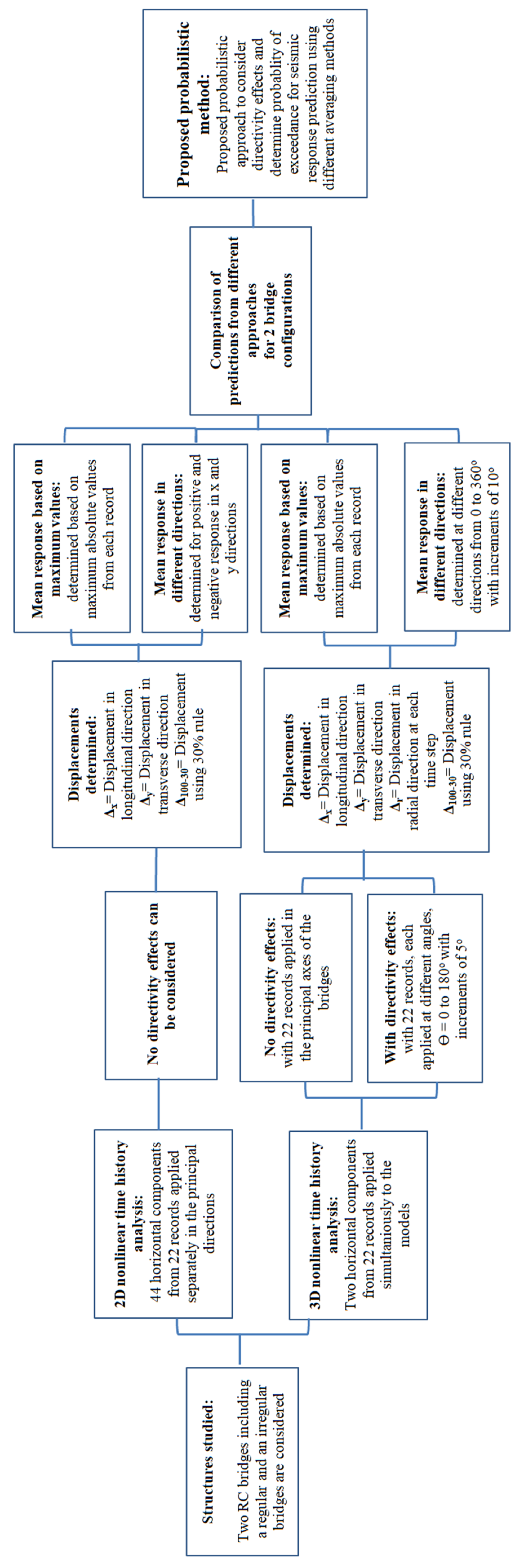
This paper focuses on a detailed examination of directivity of displacements and the directivity of input ground motions as well as different averaging techniques for predicting the mean displacements for a regular and an irregular bridge. Furthermore, the use of different methods for structural analysis including 2D and 3D modeling for considering the directivity effects is studied. Finally, a method is proposed to consider the variability of the mean response due to different excitation angles and to predict the probability of non-exceedance for the results obtained using different averaging methods. A graphical outline of the procedures and steps for this study is presented in Figure 1.
2. Design and Modelling of Bridges
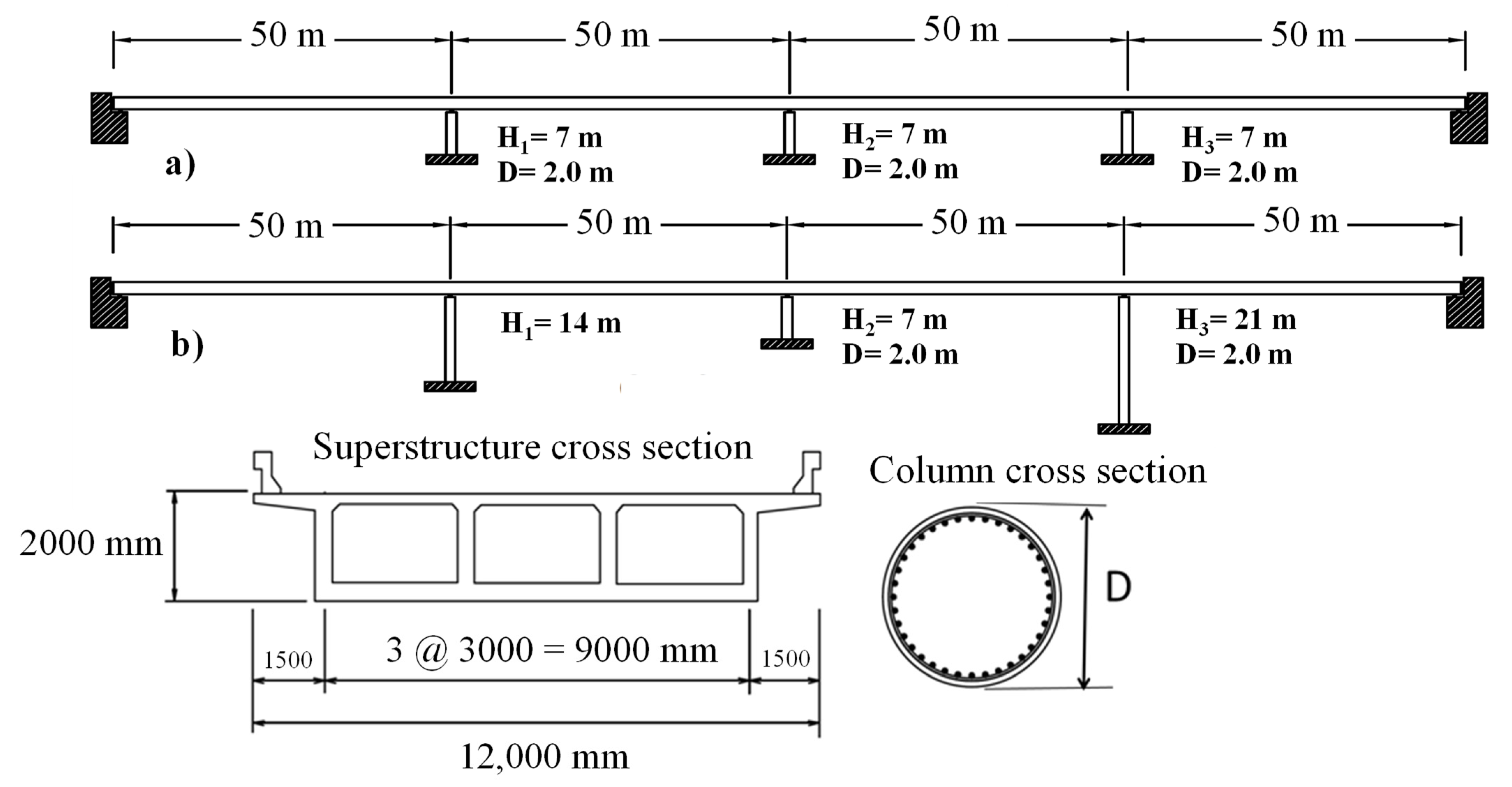
To investigate the influence of using different methods of analysis and different procedures to determine the mean seismic demands using a number of ground motion records, two bridges with different column arrangements were considered. The bridges had four spans with equal lengths of 50 m, as shown in Figure 2, and the superstructure was continuous over the columns. The bridge columns were hinged at the top and fixed at the base. The superstructure consisted of a box girder with a uniform dead load of 200 kN/m. At the abutments the superstructure had no restraint in the longitudinal direction, but was restrained against transverse movements by means of shear keys at the abutments. It is noted that the roller abutment condition in the longitudinal direction can be considered due to the presence of gaps between the superstructure and the abutment back wall (e.g., Roller abutment model discussed by Aviram et al. [33]). The effects of abutment modelling on the seismic response of bridges have been studied by Tehrani and Mitchell [34] based on the abutment models defined by Aviram et al. [33]. However, in the present research, the effects of abutments are neglected in structural modeling because this paper is intended to focus on different subjects including directivity of records, different averaging methods and the use of 2D and 3D analysis. It is noted that similar abutment conditions have been used in many studies (e.g., [1,35,36,37,38,39,40]).
All column diameters were 2.0 m. For the case of the regular bridges, all column heights were 7 m, while for the irregular bridge the column heights were 14, 7 and 21 m. The bridges were designed based on the 2006 Canadian Highway Bridge Design Code (CHBDC) provisions [41] except that the design spectrum given in the 2010 National Building Code of Canada (NBCC) [42] was adopted. The design spectra in the 2010 NBCC corresponds to 2% probability of exceedance in 50 years. The bridges were designed for Vancouver and site class C (i.e., Vs = 555 m/sec) with an importance factor, I of 1.0. The central columns of the regular and irregular bridges contained the longitudinal reinforcement ratios of 1.23% and 1.88%, respectively. All other bridge columns contained the minimum longitudinal reinforcement ratio of 0.8% based on the CHBDC. A confinement reinforcement ratio of 1.2% governed the design of the transverse reinforcement in the columns. The concrete compressive strength and the yield stress of the reinforcing bars were taken as 40 and 400 MPa, respectively. The displacement limit for the critical central columns of the bridges was determined as 370 mm based on the equations developed by Berry and Eberhard [43] for the bar buckling damage state.
In predicting the nonlinear response, the modified Takeda hysteresis model [44] was used in this study to model the behavior of the ductile RC columns using Ruaumoko software [45] using lumped plasticity method, as shown schematically in Figure 3a. This model has two main parameters, alpha and beta, which control the unloading and the reloading stiffness, respectively (see Figure 3b). The values of alpha = 0.5 and beta = 0 were adopted based on the recommendations by Priestley et al. [1]. The structural modelling considered in this study is similar to that used by Priestley et al. [1]. The superstructure was modelled using elastic beam elements and the superstructure mass was lumped at the nodal points as shown in Figure 3a. In addition, the mass of the columns was considered in the corresponding nodal points. Rigid elements were defined to model the superstructure depth. The heights of these elements were considered as half of the superstructure depth (see Figure 3a). For the 3D analyses, the coupling interaction effect of both directions has been considered through the yield interaction of moments with interaction factors of 2 for the circular columns in the Ruaumoko program [45]. The effects of the variation of the axial forces on the seismic response were found to be small for the single-column bridges considered [39,46] and hence were neglected. However, it is noted that although the use of fiber models could more precisely include the interaction effects, such models have difficulty in including realistic shear deformations of columns. Therefore, the use of the modelling adopted in this paper, including the interaction effects, is deemed to provide sufficient accuracy for the sake of this research. The plastic hinge lengths and the strain penetration depths were computed using the equations given by Priestley et al. [1]. To consider the deformations due to bond slippage, the strain penetration depth, Lsp, was considered in modelling, as recommended by Priestley et al. [1,47].
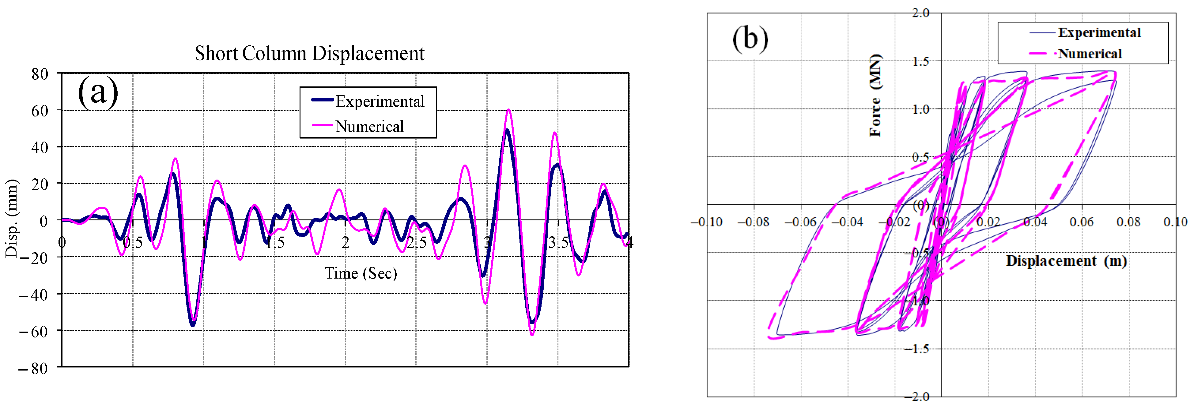
Although this modelling procedure (i.e., using lumped plasticity model) has been widely used in research and practice for design and evaluation of bridges and is recommended in many seismic codes and guidelines such as Caltrans [2] and AASHTO Guide Specifications [3], to further validate the modeling assumptions the numerical results were compared to some experimental data. The data from the RC column tested by Priestley and Benzoni [48] (data were available in the PEER structural database [49]; details are available in [50]) as well as the bridge model labelled as B213C in the experimental study by Pinto et al. [51] were considered to validate the predictions from the numerical models. This large-scale (1:2.5) bridge model was tested in pseudo-dynamic fashion. The experimental data from this test was provided by the European Laboratory for Structural Assessment (ELSA).
A comparison of the results from numerical modelling with experimental results (examples are provided in Figure 4) indicates that the recommendations made by Priestley et al. [1] for modelling bridge structures provided sufficient accuracy in predicting the maximum displacement demands [50]. Therefore, these modelling assumptions were adopted for the seismic analysis and evaluation of the bridges in this research. More details concerning the modelling of the bridges and the verification of computer models are available in [34,40,50,52].
The modal properties of the bridges including the fundamental transverse mode, TT, second transverse mode, TT2, fundamental longitudinal period, TL, geometric mean period, TG, (defined as TG = (TL × TT)0.5) and the effective modal mass ratios are presented in Table 1. It is noted that in the longitudinal direction due to the rigidity of superstructure (i.e., large axial stiffness of the bridge deck) the bridges act similar to a single degree of freedom system and as a result the effective modal mass ratio in the longitudinal direction was almost 100%. The periods are computed using the effective stiffness of the columns (i.e., Ke = My/θy where My and θy are the moment and rotation at yield, respectively).
It is noted that, in this research, regular and irregular four-span bridges were considered only as example cases to investigate the problems discussed in this research, because these types of bridges were the subject of previous studies by the authors (e.g., [34,40,52,53]). Also it should be noted that this study is limited to 2 bridges to demonstrate different methods and present the proposed methodology for considering the variability due to directivity effects for different averaging methods. More research is needed on this subject for a larger number and different types of bridges.
3. Record Selections
Some researchers (e.g., [54]) have expressed their concern about the use of the maximum rotated component spectrum, introduced in the ASCE/SEI Standard 7-10 [55] which may be conservative and may not be consistent with the return period of the design earthquakes in the codes. In this study the method recommended by ASCE/SEI Standard 7-05 [56] was chosen for the selection and scaling of the ground motion records.
For each bridge, 22 pairs of ground motion records (e.g., 44 horizontal components) from the PEER NGA database (http://peer.berkeley.edu/peer_ground_motion_database, accessed in March 2014) were selected. All records were selected from crustal earthquakes, since the effects of earthquake types is not the focus of this paper (e.g., effects of different earthquake types is investigated by Tehrani et al. [57] and Tehrani and Mitchell [40,53]).
It is noted that the latest edition of ASCE-07 provisions [31] require the use of at least 11 records for performing time history analysis. The number of required records was previously 7 records in some older codes (e.g., 2005 edition of ASCE-07 [56]). In this research a larger number of records, including 22 pairs of ground motion records, were used that is much larger than that required by seismic codes. It is noted that a larger number of records were used in this study to make sure that the directivity effects can be appropriately accounted for in the analyses. A sensitivity study by the authors regarding the number of records, which will be presented later in the paper, indicates that the use of 22 records is sufficient for the purpose of this study.
The records in this paper are scaled based on the provisions of ASCE-7 [56] (i.e., amplitude scaling). For this purpose, all of the records in the pool of records were first scaled to match the target spectrum at the geometric mean fundamental period of the bridge, TG. The 22 records with the best matches to the target design spectrum within the period range of interest, that also satisfied the code provisions, were then selected from the pool of records. For measuring the match with the target spectrum within a range of periods the sum of the squared errors between the logarithms of the ground motion’s spectrum and the target spectrum was used as recommended by Baker [58]. A computer program was developed and used to measure the match between the scaled records spectra and the target spectrum within a range of periods and select the records with the closest match that satisfies the code provisions. Although the measurement of matching is not required by seismic codes, this extra step was taken for the purpose of this study to make sure that appropriate records are selected and used to investigate the differences between 2D and 3D analysis.
For each bridge the records were selected so that the average SRSS spectrum of the records matches 1.3 times the design spectrum based on the ASCE-7 provisions [56]. It is noted that the application of the 1.3 factor to the design spectrum is based on the provisions of ASCE 7-05 for performing 3D nonlinear time history analysis. This factor is intended to account for the simultaneous application of horizontal components of records in a 3D analysis. It is also should be noted that the provisions of ASCE 7-05 rather than ASCE 7-10 or ASCE 7-16 were adopted for scaling; because they are compatible with the design spectra in the Canadian codes that do not adopt design spectra based on the maximum direction earthquake. A period range of 0.2T to 3T was used for spectrum matching, where T is the fundamental period of the structure. The smaller fundamental period in the transverse and longitudinal directions was used to determine the lower bound of 0.2T and the larger period was used to determine the upper bound of 3T. It is noted that in the ASCE/SEI Standard 7-10 [55] an upper bound of 2T is recommended for record selection. However, some studies suggest that the period range up to 3T can influence the nonlinear seismic response of ductile structures [59].
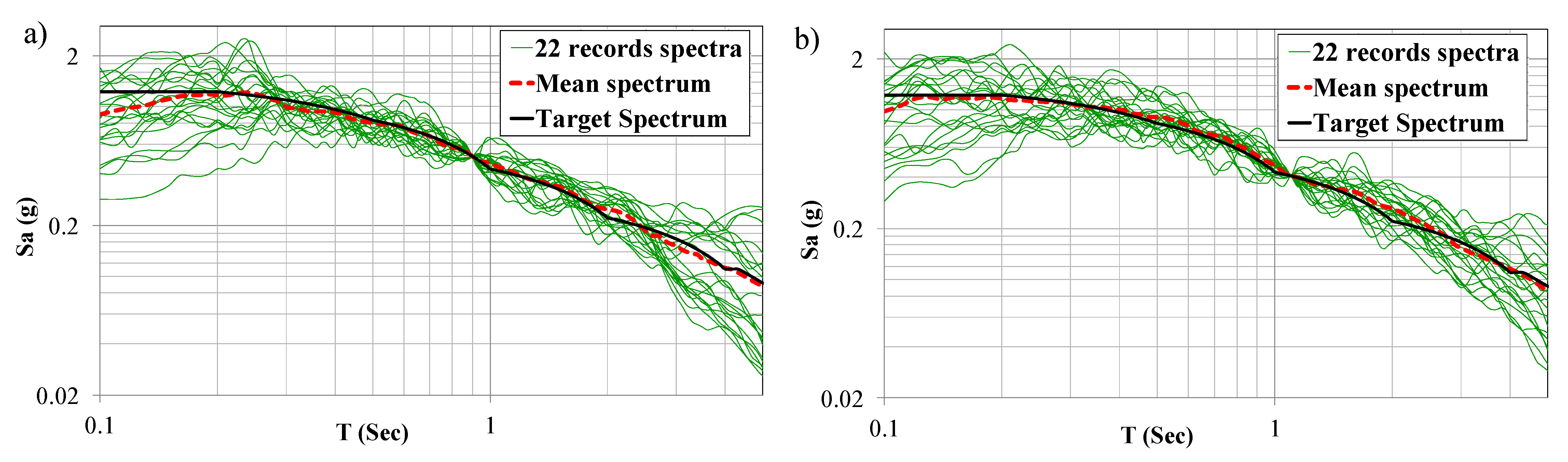
The selected records had a magnitude, M, range of 6.5 to 7.6, a PGA range of 0.11 to 0.54 g, a PGV range of 11 to 54 m/sec, a range of 200 to 725 m/sec and a distance range of 11 to 37 km for the regular bridge. Records corresponding to a distance varying from 13 to 54 km were selected for the irregular bridge during the spectrum matching process. The SRSS response spectra of the selected records, the mean SRSS spectrum of the records and the target spectrum are demonstrated in Figure 5 for the regular and irregular bridges studied. The target spectrum in Figure 5 is determined as 1.3 times the uniform hazard spectrum from the 2010 NBCC [42] for Vancouver having a probability of exceedance of 2% in 50 years.
4. Determining the Mean Responses
In conventional practice the maximum absolute value of deformation is first obtained for each ground motion record and then the mean value from a number of ground motion records are typically used to determine the seismic demands. Priestley et al. [1] recommended that the direction of the displacements should also be considered for calculating the mean response, because displacement is a vector quantity and hence the averaging procedure should consider the direction at which the maximum displacements occur. This more detailed approach enables the determination of realistic values of strains in the concrete and steel corresponding to the resultant vectorial displacement. It is noted that for each time step in the analysis for a record pair, there is an associated predicted displacement that occurs at a particular angle (referred to as the radial direction). From the results of the full time-history of displacements, the maximum displacement in each radial direction (i.e., directions around the full 360°) can be determined for a given ground motion. In this study radial directions at 10° intervals were considered. The average displacement for each radial direction can then be determined for a number of input ground motions. From the mean values in different directions the maximum displacement can be determined [1].
In this study, both of the averaging methods (“average of maximum absolute values” and “average values in different directions”) discussed above are used to determine the mean displacements of the bridge columns.
5. 3D Nonlinear Time History Analysis of Bridges
Structural analysis is typically carried out in the two perpendicular principal directions of the structure (i.e., X and Y directions) and therefore the peak displacements only in the X and Y directions are obtained. Since the peak displacements in the X and Y directions occur at different times, it is not possible to estimate the maximum radial (vectorial) displacement of the columns. In this study the radial displacements were determined at each time interval i, using the component of displacements in X and Y directions (i.e., Δi,r = (Δ2i,x + Δ2i,y)½, where Δi,r is the radial displacement and Δi,x and Δi,y are the displacements in X and Y directions, respectively). Figure 6 shows the time history analysis results for the central column of the regular bridge, shown in Figure 2a, subjected to one of the selected pairs of records for the longitudinal and transverse directions. The computed radial displacements at each time step are also shown in Figure 6. It is noted that, in Figure 6, while the longitudinal and transverse displacements have a sign, the radial displacement is always positive, as calculated using the square root of the sum of the squares of displacements in the principal directions. This is because the radial displacement in Figure 6 only represents the absolute value of the displacements that can occur in a random direction around the full 360°. Further details regarding the direction of the radial displacements are provided in Section 7.
The maximum displacements obtained for the central columns of the bridges from 22 records are presented in Figure 7 and the average values are indicated by black circles. The results are shown using two different averaging methods: using maximum absolute values (see Figure 7a,b); and considering positive and negative displacements in the longitudinal and transverse directions (see Figure 7c,d). The results presented in Figure 7 indicate that when the sign of the displacements is considered the mean predictions are around 10 to 15% smaller compared to the maximum absolute predictions. Also it is clear from Figure 7a,b that the maximum radial displacements are around 13 to 20% larger than the maximum displacements predicted in the principal directions. The predicted average displacements of the bridge columns are summarized in Table 2 for the regular and irregular bridges. The average displacements and corresponding displacement ductility demands are also given in Table 2 for the longitudinal, transverse and radial directions. To determine the ductility demands the predicted maximum displacements, Δmax, were divided by the yield displacement of the columns, Δy (i.e., μ = Δmax/Δy). The yield displacement of the columns was predicted using the equations provided by Priestley et. al. [1] that are also used by the AASHTO guide specifications [3] and Caltrans [2]. The ductility demands are also provided in Table 2, because they are better indicators of damage in columns. A larger ductility demand indicates that a larger plastic deformation, and therefore greater damage is expected in a column. It is noted that, as seen in Table 2, in the longitudinal direction the displacements obtained were similar for all bridge columns due to the large axial stiffness of the superstructure (less than 1% difference observed).
The average responses were predicted using different averaging methods. As presented in Table 2, the predictions obtained using the absolute maximum displacements were significantly larger than those obtained by accounting for the direction of the displacement vectors for the radial displacements. To calculate the mean of absolute maximum values, the maximum response of bridges, regardless of the direction in which they occur, is determined for each record and the mean value from 22 records used in the analysis is reported (i.e., the method that is typically currently used in practice). However, for the case of the average values in different directions, the directions of the displacements are considered (i.e., displacements are treated as vectors) and the displacements of columns are determined in different directions from 0 to 360°. For each record the average of maximum displacements in each direction was determined. For example, in this study the radial directions at 10° intervals were considered and therefore for each record 36 values of maximum displacements in different directions were determined around the full 360°. Finally, the average of 22 values obtained from the 22 records used for the analysis was determined for the 36 directions under consideration. This means that 22 × 36 = 792 values of displacements were involved in this method. The maximum displacement predicted in each direction is then reported (i.e., the maximum of the 36 values determined around the full 360°). To determine the displacement in each direction a computer code was developed for posts processing the analysis results, since current available software typically don’t report such data. It is noted this method accounts for the fact that displacements are vectors and their mean values should consider their direction. Further details regarding the logic of this method are given by Priestley et al. [1]. It is noted that this method has not been typically used in practice and in this paper the applicability of this method is investigated.
For example, the average radial displacement demand for the central column (C2) of the regular bridge was determined as 123 mm using the absolute displacements from different records and 84 mm by considering the direction of the radial displacements (i.e., more than 45% difference). On the other hand, the predicted average displacements of 109 mm and 86 mm using the absolute values in the transverse and longitudinal directions, respectively, were only about 16% larger than those obtained by considering the displacements in different directions (i.e., 93 and 74 mm). Similar differences were also observed for the case of the irregular bridge as presented in Table 2. It is noted that only the maximum radial displacements resulting from the average in different directions are summarized in Table 2. Their variations in different directions are discussed later in the paper (e.g., see Section 7).
To estimate the maximum radial displacement of the columns using the analysis results in the principal directions of the bridges (e.g., transverse and longitudinal directions), typically 100% of the absolute displacement in each principal direction is combined with 30% of the absolute displacement in the perpendicular direction and the maximum value obtained in the two perpendicular directions is used for design or evaluation (referred to as the 30% rule used in codes). The results obtained using the 30% rule (Table 2) provide slightly conservative values compared with the maximum radial displacements obtained from the 3D analyses. For instance, the predicted displacement of 135 mm using the 30% rule for the central column, C2, of the regular bridge was slightly larger than the average radial displacement of 123 mm.
A comparison of the results for the regular and irregular bridges demonstrates that the maximum displacement ductility demand of 4.1 in the central shorter column (C2) of the irregular bridge is much larger than that predicted for the other columns (i.e., 1.0 and 0.5). As expected, for the regular bridge the distribution of the ductility demands in the columns is more uniform (i.e., 2.6 and 3.2). It is noted that this relatively small difference in the ductility demands of columns for the case of the regular bridge is mainly due to the fact that the bridges are restrained at the abutments by means of shear keys and therefore the displacements of columns that are close to the abutments are smaller than that of the middle column. It is noted that this difference is mainly due to the different displacements in the transverse direction, while the longitudinal displacements are almost equal for all columns. The effects of concentration of ductility demands for irregular bridges, as observed in the shortest column of the irregular bridge in this study, are discussed in more detail by Tehrani [50] and Tehrani and Mitchell [34,52].
6. 2D Nonlinear Time History Analysis of Bridges
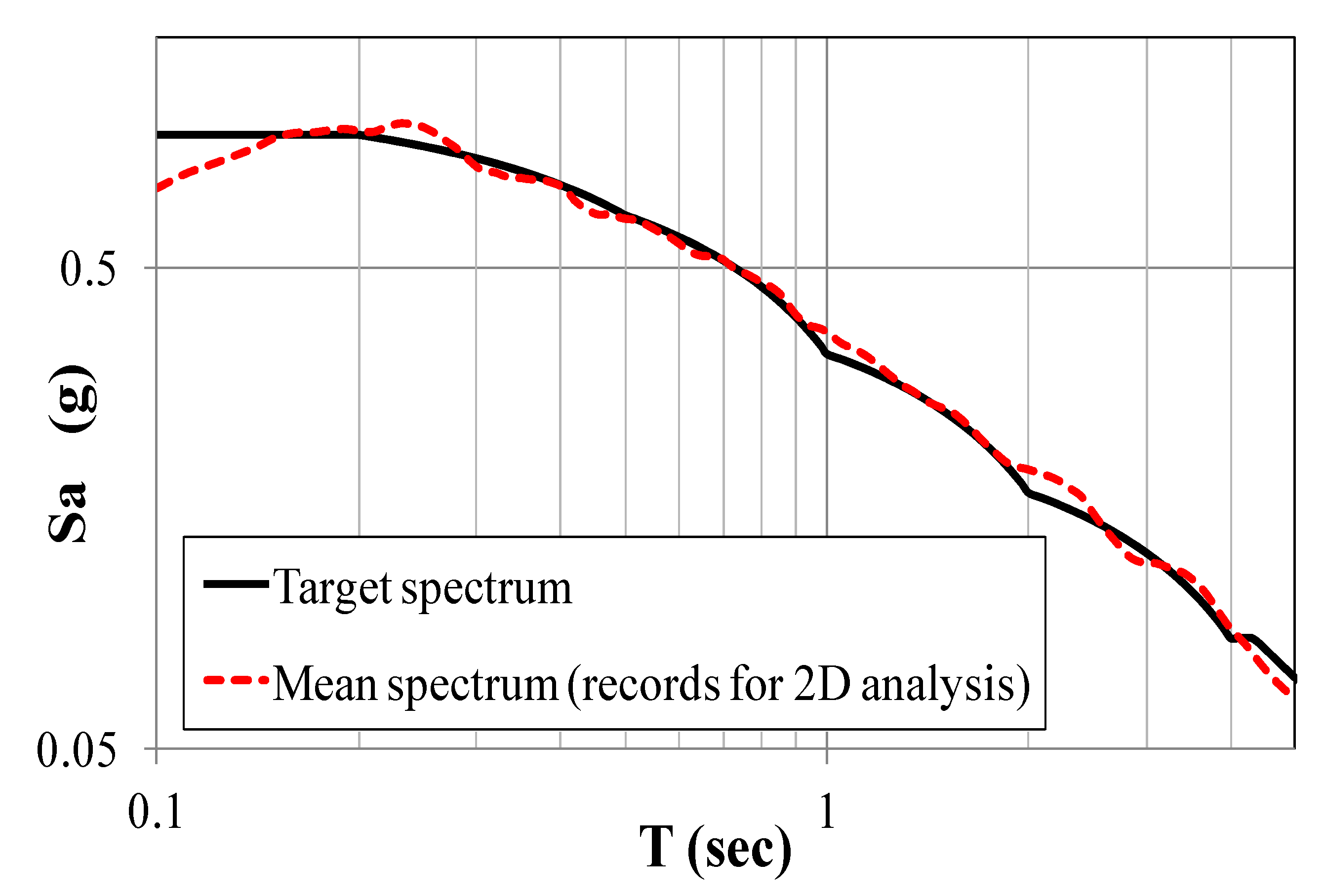
For the 3D time history analyses, the pairs of ground motion records were applied simultaneously in the longitudinal and transverse directions. However, for the 2D nonlinear analysis the horizontal components of the ground motion records are applied separately in the longitudinal and transverse directions and the seismic responses in the principal directions are treated independently, as suggested by some researchers (e.g., Priestley et al. [1]). Therefore, the average response spectral values of the horizontal components should match the design spectrum over the period range of 0.2T to 3T. It is noted that to determine the lower limit of 0.2T, the minimum of TT and TL was used, while for the upper limit of 3T the maximum of TT and TL was used. However, for 3D analyses the SRSS spectra of the 22 pairs of records were matched to 1.3 times the design spectrum and therefore it is inappropriate to use the horizontal components of these pairs for the 2D analysis. Therefore, a different set of records were selected to perform the 2D analyses. The average response spectrum of the records used for 2D analyses is shown in Figure 8 in log-log scale for the case of the regular bridge.
For the 2D analyses the bridges were subjected to 44 horizontal components of the ground motions in the transverse and longitudinal directions separately. The average displacements of the bridge columns in the transverse and longitudinal directions are summarized in Table 3 for the regular and irregular bridges. The average displacements in each of the transverse and longitudinal directions were determined using both the average of the maximum absolute displacements and the average of the maximum displacements in different directions. (positive and negative displacements). The differences between the different averaging methods were relatively small (e.g., around 10 to 20%) compared with the 3D analysis that includes displacements in the radial directions.
The displacement envelopes in the transverse direction determined using the inelastic time history and elastic response spectrum analyses are compared in Figure 9a,b for the cases of the regular and irregular bridges, respectively. While the use of the elastic analysis underestimated the seismic demands in the central column of the irregular bridge, it resulted in similar predictions for the case of the regular bridge, compared to the results obtained from the inelastic analysis. The difference between the results from linear and nonlinear analysis for the irregular bridge is mainly due to issues such as irregularity in stiffness of columns, sequential yielding of bridge columns and concentration of seismic demands in the stiffer middle column. Further details in this regard are available in Tehrani and Mitchell [52] and Tehrani [50].
Priestley et al. [1] proposed a displacement-based design concept that can be used to alleviate the problems discussed in irregular bridges. A comparison of the seismic behavior of irregular bridges designed using the force-based and displacement-based approach in CHBDC 2014 [60] indicated that seismic demands in the short columns of irregular bridges can be reduced and more uniform seismic demands can be achieved in different columns, when displacement-based design approach is used for irregular bridges [61].
The 30% rule was used to predict the maximum displacement of the bridge columns. The results indicate that the use of the 30% rule for the bridges studied resulted in very good predictions of the maximum radial displacements obtained from 3D analyses. For example, the displacements for the central columns of the regular and irregular bridges were predicted as 123 and 178 mm (Table 3), respectively, which are similar to the predictions of the radial displacements of 123 and 166 mm from 3D analyses (see Table 2). The values in the tables are for the 30% rule applied to the mean predicted displacements. It is interesting to note that when the 30% rule is applied to the results of each record individually and then the mean value is computed for the 44 different cases, then the displacements for the central columns of the regular and irregular bridges were determined as 131 and 181 mm, respectively, that is, more conservative than the tabular values.
7. Effects of Directivity on the Predictions of the Seismic Response
For the predictions of the seismic responses of the bridges in the previous sections the ground motion records were only applied in the principal axes of the bridges, which is customary in current seismic design practice (i.e., θ = 0, where the angle θ is defined in Figure 10). For bridges that have a significantly different behavior in the transverse and longitudinal directions, the effects of applying the ground motion records along different axes need to be examined.
To investigate the influence of applying the ground motion records at different angles, each pair of ground motion records was applied to the structural models at different angles, θ, from 0 to 180° with increments of 5°. The angle θ that gives the directivity of the input motions is shown in Figure 10. It was found that the responses of the bridges studied were similar for the angles θ and 180° + θ and therefore only θ values between 0 and 180° were considered. The variations of the predicted maximum radial displacements of the bridge columns are shown for 22 different pairs of records used in the analyses in Figure 11a,b for the regular and irregular bridges, respectively. As the angle θ changes, the predicted maximum radial displacements change. The maximum predicted response for each record occurs at a critical angle, θcr, which could be significantly different from that obtained by applying the records at θ = 0° (i.e., current practice). The variations of the predicted responses and the predicted critical angles differ for different records and they depend on the properties of both the records and the structure.
In Figure 11, the average responses for 7, 14, and 22 records are also shown for different values of θ. Despite the fact that the variation of the predicted responses from different records at different angles, θ, are relatively large, the variation of the predicted average responses at different angles is much smaller and as the number of records increases, the variations become even smaller. The parameter θ is considered as a random variable in this study and therefore different pairs of records can occur at different θ angles.
One approach is to use the maximum predicted response from each record at its corresponding critical angle to predict the average maximum response of the bridge. A summary of the results obtained for this case is presented in Table 4 and Figure 12b. However, this method is overly conservative, because it is highly unlikely that all input ground motions would occur at their critical angle. For example, the mean displacement for the central column of the irregular bridge was predicted as 235 mm when the records were applied at their critical angles, θcr. The predicted mean displacement for this case is about 42% larger than the mean displacement of 166 mm (see Table 2) predicted when the records were applied along the principal axes of the bridge. Similar results were observed for the case of the regular bridge.
One interesting point that can be noticed in Table 4. is that for the averaging method based on different directions the radial displacements predicted for the central critical columns are 100 mm and 133 mm for the regular and irregular bridges, respectively. These displacements are comparable to the maximum displacements of 109 mm and 138 mm, respectively, predicted in Table 2 for the displacements in the principal directions using the averaging method based on maximum absolute values for the same bridges. This may indicate that the use of a simple 3D analysis using the current simple averaging methods can predict the actual radial displacement including directivity effects, when the concepts of averaging in different directions are adopted.
In Figure 12 the average displacement of the critical central columns of the bridges in different directions are shown for two cases including when the records are applied only at the principal axes of the bridges (e.g., see Table 2 and Figure 12a) and when the records are applied at their critical angles, θcr (see Table 4 and Figure 12b). It is interesting to note that for the regular bridge the maximum displacements occur at about 270° while for the irregular bridge the maximum displacement occurs in a range close to 180°. This indicates that the transverse response is critical for the regular bridge and the longitudinal response is critical for the irregular bridge.
It is overly conservative to predict the seismic response deterministically by applying records at their critical angle and hence the uncertainty due to the angle θ should be considered probabilistically.
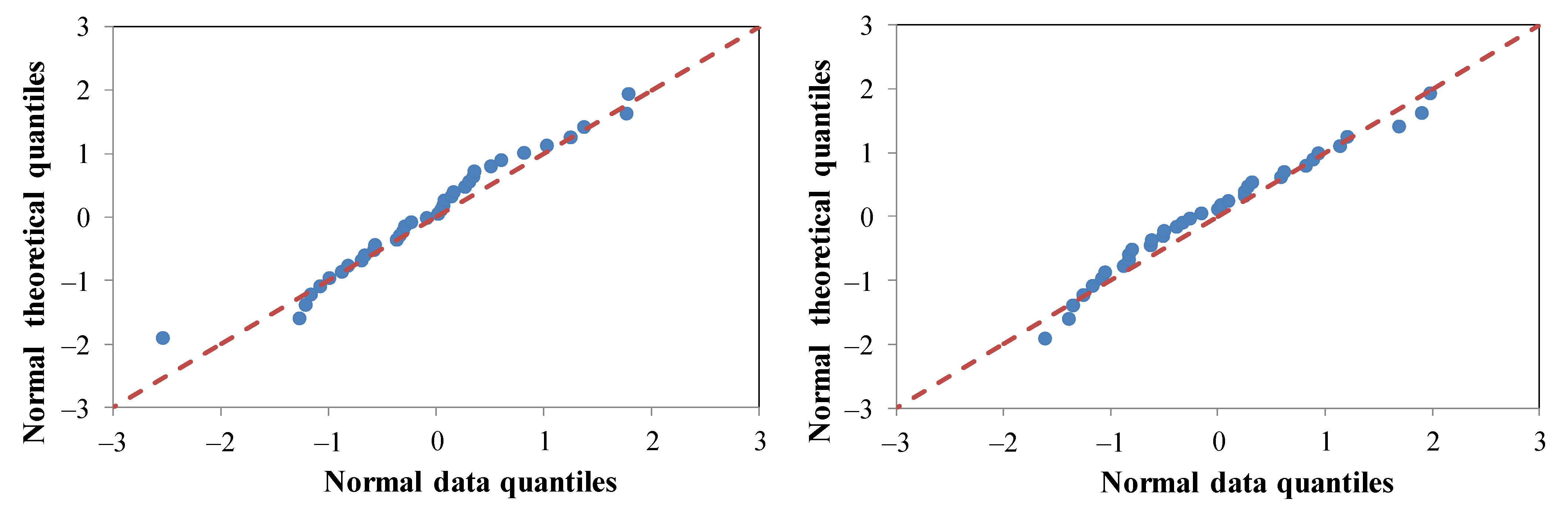
By applying each record at different θ angles a set of maximum radial displacements can be determined. For example, in this study, each record was applied at 37 different θ angles from 0° to 180° with increments of 5°. To investigate if the data is Normally distributed, the Quantile-Quantile plots (Q-Q plots) [62] were developed for the data obtained from different records. The results demonstrated that the normal distribution assumption was satisfactory. Examples of the Q-Q plots developed for two different records are shown in Figure 13.
For each record the mean and standard deviation of the maximum radial displacements, obtained by applying that record at different θ angles, can be calculated. The Normal distribution assumption can then be used to approximate the probability distribution of the maximum radial displacements at different θ angles. If n records are used in the analyses, n values of mean and standard deviation will be determined. It is well known that the average of n Normally distributed random variables is also Normally distributed with the overall mean, , and overall standard deviation, , as presented by Equations (1) and (2). As a result, the mean response of a structure subjected to n records (n ≥ 7) can be determined as a Normal random variable considering the uncertainty due to the angle θ of the records. The mean displacement of the structure subjected to a number of records can then be predicted for a certain probability of non-exceedance for design or evaluation purposes.
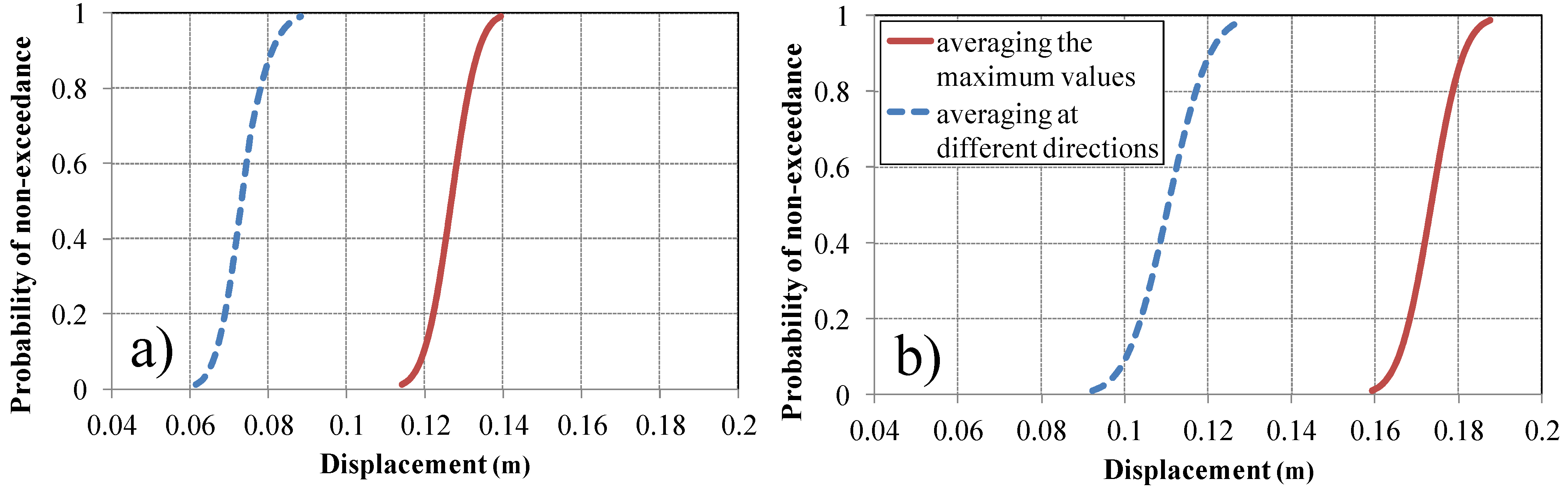
The mean and standard deviation of the maximum radial displacements of the central bridge columns are presented in Table 5 for the regular and irregular bridges studied for the same 22 records used in the previous sections of this paper. The distributions of the probability of non-exceedance for the central columns of the bridges are shown by the solid line in Figure 14.
The radial displacements of 123 and 166 mm were predicted for the central columns of the regular and irregular bridges, respectively, from 3D analyses when the ground motion records were applied in the principal directions of the bridge (see Table 2). From Figure 14 these radial displacements correspond to 10% and 25% probabilities of non-exceedance, for the regular and irregular bridges, respectively. As presented in Table 2, the use of the 30% rule resulted in predictions of 135 mm and 178 mm for the maximum displacements of the central columns of the regular and irregular bridges, respectively. These values correspond to approximately 84% probability of non-exceedance. This indicates that the use of 30% rule can reasonably account for the variability of seismic response due to different excitation angles.
It should be noted that only the variability due to the incident angle θ in the prediction of the mean response is the subject of this study. The other sources of variability, such as the record-to-record variability, are out of the scope of this study.
8. Averaging at Different Radial Directions Considering the Incident Angles, θ
The effects of variation of angle θ on the mean response of the bridge columns using the averaging procedure in different radial directions are also investigated.
A similar method as used for the case of the averaging method using the maximum absolute displacements, as previously described, can be used to predict the mean response of the bridges at different radial directions (from 0 to 360°). For this case the maximum responses are determined in m different radial directions (i.e., m = 37 radial directions with intervals of 10 ° from 0 to 360°). Assuming that the data are Normally distributed, for each record there are m values of mean and standard deviation due to the variability of angle θ along m sets of directions. The angle θ in this study ranged from 0 to 180° with increments of 5° (i.e., 37 different angles). Therefore, the mean and standard deviation of the data, due to variation of angle θ, from record i in direction j can be determined as Mij and Sij, respectively. Therefore, with reference to Equations (1) and (2), the mean and standard deviation of the average response in each direction j, M′j and S′j, then can be estimated using Equations (3) and (4), by averaging the results from n ground motion records in each direction. The maximum value of the m Normal random variables with a mean and standard deviation of M′j and S′j can then be determined to predict the critical displacement. The probability distribution of the maximum displacement in the different directions can be predicted numerically by computing the maximum displacement within m random variables at different probabilities of non-exceedance. The predicted probability distributions of the displacements of the central column are shown by dashed line in Figure 14 for the regular and irregular bridges.
For example, the predicted displacements of 84 and 114 mm for the central columns of the regular and irregular bridges, when the angle θ was not considered (see Table 2), corresponds to 95% and 70% probabilities of non-exceedance, respectively (see Figure 14).
It should be noted that the Performance-Based Design (PBD) concepts have been introduced in the 2014 edition of the Canadian Highway Bridge Design Code (CHBDC) [60].
The subjects studied in this research can be also investigated for bridges designed based on the new design concepts of 2014 CHBDC. For example, the effects of directivity on the maximum strains in the steel and concrete considering different displacement directions can be studied and be compared to the strain limitations given in 2014 CHBDC. Some researchers such as Zhang et al. [63] have concluded that the strain limitations in 2014 CHBDC are conservative. More research is needed on this subject.
9. Conclusions
This study, while limited to two bridges, demonstrates that the influence of the directivity of ground motion is important and guidance is given on predicting the mean response considering the effects of directivity of horizontal ground motions. Conclusions from this study are summarized as follows:
(1) The use of the 30% rule using 2D analyses resulted in good predictions of the maximum radial displacement of columns for the case of the straight bridges studied in this research, when the average displacements were computed using the maximum absolute displacements for each ground motion record. No general conclusion can be made in this regard without further research.
(2) When the averaging procedure involving the prediction of the mean displacements in different radial directions was adopted for the bridges in this study, the maximum radial displacements obtained using 3D analyses were smaller than the maximum displacements obtained in the longitudinal and transverse directions using 2D analysis. However, when the averaging procedure based on the maximum absolute values was adopted to determine the mean displacements, the displacements in the transverse and longitudinal directions needed to be combined using the 30% rule resulting in predictions similar to those obtained using 3D analyses.
(3) The use of the averaging method in different radial directions, which is more logical than the averaging methods using the maximum absolute displacements, resulted in 40–50% smaller predicted displacements for the 3D analyses. For this approach the maximum possible mean radial displacements predicted, that is, when all records were applied at their critical angles at the same time, was in the order of the maximum response predicted in the principal axes for a 3D analysis using absolute maximum values and without considering the directivity effects (i.e., simple method that typically used in practice). This means that when the concepts of averaging in different directions is adopted, the use of a simple 3D analysis without considering directivity effects and without determining the radial displacements may predict the maximum response, when averaging based on maximum absolute values are used only for the displacements along the principal axes of the bridge.
(4) By comparing the seismic response of the regular and irregular bridges predicted using different approaches, it was observed that for the irregular bridge significantly larger ductility demands and plastic rotations occur in the shortest column compared to the case of the regular bridge. This can significantly affect the vulnerability of the irregular bridges.
(5) When all of the records were applied at their critical angles (overly conservative case), the predicted displacements increased by 40–50% compared to the predictions determined by applying the records in the principal axes of the structure.
(6) A method was proposed to predict the variability in the mean response due to the application of the pairs of records at different angles θ. Although the response of the individual records was found to be sensitive to the variations of angle θ, when the mean response was considered the variations were relatively small.
(7) Although the use of the 30% rule provides conservative predictions of the radial displacements when compared with the predictions using 3D analyses, when directivity effects are not considered, this conservatism allows for some increases in the radial displacements due to different excitation angles, θ. The probability of exceeding the mean radial displacements of the columns, obtained from the 30% rule, was about 15 to 20%, for the cases studied when directionality effects were considered. This probability may be higher for different structures especially some highly irregular structures. More research is needed on this subject.
(8) The combination rules such as 100–30% rule in the codes are typically recommended and used for the elastic analysis methods, when a bridge is designed. It is not clear if the use of such combination rules are also intended, by the codes, for inelastic time history analyses. While directivity effects are considered in some new codes by requiring that the records be applied at random directions, displacements along the principal axes of the bridge (e.g., X and Y directions) are used for design and evaluation. It was shown that the actual maximum radial displacement occurred in a random direction and was around 15 to 20% larger than that in the principal axes directions. When directivity effects were considered in the analysis, the difference can increase up to 70% (i.e., when all records were applied at their critical angles). Therefore, the use of the combination rules may under predict the maximum displacements, when both directivity effects of records and radial displacement of columns are considered. More research is needed.
Author Contributions
Conceptualization, P.T. and D.M.; methodology, P.T.; software, P.T.; validation, P.T.; investigation, P.T.; resources, P.T. and D.M.; data curation, P.T.; writing—original draft preparation, P.T.; writing—review and editing, P.T. and D.M.; visualization, P.T.; supervision, D.M.; project administration, D.M.; funding acquisition, D.M. All authors have read and agreed to the published version of the manuscript.
Funding
This research received no external funding.
Institutional Review Board Statement
Not applicable.
Informed Consent Statement
Not Applicable.
Data Availability Statement
The data presented in this study are available on request from the corresponding author.
Acknowledgments
Simulated ground motion records developed by Atkinson (2009) were obtained from www.seismotoolbox.ca. (accessed in March 2014). Natural ground motion data obtained from the PEER-NGA database is available at http://peer.berkeley.edu (accessed in March 2014).
Conflicts of Interest
The authors declare no conflict of interest.
References
- Priestley, M.J.N.; Calvi, G.M.; Kowalsky, M.J. Displacement-Based Seismic Design of Structures; IUSS Press: Pavia, Italy, 2007. [Google Scholar]
- Caltrans, C. Seismic Design Criteria (SDC); version 2.0; California Department of Transportation: Sacramento, CA, USA, 2019.
- AASHTO. AASHTO Guide Specifications for LRFD Seismic Bridge Design; AASHTO: Washington, DC, USA, 2011. [Google Scholar]
- Penzien, J.; Watabe, M. Characteristics of 3-dimensional earthquake ground motions. Earthq. Eng. Struct. Dyn. 1974, 3, 365–373. [Google Scholar] [CrossRef]
- López, O.A.; Torres, R. The critical angle of seismic incidence and the maximum structural response. Earthq. Eng. Struct. Dyn. 1997, 26, 881–894. [Google Scholar] [CrossRef]
- Menun, C.; Der Kiureghian, A. A replacement for the 30%, 40%, and SRSS rules for multicomponent seismic analysis. Earthq. Spectra 1998, 14, 153–163. [Google Scholar] [CrossRef]
- Lopez, O.A.; Chopra, A.K.; Hernandez, J.J. Critical response of structures to multicomponent earthquake excitation. Earthq. Eng. Struct. Dyn. 2000, 29, 1759–1778. [Google Scholar] [CrossRef]
- Anastassiadis, K.; Avramidis, I.E.; Panetsos, P. Concurrent design forces in structures under three-component orthotropic seismic excitation. Earthq. Spectra 2002, 18, 1–17. [Google Scholar] [CrossRef]
- Athanatopoulou, A. Critical orientation of three correlated seismic components. Eng. Struct. 2005, 27, 301–312. [Google Scholar] [CrossRef]
- Rigato, A.B.; Medina, R.A. Influence of angle of incidence on seismic demands for inelastic single-storey structures subjected to bi-directional ground motions. Eng. Struct. 2007, 29, 2593–2601. [Google Scholar] [CrossRef]
- Maleki, S.; Bisadi, V. Orthogonal effects in seismic analysis of skewed bridges. J. Bridge Eng. 2006, 11, 122–130. [Google Scholar] [CrossRef]
- Bisadi, V.; Head, M. Orthogonal effects in nonlinear analysis of bridges subjected to multicomponent earthquake excitation. In Proceedings of the Structures Congress 2010, Orlando, FL, USA, 12–15 May 2010; American Society of Civil Engineers: Reston, VA, USA, 2010. [Google Scholar]
- Moschonas, I.F.; Kappos, A.J. Assessment of concrete bridges subjected to ground motion with an arbitrary angle of incidence: Static and dynamic approach. Bull. Earthq. Eng. 2013, 11, 581–605. [Google Scholar] [CrossRef] [Green Version]
- Bisadi, V.; Head, M. Evaluation of combination rules for orthogonal seismic demands in nonlinear time history analysis of bridges. J. Bridge Eng. 2011, 16, 711–717. [Google Scholar] [CrossRef]
- Khaled, A.; Tremblay, R.; Massicotte, B. Effectiveness of the 30%-rule at predicting the elastic seismic demand on bridge columns subjected to bi-directional earthquake motions. Eng. Struct. 2011, 33, 2357–2370. [Google Scholar] [CrossRef]
- Khaled, A.; Tremblay, R.; Massicotte, B. Combination rule for the prediction of the seismic demand on columns of regular bridges under bidirectional earthquake components. Can. J. Civ. Eng. 2011, 38, 698–709. [Google Scholar] [CrossRef]
- Mackie, K.R.; Cronin, K.J.; Nielson, B.G. Response sensitivity of highway bridges to randomly oriented multi-component earthquake excitation. J. Earthq. Eng. 2011, 15, 850–876. [Google Scholar] [CrossRef]
- Banerjee Basu, S.; Shinozuka, M. Effect of ground motion directionality on fragility characteristics of a highway bridge. Adv. Civ. Eng. 2011, 2011, 536171. [Google Scholar] [CrossRef] [Green Version]
- Torbol, M.; Shinozuka, M. Effect of the angle of seismic incidence on the fragility curves of bridges. Earthq. Eng. Struct. Dyn. 2012, 41, 2111–2124. [Google Scholar] [CrossRef]
- Torbol, M.; Shinozuka, M. The directionality effect in the seismic risk assessment of highway networks. Struct. Infrastruct. Eng. 2014, 10, 175–188. [Google Scholar] [CrossRef]
- Taskari, O.; Sextos, A. Multi-angle, multi-damage fragility curves for seismic assessment of bridges. Earthq. Eng. Struct. Dyn. 2015, 44, 2281–2301. [Google Scholar] [CrossRef]
- Emami, A.R.; Halabian, A.M. Spatial distribution of ductility demand and damage index in 3D RC frame structures considering directionality effects. Struct. Des. Tall Spec. Build. 2015, 24, 941–961. [Google Scholar] [CrossRef]
- Bhatnagar, U.R.; Banerjee, S. Fragility of skewed bridges under orthogonal seismic ground motions. Struct. Infrastruct. Eng. 2015, 11, 1113–1130. [Google Scholar] [CrossRef]
- Bayat, M.; Daneshjoo, F.; Nisticò, N. The effect of different intensity measures and earthquake directions on the seismic assessment of skewed highway bridges. Earthq. Eng. Eng. Vib. 2017, 16, 165–179. [Google Scholar] [CrossRef]
- Omranian, E.; Abdelnaby, A.E.; Abdollahzadeh, G. Seismic vulnerability assessment of RC skew bridges subjected to mainshock-aftershock sequences. Soil Dyn. Earthq. Eng. 2018, 114, 186–197. [Google Scholar] [CrossRef]
- Feng, R.; Wang, X.; Yuan, W.; Yu, J. Impact of seismic excitation direction on the fragility analysis of horizontally curved concrete bridges. Bull. Earthq. Eng. 2018, 16, 4705–4733. [Google Scholar] [CrossRef]
- Soltanieh, S.; Memarpour, M.M.; Kilanehei, F. Performance assessment of bridge-soil-foundation system with irregular configuration considering ground motion directionality effects. Soil Dyn. Earthq. Eng. 2019, 118, 19–34. [Google Scholar] [CrossRef]
- Noori, H.; Memarpour, M.M.; Yakhchalian, M.; Soltanieh, S. Effects of ground motion directionality on seismic behavior of skewed bridges considering SSI. Soil Dyn. Earthq. Eng. 2019, 127, 105820. [Google Scholar] [CrossRef]
- Shan, D.; Qu, F.; Deng, X. Seismic fragility analysis of irregular bridges with non-circular tall piers considering ground motion directionality. Bull. Earthq. Eng. 2020, 18, 1723–1753. [Google Scholar] [CrossRef]
- D’Amato, M.; Laguardia, R.; Di Trocchio, G.; Coltellacci, M.; Gigliotti, R. Seismic Risk Assessment for Masonry Buildings Typologies from L’Aquila 2009 Earthquake Damage Data. J. Earthq. Eng. 2020, 1–35. [Google Scholar] [CrossRef]
- American Society of Civil Engineers. ASCE/SEI 7-16, Minimum Design Loads and Associated Criteria for Buildings and Other Structures; American Society of Civil Engineers: Reston, VA, USA, 2017. [Google Scholar]
- American Society of Civil Engineers. ASCE/SEI 41-17, Seismic Evaluation and Retrofit of Existing Buildings; American Society of Civil Engineers: Reston, VA, USA, 2017. [Google Scholar]
- Aviram, A.; Mackie, K.R.; Stojadinovic, B. Effect of abutment modeling on the seismic response of bridge structures. Earthq. Eng. Eng. Vib. 2008, 7, 395–402. [Google Scholar] [CrossRef]
- Tehrani, P.; Mitchell, D. Effects of column stiffness irregularity on the seismic response of bridges in the longitudinal direction. Can. J. Civ. Eng. 2013, 40, 815–825. [Google Scholar] [CrossRef]
- Isaković, T.; Lazaro, M.P.N.; Fischinger, M. Applicability of pushover methods for the seismic analysis of single-column bent viaducts. Earthq. Eng. Struct. Dyn. 2008, 37, 1185–1202. [Google Scholar] [CrossRef]
- Calvi, G.; Elnashai, A.; Pavese, A. Influence of regularity on the seismic response of RC bridges. In Proceedings of the 2nd International Workshop on Seismic Design and Retrofitting of RC Bridges, Queenstown, New Zealand, 8–13 August 1994. [Google Scholar]
- Akbari, R. Seismic fragility analysis of reinforced concrete continuous span bridges with irregular configuration. Struct. Infrastruct. Eng. 2012, 8, 873–889. [Google Scholar] [CrossRef]
- Bardakis, V.G.; Fardis, M.N. Nonlinear dynamic v elastic analysis for seismic deformation demands in concrete bridges having deck integral with the piers. Bull. Earthq. Eng. 2011, 9, 519–535. [Google Scholar] [CrossRef]
- Tehrani, P.; Mitchell, D. Seismic risk assessment of four-span bridges in Montreal designed using the Canadian bridge design code. J. Bridge Eng. 2014, 19, A4014002. [Google Scholar] [CrossRef]
- Tehrani, P.; Mitchell, D. Seismic response of bridges subjected to different earthquake types using IDA. J. Earthq. Eng. 2013, 17, 423–448. [Google Scholar] [CrossRef]
- Canadian Standards Association. CAN/CSA-S6-10. Canadian Highway Bridge Design Code (CHBDC) and Commentary; Canadian Standards Association: Mississauga, ON, USA, 2010. [Google Scholar]
- National Research Council of Canada. National Building Code of Canada (NBCC); National Research Council of Canada: Ottawa, ON, Canada, 2010.
- Berry, M.P.; Eberhard, M.O. Performance Modeling Strategies for Modern Reinforced Concrete Bridge Columns; University of California: Berkeley, CA, USA, 2006; Volume 67. [Google Scholar]
- Otani, S. Hysteresis models of reinforced concrete for earthquake response analysis. J. Fac. Eng. 1981, 36, 125–159. [Google Scholar]
- Carr, A. RUAUMOKO, a Computer Program for Inelastic Dynamic Analysis; Department of Civil Engineering, University of Canterbury: Christchurch, New Zealand, 2009. [Google Scholar]
- Tehrani, P.; Mitchell, D. Seismic performance assessment of bridges in Montreal using incremental dynamic analysis. In Proceedings of the 15th World Conference on Earthquake Engineering, Lisbon, Portugal, 24–28 September 2012. [Google Scholar]
- Priestley, M.J.N.; Seible, F.; Calvi, G.M. Seismic Design and Retrofit of Bridges; John Wiley & Sons: Hoboken, NJ, USA, 1996. [Google Scholar]
- Priestley, M.N.; Benzoni, G. Seismic performance of circular columns with low longitudinal reinforcement ratios. Struct. J. 1996, 93, 474–485. [Google Scholar]
- Berry, M.; Parrish, M.; Eberhard, M. PEER Structural Performance Database User’s Manual; University of California: Berkeley, CA, USA, 2004. [Google Scholar]
- Tehrani, P. Seismic Behaviour and Analysis of Continuous Reinforced Concrete Bridges. Ph.D. Thesis, McGill University Libraries, Montréal, QC, Canada, 2012. [Google Scholar]
- Pinto, A.; Verzeletti, G.; Magonette, G.; Pegon, P.; Negro, P.; Guedes, J. Pseudo-dynamic testing of large-scale R/C bridges in ELSA. In Proceedings of the 11th World Conference on Earthquake Engineering, Acapulco, Mexico, 23–28 June 1996. [Google Scholar]
- Tehrani, P.; Mitchell, D. Effects of column and superstructure stiffness on the seismic response of bridges in the transverse direction. Can. J. Civ. Eng. 2013, 40, 827–839. [Google Scholar] [CrossRef]
- Tehrani, P.; Mitchell, D. Investigating the Use of Natural and Artificial Records for Prediction of Seismic Response of Regular and Irregular RC Bridges Considering Displacement Directions. Appl. Sci. 2021, 11, 906. [Google Scholar] [CrossRef]
- Stewart, J.P.; Abrahamson, N.A.; Atkinson, G.M.; Baker, J.W.; Boore, D.M.; Bozorgnia, Y.; Campbell, K.W.; Comartin, C.D.; Idriss, I.M.; Lew, M.; et al. Representation of bidirectional ground motions for design spectra in building codes. Earthq. Spectra 2011, 27, 927–937. [Google Scholar] [CrossRef]
- American Society of Civil Engineers. ASCE/SEI 7-10, Minimum Design Loads for Buildings and Other Structures; American Society of Civil Engineers: Reston, VA, USA, 2010. [Google Scholar]
- American Society of Civil Engineers. ASCE/SEI 7-05, Minimum Design Loads for Buildings and Other Structures; American Society of Civil Engineers: Reston, VA, USA, 2005. [Google Scholar]
- Tehrani, P.; Goda, K.; Mitchell, D.; Atkinson, G.M.; Chouinard, L.E. Effects of different record selection methods on the seismic response of bridges in South Western Brihish Colombia. J. Earthq. Eng. 2014, 18, 611–636. [Google Scholar] [CrossRef]
- Baker, J.W. Conditional mean spectrum: Tool for ground-motion selection. J. Struct. Eng. 2011, 137, 322–331. [Google Scholar] [CrossRef]
- NIST GCR. GCR 11-917-15: Selecting and Scaling Earthquake Ground Motions for Performing Response-History Analyses; National Institute of Standards and Technology, US Department of Commerce: Gaithersburg, MD, USA, 2011.
- CSA. Canadian Highway Bridge Design Code; CSA: Toronto, ON, Canada, 2014. [Google Scholar]
- Reza, S.M.; Alam, M.S.; Tesfamariam, S. Seismic performance comparison between direct displacement-based and force-based design of a multi-span continuous reinforced concrete bridge with irregular column heights. Can. J. Civ. Eng. 2014, 41, 440–449. [Google Scholar] [CrossRef]
- Wilk, M.B.; Gnanadesikan, R. Probability plotting methods for the analysis for the analysis of data. Biometrika 1968, 55, 1–17. [Google Scholar] [CrossRef] [PubMed]
- Zhang, Q.; Alam, M.S.; Khan, S.; Jiang, J. Seismic performance comparison between force-based and performance-based design as per Canadian Highway Bridge Design Code (CHBDC) 2014. Can. J. Civ. Eng. 2016, 43, 741–748. [Google Scholar] [CrossRef] [Green Version]
Figure 1.
Outline of the study including steps taken and procedure used.

Figure 2.
Bridges properties: (a) regular bridge; (b) irregular bridge.

Figure 3.
Structural modelling of the bridges: (a) Schematic presentation of the structural modelling of the bridge in the RUAUMOKO program (adapted from [34]) (b) Modified Takeda hysteresis loop (adapted from [45]).

Figure 4.
Comparison of the experimental data for the short column of the bridge B213C tested by Pinto et al. [51] and results from numerical analysis: (a) column displacement for the maximum earthquake and (b) cyclic response of the column.
Figure 4.
Comparison of the experimental data for the short column of the bridge B213C tested by Pinto et al. [51] and results from numerical analysis: (a) column displacement for the maximum earthquake and (b) cyclic response of the column.

Figure 5.
SRSS response spectra and mean SRSS spectrum of 22 records used for the analysis of: (a) regular bridge; (b) irregular bridge.
Figure 5.
SRSS response spectra and mean SRSS spectrum of 22 records used for the analysis of: (a) regular bridge; (b) irregular bridge.

Figure 6.
An example of the time history results for the longitudinal, transverse and radial displacements.
Figure 6.
An example of the time history results for the longitudinal, transverse and radial displacements.

Figure 7.
The maximum displacements obtained from 22 records using the maximum absolute displacements for: (a) regular bridge; (b) irregular bridge; and using the negative and positive displacements for: (c) regular bridge; (d) irregular bridge.
Figure 7.
The maximum displacements obtained from 22 records using the maximum absolute displacements for: (a) regular bridge; (b) irregular bridge; and using the negative and positive displacements for: (c) regular bridge; (d) irregular bridge.

Figure 8.
Mean response spectra of 44 horizontal components of the ground motion records selected for 2D analysis (target spectrum for Vancouver, site class C).
Figure 8.
Mean response spectra of 44 horizontal components of the ground motion records selected for 2D analysis (target spectrum for Vancouver, site class C).

Figure 9.
Transverse displacement envelopes obtained by means of 2D elastic and inelastic analyses for: (a) regular bridge (b) irregular bridge.
Figure 9.
Transverse displacement envelopes obtained by means of 2D elastic and inelastic analyses for: (a) regular bridge (b) irregular bridge.

Figure 10.
Applying two horizontal components of the records, H1 and H2, along X′ and Y′ axes rotated by θ° relative to the principal axes of structure, X (longitudinal direction) and Y (transverse direction).
Figure 10.
Applying two horizontal components of the records, H1 and H2, along X′ and Y′ axes rotated by θ° relative to the principal axes of structure, X (longitudinal direction) and Y (transverse direction).

Figure 11.
Maximum radial displacement of the critical central column for different records applied at different angles θ for (a) regular bridge; (b) irregular bridge.
Figure 11.
Maximum radial displacement of the critical central column for different records applied at different angles θ for (a) regular bridge; (b) irregular bridge.

Figure 12.
Mean displacement of the central column of the bridges along different directions for: (a) records applied along the principal axes of bridges; (b) records applied at their critical angle, θcr.
Figure 12.
Mean displacement of the central column of the bridges along different directions for: (a) records applied along the principal axes of bridges; (b) records applied at their critical angle, θcr.

Figure 13.
Examples of Normal Quantile-Quantile plots for two different records.

Figure 14.
Probability of non-exceedance for the mean displacements of the central column using different averaging methods, due to variability of angle θ, for: (a) regular bridge; (b) irregular bridge.
Figure 14.
Probability of non-exceedance for the mean displacements of the central column using different averaging methods, due to variability of angle θ, for: (a) regular bridge; (b) irregular bridge.


Table 1.
Modal properties of bridges including periods and (effective modal mass ratios).
| TT1 (sec) | TT2 (sec) | TL (sec) | TG (sec) | |
|---|---|---|---|---|
| Regular bridge | 0.75 (87%) | 0.28 (8%) | 0.90 (100%) | 0.82 |
| Irregular bridge | 0.93 (90%) | 0.29 (5%) | 1.28 (100%) | 1.09 |
Table 2.
Summary of the mean displacements (mm) of columns using 3D analysis for the regular and irregular bridges with mean ductility demands given in brackets.
Table 2.
Summary of the mean displacements (mm) of columns using 3D analysis for the regular and irregular bridges with mean ductility demands given in brackets.
| Regular Bridge | Irregular Bridge | ||||
|---|---|---|---|---|---|
| Average of Absolute Maximum Values | Average in Different Directions | Average of Absolute Maximum Values | Average in Different Directions | ||
| Transverse | Column 1 | 77 (2.0) | 64 (1.7) | 95 (0.66) | 82 (0.6) |
| Column 2 | 109 (2.8) | 93 (2.4) | 131 (3.24) | 112 (2.8) | |
| Column 3 | 77 (2.0) | 65 (1.7) | 101 (0.32) | 88 (0.3) | |
| Longitudinal | Columns 1, 2 and 3 | 86 (2.2) | 74 (1.9) | 138 (1.0, 3.4, 0.4) | 124 (0.9, 3.1, 0.4) |
| Radial | Column 1 | 101 (2.6) | 69 (1.8) | 148 (1.0) | 116 (0.8) |
| Column 2 | 123 (3.2) | 84 (2.2) | 166 (4.1) | 114 (2.8) | |
| Column 3 | 100 (2.6) | 69 (1.8) | 151 (0.5) | 115 (0.4) | |
| 30% Rule | Column 1 | 109 (2.8) | 94 (2.4) | 167 (1.2) | 149 (1.0) |
| Column 2 | 135 (3.5) | 116 (3.0) | 178 (4.4) | 158 (3.9) | |
| Column 3 | 109 (2.8) | 94 (2.4) | 169 (0.5) | 151 (0.5) | |
Table 3.
Summary of the mean displacements (mm) of columns using 2D analysis for the regular and irregular bridges with mean ductility demands given in brackets.
Table 3.
Summary of the mean displacements (mm) of columns using 2D analysis for the regular and irregular bridges with mean ductility demands given in brackets.
| Regular Bridge | Irregular Bridge | ||||
|---|---|---|---|---|---|
| Average of Absolute Maximum Values | Average in Different Directions | Average of Absolute Maximum Values | Average in Different Directions | ||
| Transverse | Column 1 | 64 (1.7) | 58 (1.5) | 78 (0.6) | 69 (0.5) |
| Column 2 | 94 (2.4) | 84 (2.2) | 110 (2.7) | 96 (2.4) | |
| Column 3 | 64 (1.7) | 58 (1.5) | 86 (0.3) | 76 (0.2) | |
| Longitudinal | Columns 1, 2 and 3 | 96 (2.5) | 81 (2.1) | 145 (1.0, 3.6, 0.5) | 130 (0.9, 3.2, 0.4) |
| 30% Rule | Column 1 | 115 (3.0) | 98 (2.6) | 169 (1.2) | 151(1.1) |
| Column 2 | 123 (3.2) | 109 (2.8) | 178 (4.4) | 158 (3.9) | |
| Column 3 | 115 (3.0) | 98 (2.6) | 171 (0.5) | 153 (0.5) | |
Table 4.
Summary of the mean displacements (mm) of columns using 3D analysis for the regular and irregular bridges by applying the records at their critical angle (i.e., maximum possible seismic demands). Mean ductility demands given in brackets.
Table 4.
Summary of the mean displacements (mm) of columns using 3D analysis for the regular and irregular bridges by applying the records at their critical angle (i.e., maximum possible seismic demands). Mean ductility demands given in brackets.
| Regular Bridge | Irregular Bridge | ||||
|---|---|---|---|---|---|
| Average of Absolute Maximum Values | Average in Different Directions | Average of Absolute Maximum Values | Average in Different Directions | ||
| Transverse | Column 1 | 81 (2.1) | 71 (1.8) | 88 (0.6) | 76 (0.5) |
| Column 2 | 156 (4.0) | 129 (3.4) | 147 (3.6) | 126 (3.1) | |
| Column 3 | 81 (2.1) | 71 (1.8) | 98 (0.3) | 84 (0.3) | |
| Longitudinal | Columns 1, 2 and 3 | 133 (3.5) | 105 (2.7) | 196 (1.4, 4.9, 0.7) | 159 (1.1, 3.9, 0.6) |
| Radial | Column 1 | 148 (3.9) | 93 (2.4) | 220 (1.5) | 143 (1.0) |
| Column 2 | 175 (4.5) | 100 (2.6) | 235 (5.8) | 133 (3.3) | |
| Column 3 | 148 (3.8) | 90 (2.3) | 221 (0.7) | 142 (0.5) | |
| 30% Rule | Column 1 | 157 (4.1) | 127 (3.3) | 222 (1.6) | 190 (1.3) |
| Column 2 | 180 (4.7) | 154 (4.0) | 240 (5.9) | 197 (4.9) | |
| Column 3 | 157 (4.1) | 125 (3.2) | 225 (0.7) | 191 (0.6) | |
Table 5.
Mean and standard deviation of the central column displacements (mm) for different records applied at different angles, θ.
Table 5.
Mean and standard deviation of the central column displacements (mm) for different records applied at different angles, θ.
| Regular Bridge | Irregular Bridge | ||||||||||
|---|---|---|---|---|---|---|---|---|---|---|---|
| Record No. | Mean | St Dev | Record No. | Mean | St Dev | Record No. | Mean | St Dev | Record No. | Mean | St Dev |
| 1 | 113.4 | 10.8 | 12 | 118.5 | 15.8 | 1 | 159.9 | 12.6 | 12 | 144.1 | 16.1 |
| 2 | 152.8 | 26.9 | 13 | 114.0 | 18.3 | 2 | 155.9 | 17.4 | 13 | 203.8 | 31.3 |
| 3 | 131.0 | 10.7 | 14 | 121.6 | 9.5 | 3 | 166.8 | 13.7 | 14 | 173.2 | 25.3 |
| 4 | 154.3 | 35.4 | 15 | 151.4 | 41.2 | 4 | 188.4 | 40.0 | 15 | 154.6 | 25.3 |
| 5 | 95.7 | 17.7 | 16 | 117.1 | 19.7 | 5 | 224.4 | 26.1 | 16 | 127.0 | 13.5 |
| 6 | 152.1 | 26.9 | 17 | 109.1 | 11.3 | 6 | 144.8 | 26.1 | 17 | 184.5 | 48.3 |
| 7 | 168.0 | 31.6 | 18 | 134.9 | 23.5 | 7 | 170.9 | 34.6 | 18 | 168.4 | 36.9 |
| 8 | 112.5 | 10.1 | 19 | 90.7 | 12.0 | 8 | 141.4 | 16.9 | 19 | 133.8 | 20.8 |
| 9 | 137.9 | 21.3 | 20 | 131.3 | 37.8 | 9 | 229.0 | 33.2 | 20 | 194.5 | 28.4 |
| 10 | 129.8 | 15.8 | 21 | 123.0 | 56.5 | 10 | 197.7 | 30.0 | 21 | 135.1 | 11.4 |
| 11 | 123.8 | 22.3 | 22 | 106.1 | 16.6 | 11 | 209.7 | 42.3 | 22 | 206.9 | 37.7 |
| Overall | = 126.7 | = 5.4 | Overall | = 173.4 | = 6.1 | ||||||
Publisher’s Note: MDPI stays neutral with regard to jurisdictional claims in published maps and institutional affiliations. |
© 2021 by the authors. Licensee MDPI, Basel, Switzerland. This article is an open access article distributed under the terms and conditions of the Creative Commons Attribution (CC BY) license (http://creativecommons.org/licenses/by/4.0/).
Share and Cite
MDPI and ACS Style
Tehrani, P.; Mitchell, D. Prediction of Mean Responses of RC Bridges Considering the Incident Angle of Ground Motions and Displacement Directions. Appl. Sci. 2021, 11, 2462. https://0-doi-org.brum.beds.ac.uk/10.3390/app11062462
AMA Style
Tehrani P, Mitchell D. Prediction of Mean Responses of RC Bridges Considering the Incident Angle of Ground Motions and Displacement Directions. Applied Sciences. 2021; 11(6):2462. https://0-doi-org.brum.beds.ac.uk/10.3390/app11062462
Chicago/Turabian StyleTehrani, Payam, and Denis Mitchell. 2021. "Prediction of Mean Responses of RC Bridges Considering the Incident Angle of Ground Motions and Displacement Directions" Applied Sciences 11, no. 6: 2462. https://0-doi-org.brum.beds.ac.uk/10.3390/app11062462
Note that from the first issue of 2016, this journal uses article numbers instead of page numbers. See further details here.