
Shape Optimization of an Open Photoacoustic Resonator


1
Department of Mechanical Engineering and Production, Hamburg University of Applied Sciences, Berliner Tor 21, 20099 Hamburg, Germany
2
Department of Mechanical and Electrical Engineering, University of Southern Denmark, 6400 Sønderborg, Denmark
*
Author to whom correspondence should be addressed.
Appl. Sci. 2021, 11(6), 2571; https://0-doi-org.brum.beds.ac.uk/10.3390/app11062571
Submission received: 22 February 2021
/
Revised: 10 March 2021
/
Accepted: 11 March 2021
/
Published: 13 March 2021
(This article belongs to the Special Issue State-of-the-Art Laser Measurement Technologies)
Abstract
:Photoacoustic (PA) measurements with open resonators usually provide poor detection sensitivity due to signal leakage at the resonator opening. We have recently demonstrated three different approaches for modelling the photoacoustic signal of open resonators. In this work, one of the approaches is applied for the optimization of the geometry of the T-shaped resonator for improved signal strength and thus sensitivity. The results from the numerical optimization show an increase in the photoacoustic signal by a factor of approximately 7.23. They are confirmed using numerical methods other than the one applied for the optimization and by experimental measurement. The measurement shows an increase in the photoacoustic signal by a factor of approximately 2.34.
1. Introduction
Photoacoustic spectroscopy (PAS) is a technique based on the generation of an acoustic signal after the absorption of light by molecules [1]. It has been widely applied in numerous fields ranging from evaluation of materials [2,3], agriculture [4,5], medical/biological applications [6,7,8] and environmental analysis [9,10,11]. PAS offers high detection sensitivity as low as the parts per billion (ppb) level [12] and is suitable for the measurement of optically opaque samples where traditional absorption spectroscopic methods fail. Often, acoustic resonators are employed to significantly amplify the photoacoustic signal. In a conventional experimental setup the sample is located inside a sealed resonator. However, in specific applications a closed resonator is not suitable, and an open resonator configuration is required.
Photoacoustic (PA) measurements of blood glucose levels are performed using open T-shaped resonators [13,14]. One of the resonator ends is left unsealed to prevent an increase of humidity within the resonator that is caused by skin transpiration [13]. This is because PA glucose measurements are performed using mid-infrared radiation (MIR) and water has strong absorption in the MIR region. Humidity leads to increased absorption of MIR that interferes with PA glucose measurements. Furthermore, the opening helps to improve the stability of the measurement by minimizing temperature fluctuations [13]. However, the opening deteriorates the photoacoustic (PA) signal. As a consequence, the detection sensitivity is not quite sufficient for an industrial implementation of a diagnostic sensor. Improving the sensitivity is therefore crucial for a continuation of the concept and real-life blood glucose monitoring based on that.
The strength of the PA signal is strongly dependent on the resonance amplification. Numerous studies have reported optimization strategies for PA resonators. Bijnen et al. [15] used the transmission line model to optimize the geometry of a closed cylindrical resonator with buffer volumes for maximum ratio of the PA signal to the background signal from window absorption. They established that large buffer volume radii suppress the background signal thus improving the sensitivity of the measurements. Using finite element modeling, Kost et al. [16] optimized the strength of the PA signal of an H-shaped resonator using the amplitude mode expansion (AME) method. They split the resonator into axially symmetric cones of equal length and optimized the shape of each individual cone. The optimized resonator had an hourglass shape and was experimentally confirmed to have a signal improvement of around 13% compared to the original resonator [17]. Cottrell et al. [18] optimized the geometry of a closed cylindrical resonator capped with buffer volumes for improved signal-to-background ratio (SBR). For their studies, they simulated the photoacoustic signal using the viscothermal (VT) method and verified the results with experimental measurements. They demonstrated that the signal-to-background ratio (SBR) is maximized using buffer volumes with large radii and a length that is half the length of the resonator. Later, they extended their studies to the optimization of a two-resonator PA cell used in aerosol applications. Their study concluded that the general rule of setting the buffer length to half the resonator length is not universal and varies depending on the resonator [19]. Sim et al. [20] worked on the improvement of the sensitivity of PA glucose measurements. They optimized the resonator geometry by calculating its acoustic eigenmodes and matched one of the resonances of the resonator with that of their microphone. The synergetic resonance amplification increased the signal-to-noise ratio of their measurement system 3.5 times.
In contrast to the above, in this paper we present a numerical optimization of an open PA resonator using the finite element method. We describe a procedure for optimizing the open T-shaped resonator used in PA blood glucose measurements for a maximum signal in the ultrasound range. The resonator geometry is optimized towards maximizing the PA signal at the location of the microphone.
We have previously described three different approaches for simulating the PA signal in open resonators: the viscothermal model with perfectly matched layers (VT-PML), the viscothermal model with boundary element method (VT-BEM) and the amplitude expansion model with perfectly matched layers (AME-PML) [21]. The VT-PML was demonstrated to be the most accurate of the three approaches and therefore used to calculate the PA signal in this work. The optimization results are confirmed using the VT-BEM and AME-PML approach.
2. Materials and Methods
2.1. Experiment
The experimental setup is illustrated in Figure 1. A distributed feedback quantum cascade laser (DFB-QCL) (Nanoplus, Nanosystems and Technologies GmbH, Gerbrunn, Germany) is selected as the source of radiation. The laser is operated using a driver (Q-MACS SC, neoplas control GmbH, Greifswald, Germany) that integrates a control system for laser current, voltage and temperature. The laser temperature is maintained at 16 °C and emits pulses of 100 ns width at a wavenumber of 1080 cm−1 to excite a carbon black sample. Carbon black is selected to ensure a constant and homogeneous absorbance over the surface and a dry atmosphere inside the resonator. The PA signal is detected using a digital micro-electro-mechanical system (MEMS) microphone (Knowles SPH0641LU4H-1). The microphone has a resonance at around 25 kHz and has a fairly flat response between 35 kHz and 65 kHz. The frequency response plot of the microphone can be found in our previous work [21]. The microphone output represents a digital pulse density modulated (PDM) signal which is send through a low-pass filter circuit for demodulation. The demodulated signal is fed into the lock-in-amplifier (DSP Lock-in Amplifier model 7265, Signal Recovery, United State of America) which exhibits a time constant of 100 ms.
Two measurements are performed. A reference measurement is performed on the open T-shaped resonator usually applied for photoacoustic blood glucose measurements [13]. The resonator consists of three interconnected cylinders referred to as the cavity cylinder, absorption cylinder and resonance cylinder, respectively. They form a T-shaped resonator as illustrated in Figure 2 with the dimensions given in Table 1. A detailed description of the resonator can be found in our previous work [22].
PA glucose measurements utilize a resonance at approximately 50 kHz which spans a wide frequency range. Therefore, the measurement of the frequency response of the reference resonator is performed between 46 kHz and 54 kHz with 30 Hz increments.
Secondly, the frequency response of the optimized resonator is measured. It is performed between 10 kHz to 60 kHz. The dimensions of the optimized resonator are presented in the results section. The average power of the laser is recorded using a power meter (Thorlab S401C, Thorlabs, Newton, NJ, USA) at different pulse repetition rates and used to normalize the measurements to account for laser power fluctuations. For each measurement point, an average of 10 measurements were made.
2.2. Simulation
The simulation of the PA signal for the purpose of optimization is performed using the VT-PML approach since it is the most accurate of the three models. Furthermore, to verify the optimization results, the PA signal of the optimized resonator is simulated using VT-PML, VT-BEM and AME-VT approaches between 10 kHz and 60 kHz. The implementation of these simulation approaches is here briefly described and a detailed description of the method can be found in our previous work where we simulated the PA signal in the reference resonator [21]. The meshing and implementation of the PA simulations in this work are performed in a similar manner as described for the reference resonator.
The resonator is meshed with prism elements and the inside of the resonator walls is lined with boundary layers. The boundary layers accurately capture losses resulting from thermal conduction and viscosity at the resonator walls. The PML domain is meshed using a swept mesh. The generated mesh had a maximum and minimum element size of 1.2 mm and 0.481 mm respectively. A heat source term is defined at the opening where the carbon sample is located to represent the subsequent heating effect resulting from laser absorption. A sound hard boundary condition is imposed on the resonator walls, the resonator ends sealed using the sample and the microphone and the resonator’s flanged edge.
2.3. Optimization
The optimization is performed using Comsol Multiphysics’ optimization module [23]. A Monte Carlo algorithm is selected for the optimization as it explores the entire search space and does not get stuck at local minima. The optimality tolerance and maximum number of model evaluations are set to default values. The acoustic pressure at the location of the microphone is chosen as the objective function. The design variables are the geometric dimensions of the cavity cylinder and the resonance cylinder. Initially, a coarse parameter sweep of the variables is performed in two steps. In the first step only the resonance cylinder dimensions are varied, while in the second step only the cavity cylinder dimensions are varied. The parameter sweep is performed to study the influence of each geometric dimension on the detected PA signal. The goal is that this step can reduce the optimization search space. The photoacoustic signal during the coarse parameter sweep and the optimization is simulated using the VT-PML method.
3. Results and Discussion
3.1. Reference Resonator
The results of the PA measurement and of the VT-PML simulation for the reference resonator are shown in Figure 3. The experimental result has been smoothed using the Savitsky–Golay Matlab function [24]
The experimental and numerical results are in good accordance. The measured resonance is slightly wider than the simulation. This indicates that the numerical model does not account for all loss effects contributing to the loss in the experiment. Possibly, the additional loss is due to leakage of the PA signal from the resonator end sealed with the microphone. This cylinder end is modelled as a sound hard wall. The signal-to-noise ratio of the measured 50 kHz resonance peak is approximately 23. It is calculated as the ratio of the mean to the standard deviation of the measurements.
This resonance is selected for optimization because PA glucose measurements using the open T-shaped resonator are usually performed at this frequency [13,14]. The resonance spans a relatively wide frequency range between 48 kHz to 51 kHz due to a superposition of two resonances [21]. Therefore, the PA signal is calculated in this range during the optimization.
3.2. Parameter Sweep
3.2.1. Resonance Cylinder
A first sweep is performed by changing the resonance cylinder length () and position along the cavity cylinder (). The length is changed from 0 mm (no resonance cylinder) to 17 mm with 1 mm step size. Since the microphone is located at the end of the resonance cylinder, also indicates the position where the PA signal is detected. The position of the resonance cylinder along the cavity cylinder is described relative to the open resonator end. The position () is changed from the open end of the cavity cylinder to the end connected to the absorption cylinder by a step size of 1 mm that is between 2 mm and 14 mm. During the sweep, all other resonator dimensions are kept constant and the PA signal for all possible combinations of and is calculated between 48 kHz to 51 kHz. To evaluate the quality of the solution from each parameter combination in comparison to the reference cell, a ratio of the relative PA signal () is defined
and are the maximum PA signal of each parameter combination and the reference resonator, respectively.
The results of the resonance cylinder sweep are presented in Figure 4. Six peaks with of more than 1.5 are identified and the discussion is limited to these six peaks. The peaks are observed when is 1 mm, 8 mm and 15 mm while is at either 4 mm or 5 mm and at 12 mm. The resonance cylinder supports a longitudinal acoustic mode as can be seen in Figure 5. The resonance cylinder can be independently viewed as an open-closed cylindrical resonator whose resonance is analytically calculated using [25].
where . The terms and are the speed of sound and the resonance frequency respectively. is the length of the resonator together with the so-called end correction. Assuming that the resonance frequency is 50 kHz and the speed of sound is 343 m/s, the resonance cylinder length for to is analytically calculated as 1.72 mm, 5.15 mm, 8.58 mm, 12.01 mm and 15.44 mm. Therefore, it can be concluded that resonance amplification is responsible for the peaks at 1 mm, 8 mm and 15 mm. For a given , is highest when is 8 mm. However, the difference to the values of at 1 mm and 15 mm is small.
When is at either 4 mm or 5 mm and at 12 mm, has a value of more than 1.5. These positions represent the location of an acoustic antinode of the cavity cylinder. By placing the resonance cylinder at these positions, the antinode is coupled into the resonance cylinder and thus a strong PA signal is detected. For the same , is higher when is 12 mm than when at either 4 mm or 5 mm. Therefore, it can be concluded that affects the strength of the signal more than .
The highest value of 2.2 is observed when is 12 mm and is 8 mm (highlighted in Figure 4). Since our interest is to get the largest signal, a finer sweep of between 11 mm and 13 mm and between 7 mm and 13 mm, both with 0.1 mm step size, is performed. The results of the finer sweep are presented in Figure 6. The highest value from the finer sweep is 2.5 when is 8.1 mm and is 12.3 mm.
3.2.2. Cavity Cylinder
A cavity cylinder sweep is performed by changing its length and radius . The radius is changed from 2 mm to 5 mm with 0.5 mm step size while the length is changed from 12 mm to 24 mm in 1 mm step size. Similar to the resonance cylinder sweep, the PA signal is calculated for all combinations of and with the other resonator dimensions kept constant.
Figure 7 shows the relative PA signal for the cavity cylinder sweep. The values between 3.5 mm and 4.5 mm have values of more than 1 with the highest value if equals 4 mm. Outside this range, the value is less than 1. At = 4 mm, the value is highest if is between 15 mm and 17 mm. The highest value of 2.2 is observed if is 17 mm and is 4 mm (highlighted in Figure 7). The PA signal is affected considerably by . of the reference resonator is already close to its optimum value.
Based on the results of the parameter sweep, we conclude that the PA signal is most affected by and . A finer sweep is performed by changing between 16.6 mm and 17.3 mm with steps of 0.1 mm and between 5.5 mm and 7.0 mm with steps of 0.5 mm. The results of the sweep are shown in Figure 8. The combined sweep increased the value from 2.2 to 3.5 when is 17.1 mm and is 6.5 mm.
3.3. Optimization
For the optimization, , and are selected as design variables while all other dimensions are kept constant. The optimization search space of the variables , and is defined as shown in Table 2.
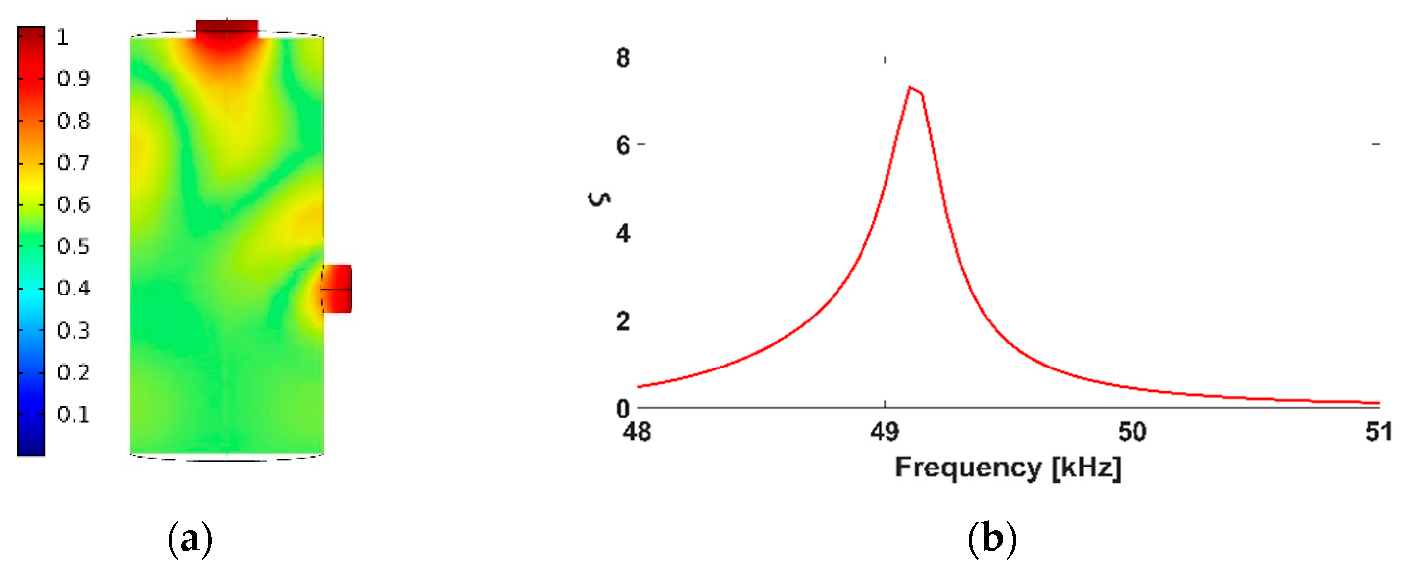
The optimization results show that the relative PA signal () of 7.23 is obtained if , and are 17.146 mm, 1.1195 mm and 6.7924 mm, respectively. The peak resonance frequency equals 49.2 kHz. Due to difficulty in resolving the superimposed resonances, we have refrained from calculating and comparing the quality factor. The pressure distribution of the optimized resonator at 49.2 kHz is shown in Figure 9. The pressure antinode is located at the position of the microphone diaphragm which is important for high detection.
3.4. Verification
The optimized resonator is manufactured for an experimental verification of the results. The production tolerance is 0.01 mm. A schematic of the resonator cross-section is shown in Figure 10.
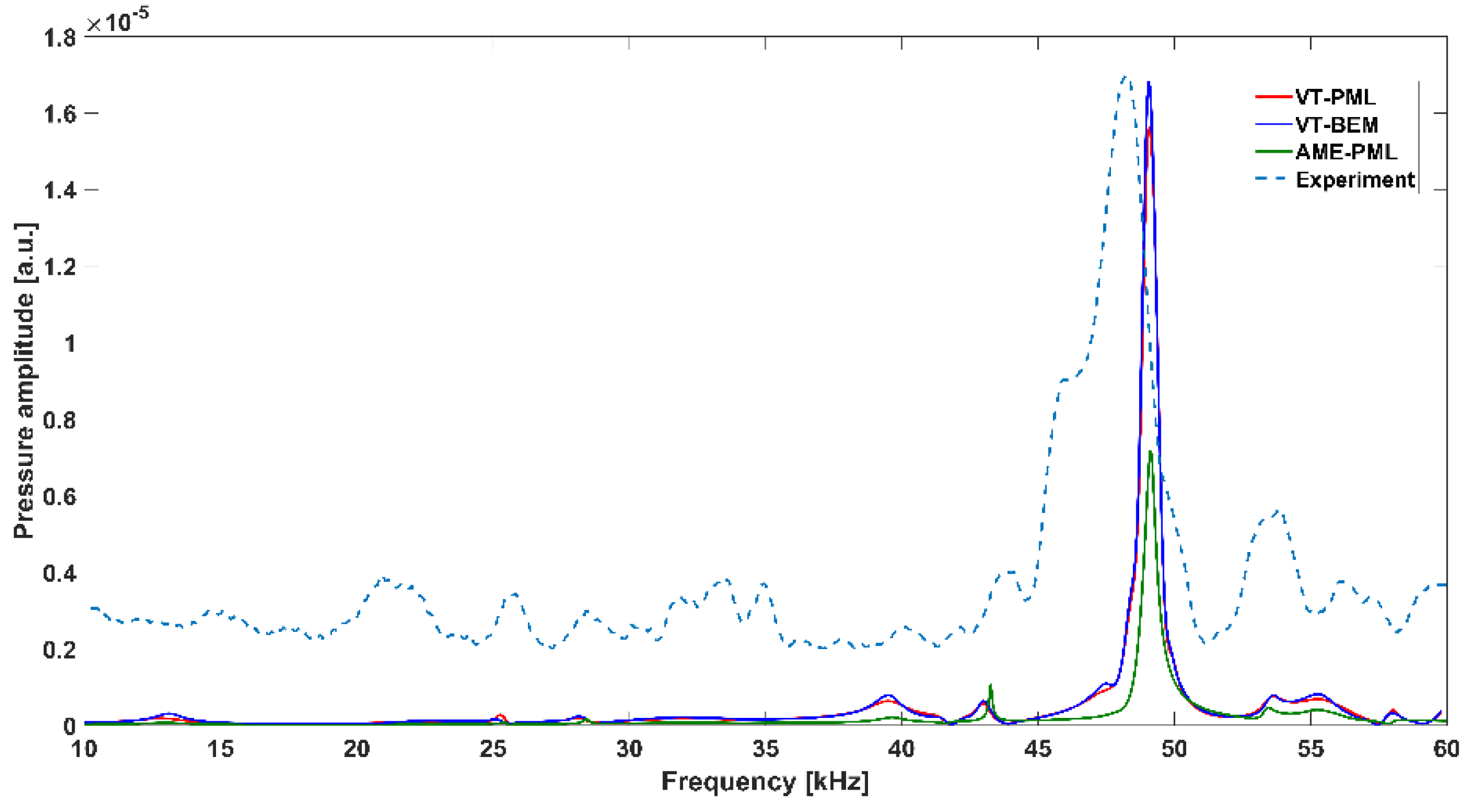
Additionally, the frequency response of the optimized resonator is calculated using the VT-PML, VT-BEM and AME-PML approaches. The AME-PML simulation is performed with frequency intervals of 10 Hz. The VT-PML and VT-BEM simulations are performed at intervals of 300 Hz and fitted with a cubic spline. The difference in the increments is because the simulation time of the AME-PML is shorter than that of the VT-PML and VT-BEM approach [21]. In order to account for the production limits, the resonator dimensions are rounded 0.01 mm. The three simulation plots are shown in Figure 11 together with the experimental results.
Experiment and simulations consistently show that the resonance with a peak at 49 kHz has by far the highest amplitude. All simulations predict similar spectral features and show a slight shift of the peak frequency from 49.2 kHz to 49.0 kHz and a decrease of from 7.23 to 4.59. This difference can be attributed to the rounded resonator dimensions, representing the production uncertainties. The new resonator represents nevertheless a significant improvement over the reference resonator.
The strongest resonance in both the measurements and the simulations spans a wide frequency range. The measured resonance frequency equals 48.3 kHz and is thus lower than the simulation results (49 kHz). This might be attributed to PA signal leakage at the microphone mount. This effect is not considered in the numerical models.
The weak resonances, recognizable in the simulations, are hard to identify in the measurement due to noise. The measured amplitude of the optimized resonator is 2.34 times larger than the amplitude of the reference resonator as seen in Figure 12.
4. Conclusions
We have described the optimization of an open T-shaped resonator designed for application in blood glucose measurements. The resonator geometry is optimized for strong PA signal in the ultrasound using finite element modelling. The method described here can be applied for the optimization of open PA resonators of arbitrary shape as well. The optimization procedure would be particularly suitable for optimizing complex resonators which have numerous design variables. The results from the optimization have been confirmed using both experimental measurements and other numerical methods. The PA signal experimentally increased by a factor of 2.34 compared to the reference resonator. This improvement constitutes an important step towards the development of a portable PA glucose sensor as we expect that it will significantly improve the sensitivity of PA glucose measurements. The next step is to validate the optimization by making in vitro PA measurements of glucose solutions before performing in vivo measurements.
Author Contributions
Conceptualization, S.E.-B., B.B., L.D. and M.W.; methodology, S.E.-B., B.B., L.D. and M.W.; software, S.E.-B.; validation, S.E.-B.; formal analysis, S.E.-B.; investigation, S.E.-B.; data curation, S.E.-B.; writing—original draft preparation, S.E.-B.; writing—review and editing, S.E.-B., B.B., L.D. and M.W.; visualization, S.E.-B.; supervision, B.B., L.D. and M.W.; project administration, S.E.-B., B.B, L.D. and M.W.; funding acquisition, B.B. and M.W. All authors have read and agreed to the published version of the manuscript.
Funding
We would like to thank the Hamburg University of Applied Science Promotionsförderung for funding.
Conflicts of Interest
The authors declare no conflict of interest.
References
- Bell, A.G. On the production and reproduction of sound by light. Am. J. Sci. 1880, 20, 305–324. [Google Scholar] [CrossRef] [Green Version]
- McClelland, J. Condensed matter photoacoustic spectroscopy and detection using gas phase signal generation. 1980 Ultrason. Symposium. 1980, 610–617. [Google Scholar] [CrossRef]
- Somoano, R.B. Photoacoustic spectroscopy of condensed matter. Angew. Chem. 1978, 17, 238–245. [Google Scholar] [CrossRef]
- Martel, R.; N’Soukpoe-Kossi, C.N.; Paquin, P.; Leblanc, R.M. Photoacoustic analysis of some milk products in ultraviolet and visible light. J. Dairy Sci. 1987, 70, 1822–1827. Available online: https://www.journalofdairyscience.org/article/S0022-0302(87)80220-5/pdf (accessed on 8 March 2021). [CrossRef]
- Döka, O.; Bicanic, D.; Szöllösy, L. Rapid and gross screening for Pb3O4 adulterant in ground sweet red paprika by means of photoacoustic spectroscopy. Instrum. Sci. Technol. 1998, 25, 203–208. [Google Scholar] [CrossRef]
- He, Y.; Shi, J.; Pleitez, M.A.; Maslov, K.I.; Wagenaar, D.A.; Wang, L.V. Label-free imaging of lipid-rich biological tissues by mid-infrared photoacoustic microscopy. J. Biomed. Opt. 2020, 25, 1–7. [Google Scholar] [CrossRef] [PubMed]
- Pleitez, M.A.; Khan, A.A.; Soldà, A.; Chmyrov, A.; Reber, J.; Gasparin, F.; Seeger, M.R.; Schätz, B.; Herzig, S.; Scheideler, M.; et al. Label-free metabolic imaging by mid-infrared optoacoustic microscopy in living cells. Nat. Biotechnol. 2020, 38, 293–296. [Google Scholar] [CrossRef] [PubMed]
- Saalberg, Y.; Bruhns, H.; Wolff, M. Photoacoustic spectroscopy for the determination of lung cancer biomarkers-a preliminary investigation. Sensors 2017, 17, 210. [Google Scholar] [CrossRef]
- Loh, A.; Wolff, M. Photoacoustic detection of short-chained hydrocarbons isotopologues. Proceedings 2019, 15, 15023. [Google Scholar] [CrossRef] [Green Version]
- Sigrist, M.W. Trace gas monitoring by laser-photoacoustic spectroscopy. Infrared Phys. Technol. 1995, 36, 415–425. [Google Scholar] [CrossRef]
- Tomberg, T.; Vainio, M.; Hieta, T.; Halonen, L. Sub-parts-per-trillion level sensitivity in trace gas detection by cantilever-enhanced photoacoustic spectroscopy. Sci. Rep. 2018, 8, 1848. [Google Scholar] [CrossRef] [Green Version]
- Dumitraş, D.C.; Dutu, D.C.; Matei, C.; Magureanu, A.M.; Petrus, M.; Popa, C. Laser photoacoustic spectroscopy: Principles, instrumentation, and characterization. J. Optoelectron. Adv. Mater. 2007, 9, 3655–3701. [Google Scholar]
- Pleitez, M.A.; Lieblein, T.; Bauer, A.; Hertzberg, O.; Lilienfeld-Toal, H.V.; Mäntele, W. Windowless ultrasound photoacoustic cell for in vivo mid-IR spectroscopy of human epidermis: Low interference by changes of air pressure, temperature, and humidity caused by skin contact opens the possibility for a non-invasive monitoring of glucose in the interstitial fluid. Rev. Sci. Instrum. 2013, 84, 084901. [Google Scholar] [CrossRef]
- Sim, J.Y.; Ahn, C.-G.; Jeong, E.-J.; Kim, B.K. In vivo microscopic photoacoustic spectroscopy for non-invasive glucose monitoring invulnerable to skin secretion products. Sci. Rep. 2018, 8, 1059. [Google Scholar] [CrossRef] [PubMed] [Green Version]
- Bijnen, F.G.C.; Reuss, J.; Harren, F.J.M. Geometrical optimization of a longitudinal resonant photoacoustic cell for sensitive and fast trace gas detection. Rev. Sci. Instrum. 1996, 67, 2914–2923. [Google Scholar] [CrossRef] [Green Version]
- Kost, B.; Baumann, B.; Germer, M.; Wolff, M.; Rosenkranz, M. Numerical shape optimization of photoacoustic resonators. Appl. Phys. B 2011, 102, 87–93. [Google Scholar] [CrossRef]
- Wolff, M.; Kost, B.; Baumann, B. Shape-Optimized Photoacoustic Cell: Numerical Consolidation and Experimental Confirmation. Int. J. Thermophys. 2012, 33, 1953–1959. [Google Scholar] [CrossRef]
- Cotterell, M.I.; Ward, G.P.; Hibbins, A.P.; Haywood, J.M.; Wilson, A.; Langridge, J.M. Optimizing the performance of aerosol photoacoustic cells using a finite element model. Part 1: Method validation and application to single-resonator multipass cells. Aerosol. Sci. Technol. 2019, 53, 1107–1127. [Google Scholar] [CrossRef] [Green Version]
- Cotterell, M.I.; Ward, G.P.; Hibbins, A.P.; Haywood, J.M.; Wilson, A.; Langridge, J.M. Optimizing the performance of aerosol photoacoustic cells using a finite element model. Part 2: Application to a two-resonator cell. Aerosol. Sci. Technol. 2019, 53, 1128–1148. [Google Scholar] [CrossRef] [Green Version]
- Sim, J.Y.; Ahn, C.-G.; Huh, C.; Chung, K.H.; Jeong, E.-J.; Kim, B.K. Synergetic resonance matching of a microphone and a photoacoustic cell. Sensors 2017, 17, 804. [Google Scholar] [CrossRef] [PubMed] [Green Version]
- El-Busaidy, S.A.S.; Baumann, B.; Wolff, M.; Duggen, L. Modelling of open photoacoustic resonators. Photoacoustics 2020, 18, 100161. [Google Scholar] [CrossRef] [PubMed]
- El-Busaidy, S.A.S.; Baumann, B.; Wolff, M.; Duggen, L.; Bruhns, H. Experimental and numerical investigation of a photoacoustic resonator for solid samples: Towards a Non-Invasive Glucose Sensor. Sensors 2019, 19, 2889. [Google Scholar] [CrossRef] [PubMed] [Green Version]
- Comsol Multiphysics Optimization Module User’s Guide Version 5.4; COMSOL Multiphysics: Stockholm, Sweden, 2018.
- MATLAB-Homepage. Available online: https://www.mathworks.com (accessed on 14 January 2021).
- Miklós, A.; Hess, P.; Bozóki, Z. Application of acoustic resonators in photoacoustic trace gas analysis and metrology. Rev. Sci. Instrum. 2001, 72, 1937–1955. [Google Scholar] [CrossRef] [Green Version]
Figure 1.
Schematic of the experimental setup.

Figure 2.
(a): Cross-sectional view of the T-shaped reference resonator (white). The dashed lines represent the cylindrical symmetry axes. (b): 3D view of the resonator. The resonator is rotated compared to the resonator depicted in the schematic of the experimental setup (Figure 1).
Figure 2.
(a): Cross-sectional view of the T-shaped reference resonator (white). The dashed lines represent the cylindrical symmetry axes. (b): 3D view of the resonator. The resonator is rotated compared to the resonator depicted in the schematic of the experimental setup (Figure 1).

Figure 3.
Frequency response of the reference resonator from the viscothermal model with perfectly matched layers (VT-PML) simulation and measurement. The measurement and simulation results are scaled for easier viewing and comparison.
Figure 3.
Frequency response of the reference resonator from the viscothermal model with perfectly matched layers (VT-PML) simulation and measurement. The measurement and simulation results are scaled for easier viewing and comparison.

Figure 4.
Relative photoacoustic (PA) signal of the coarse resonance cylinder sweep (a) along with a contour plot (b). The color scale gives the values of . The peak highlighted in the left plot is the region with the highest relative PA signal.
Figure 4.
Relative photoacoustic (PA) signal of the coarse resonance cylinder sweep (a) along with a contour plot (b). The color scale gives the values of . The peak highlighted in the left plot is the region with the highest relative PA signal.

Figure 5.
The absolute pressure distribution plots of the six peaks. The plots are normalized by the highest value of the individual plot. Top: resonance cylinder position () 4 mm (a) and 5 mm (b,c). Bottom: resonance cylinder position ( ) 12 mm. The length of the resonance cylinder ( ) is 1 mm, 8 mm and 15 mm respectively.

Figure 6.
Relative PA signal of the finer resonance cylinder sweep (a) along with a contour plot (b). The color scale gives the values of .
Figure 6.
Relative PA signal of the finer resonance cylinder sweep (a) along with a contour plot (b). The color scale gives the values of .

Figure 7.
Relative PA signal of the coarse cavity cylinder sweep (a) along with a contour plot (b). The color scale gives the values of . The peak highlighted in the left plot is the region with the highest relative PA signal.
Figure 7.
Relative PA signal of the coarse cavity cylinder sweep (a) along with a contour plot (b). The color scale gives the values of . The peak highlighted in the left plot is the region with the highest relative PA signal.

Figure 8.
Relative PA signal of the combined sweep of and (a) along with a contour plot (b). The color scale gives the values of .
Figure 8.
Relative PA signal of the combined sweep of and (a) along with a contour plot (b). The color scale gives the values of .

Figure 9.
(a): Absolute pressure distribution inside the optimized resonator at 49.2 kHz. (b): Relative PA signal of the optimized resonator around 49.2 kHz.
Figure 9.
(a): Absolute pressure distribution inside the optimized resonator at 49.2 kHz. (b): Relative PA signal of the optimized resonator around 49.2 kHz.

Figure 10.
Schematic of the cross-section of the optimized resonator, dimensions in mm. The dashed lines represent the cylindrical symmetry axes.
Figure 10.
Schematic of the cross-section of the optimized resonator, dimensions in mm. The dashed lines represent the cylindrical symmetry axes.

Figure 11.
Frequency response of the experiment against the simulations of the optimized resonator. The blue, red and green plots represent the VT-PML, VT-BEM and AME-PML approach, respectively. The blue dashed line shows the experimental measurement.
Figure 11.
Frequency response of the experiment against the simulations of the optimized resonator. The blue, red and green plots represent the VT-PML, VT-BEM and AME-PML approach, respectively. The blue dashed line shows the experimental measurement.

Figure 12.
Frequency response plot of the reference resonator with the optimized resonator.


Table 1.
Resonator dimensions.
| Dimensions in mm | |
|---|---|
| Absorption cylinder length | 0.7681 |
| Absorption cylinder radius | 1.2706 |
| Cavity cylinder length | 15.2713 |
| Cavity cylinder radius | 4.0074 |
| Resonance cylinder length | 8.1146 |
| Resonance cylinder radius | 1.0105 |
| Resonance cylinder position | 6.1067 |
Table 2.
Range of optimization variables.
| Optimization Variables | Range (mm) |
|---|---|
| Resonance cylinder length | 1–8 |
| Resonance cylinder position | 6–8 |
| Cavity cylinder length | 16.9–17.2 |
Publisher’s Note: MDPI stays neutral with regard to jurisdictional claims in published maps and institutional affiliations. |
© 2021 by the authors. Licensee MDPI, Basel, Switzerland. This article is an open access article distributed under the terms and conditions of the Creative Commons Attribution (CC BY) license (http://creativecommons.org/licenses/by/4.0/).
Share and Cite
MDPI and ACS Style
El-Busaidy, S.; Baumann, B.; Wolff, M.; Duggen, L. Shape Optimization of an Open Photoacoustic Resonator. Appl. Sci. 2021, 11, 2571. https://0-doi-org.brum.beds.ac.uk/10.3390/app11062571
AMA Style
El-Busaidy S, Baumann B, Wolff M, Duggen L. Shape Optimization of an Open Photoacoustic Resonator. Applied Sciences. 2021; 11(6):2571. https://0-doi-org.brum.beds.ac.uk/10.3390/app11062571
Chicago/Turabian StyleEl-Busaidy, Said, Bernd Baumann, Marcus Wolff, and Lars Duggen. 2021. "Shape Optimization of an Open Photoacoustic Resonator" Applied Sciences 11, no. 6: 2571. https://0-doi-org.brum.beds.ac.uk/10.3390/app11062571
Note that from the first issue of 2016, this journal uses article numbers instead of page numbers. See further details here.