Strain Sensitivity Enhancement of Broadband Ultrasonic Signals in Plates Using Spectral Phase Filtering

Abstract

The focused signal obtained by the time-reversal or the cross-correlation techniques of ultrasonic guided waves in plates changes when the medium is subject to strain, which can be used to monitor the medium strain level. In this paper, the sensitivity to strain of cross-correlated signals is enhanced by a post-processing filtering procedure aiming to preserve only strain-sensitive spectrum components. Two different strategies were adopted, based on the phase of either the Fourier transform or the short-time Fourier transform. Both use prior knowledge of the system impulse response at some strain level. The technique was evaluated in an aluminum plate, effectively providing up to twice higher sensitivity to strain. The sensitivity increase depends on a phase threshold parameter used in the filtering process. Its performance was assessed based on the sensitivity gain, the loss of energy concentration capability, and the value of the foreknown strain. Signals synthesized with the time–frequency representation, through the short-time Fourier transform, provided a better tradeoff between sensitivity gain and loss of energy concentration.

1. Introduction

Mechanical strain measurement and monitoring are vital in several areas of engineering [1,2,3]. Ultrasonic waves can be used for monitoring strain by measuring the time-shift of received signals [4] since the propagation speed of an ultrasonic wave is proportional to the stress level of the medium, according to the acoustoelastic theory [5,6]. Ultrasonic guided waves are generally dispersive and multimodal but are widely used in the non-destructive evaluation and structural health monitoring since they can propagate long distances and inspect a large area [7]. The influence of strain on ultrasonic guided waves is, however, more complex than on bulk waves: each guided wave mode presents different sensitivity to strain, which also depends on the frequency [8,9,10,11,12,13]. That is, at each frequency, the time-shift that each mode may experience is different. Experimental strain measurement with ultrasonic guided waves is usually performed by observing the time-shift of a single guided wave mode [8,14,15,16]. This, however, requires very accurate time-shift measuring and single-mode excitation, which may not be straightforwardly achievable in different types of structure.

A wideband excitation in a plate can, in principle, generate several guided wave modes and thus identification of individual time-shifts can be complicated. If the medium presents features that allow scattering [17] and mode conversion [18,19] the received signals can be even more complex. The time-reversal technique can be used to compensate this complex behavior creating a focused signal. If the received signal, which may be composed of several modes and scattered waves, is reversed in time and retransmitted, then propagation related phenomena, such as scattering and dispersion, are compensated producing a sharp peak in the next received signal [20]. Several researchers used the time-reversal technique on guided waves in order to identify the presence of defects in plates [21,22,23,24,25,26].

In previous work, the time-reversal signal processing, either physically or numerically implemented via cross-correlation, was applied to evaluate the variation of the longitudinal tensile stress in plates [27]. The main principle of the technique lies in exploiting the complex propagating behavior, in which several wave modes distributed over a wide frequency range are excited. These several components potentially present different sensitivity to strain, therefore mismatching the system transfer function due to the presence of stress, which reduces the focusing capability of the process and, in turn, decreases the peak of the final signal, being therefore easily observable. A similar procedure was applied to concrete pillars [28] showing that different time-intervals of the received signal present different sensitivity to strain. Quiroga et al. [29] excited several guided wave modes in a rod and pipe subjected to axial and bending stress, respectively. It has been observed that, due to the different speed variation for the several modes presented in the received signal, stress evaluation through speed measurements was indeed a complex task. They adopted a principal component analysis in order to monitor stress.

When several wideband modes propagate, the received signal may be quite complex to analyze since the individual signals from each mode may be distributed over time and with different frequency content. Thus, identification of individual wave packets in either time or frequency domains is usually not possible. However, they can be better distinguished through time–frequency representations [30,31,32,33] such as the short-time Fourier transform (STFT). Time–frequency analysis was applied to ultrasonic guided waves before, to increase the detectability of defects in plates [34,35] and pipes [36,37].

In this paper, we modify the original cross-correlation strain monitoring procedure [27] aiming to investigate whether the sensitivity to strain could be increased. It is modified by using a new signal as reference which is synthesized relying on the system impulse response at some foreknown strain level. The new reference signal is obtained by means of a post-processing filter based on the phase of either the Fourier transform or the short-time Fourier transform. The latter allows one to analyze how several signal components are affected by strain in both the time and frequency domains, being therefore suitable to cases where several wave modes arrive distributed over time and at different frequencies, such as wideband guided waves. The idea of using synthesized signals for strain monitoring through the phase of the Fourier transform was briefly proposed by Martinho et al. [38]. Here, it is comprehensively extended by comparing it to the short-time Fourier transform and assessing the effectiveness of the technique with regards to the foreknown strain level and on the loss of energy concentration capability.

The rest of the paper is organized as follows. Section 2 explains the strain effect on ultrasonic guided waves and the original procedure for strain monitoring. Section 3 devises the modified procedure using the information of the phase of the Fourier and short-time Fourier transforms. Section 4 presents the results with experimental signals and Section 5 draws the conclusions.

2. Theoretical Background

2.1. Strain Effect on Guided Waves

According to the acoustoelastic effect, the propagation speed of ultrasonic waves changes as a function of the medium stress state [5]. The speed variation for bulk waves depends not only on the stress intensity but on its direction and is different for longitudinal and shear wave modes. In addition, there may be a geometric change in the medium, due to stress, which alters the propagation path. Thus, due to the change of the wave speed and propagation path, the propagation time of an ultrasonic wave changes with strain. This principle allows for measuring the strain level.

Plates support the propagation of guided waves. In an isotropic plate, there are two families of guided waves, namely Lamb and SH waves [39]. For each of them, there exist, in principle, infinite propagating modes: the number of propagating modes increases with the frequency. These guided waves modes are generally dispersive which means that their phase and group speeds change with frequency. The dependence on strain for guided waves is more complex than for bulk waves [8,9,10,13]. Each guided wave mode presents different speed variation which also depends on the frequency. For instance, the A0 Lamb wave mode presents either positive or negative speed variation depending on the frequency for uniaxial stress applied along the propagation direction [8]. It has also been observed that close to a mode’s cut-off frequency the speed variation can be very intense [9].

When a broadband pulse is applied to an ultrasonic transducer in a plate, potentially several dispersive guided wave modes may be generated. Due to this dispersive and multimodal behavior, it may be complicated to interpret the received signal, which may be composed by the interference of these several waves. The signal is yet more complex when there are scattering from features in the plate, such as reflections from the plate’s end. In this scenario, if the plate is subjected to stress, each mode presents a different time-shift, and, due to the aforementioned nature of the received signal, quantitative identification of the stress effect in such a complex signal is impractical without resorting to some signal analysis technique [27,28,29]. In the next subsection, a strain monitoring approach that exploits the aforementioned complex behavior is summarized.

2.2. Strain Monitoring through Cross-Correlation or Time-Reversal Signals

In a plate-like structure, the time-reversal technique is a process that compensates for the multimodal and dispersive behavior, allowing all the propagating modes to arrive synchronously at the reception point, producing a focused and recompressed signal [20]. This process is numerically equivalent to the cross-correlation of the system impulse response, as shown previously [27]. In this paper, the numerical approach is used. It can be summarized as follows.

Consider a plate with two ultrasonic transducers positioned on its surface; one is used as a transmitter and the other as a receiver, where transmitter and receiver are separated by a predefined distance. First, an impulse-like signal is sent from the transmitter. This produces a response signal in the receiver, say $h\left(t\right)$. This signal can be considered as the impulse response of the system that includes both transmitter and receiver acoustoelectric responses and all wave propagation related phenomena, such as dispersion, multimodal behavior, scattering and mode conversion. The signal $h\left(t\right)$ obtained in this step is the reference signal for the remaining steps. In the next step, $h\left(t\right)$ is convolved with its time-reversed version, $h(-t)$, yielding

$$y\left(t\right)=h(-t)\ast h\left(t\right),$$

(1)

where the symbol ∗ means convolution. Note that the signal $y\left(t\right)$ is the cross-correlation of the system impulse response, $h\left(t\right)$, with itself.

The signal $y\left(t\right)$ is numerically equivalent to the time-reversal focused signal, obtained by exciting the transmitter with $h(-t)$, in which the dispersion and multimodal behavior are compensated [20,27], making $y\left(t\right)$ to be maximum at its focusing instant where it presents a high amplitude main peak. To quantify the focusing capability, time-reversal energy efficiency (TREF), introduced in [27], can be used. It is defined as the ratio of the energy in the central peak to the energy of the whole signal, as stated by Equation (2):

$$\mathrm{TREF}\left\{y\left(t\right)\right\}=\frac{{\int }_{t_1}^{t_2}{y}^2\left(t\right)dt}{{\int }_{-\infty }^{\infty }{y}^2\left(t\right)dt}.$$

(2)

The central peak is defined as the signal between the first zero-crossing immediately before and after the main positive peak, $t_1$ and $t_2$ in Equation (2). The higher is the TREF, the more concentrated is the signal’s energy in the central peak.

When strain is imposed on the plate and the same reference signal remains, the focusing capability decreases with the strain level. This fact can be used as a way to monitor strain changes in the medium [27]. This can be understood by assuming that the transfer functions in the first and second steps are no longer the same due to the change in each mode’s speed, according to the acoustoelastic theory [8,9,10], and propagating path. Considering that the first step is performed under no strain and the second step is performed under longitudinal strain, Equation (1) becomes the cross-correlation of both impulse responses:

$$y(\epsilon ,t)=h(0,-t)\ast h(\epsilon ,t),$$

(3)

where $h(0,t)$ is the reference signal under zero-strain and $h(\epsilon ,t)$ is the impulse response of the system when the plate is subjected to strain $\epsilon$. This process is summarized in Figure 1. Comparing Equations (1) and (3), one can conclude that strain changes the system from $h(0,t)$ to $h(\epsilon ,t)$, thus introducing a mismatch to the system response signal and consequently decreasing the main peak of $y(\epsilon ,t)$, compared to $y\left(t\right)$. Thus, the complex propagating behavior of the medium allows strain variation to be easily monitored by observing the changes on the main peak. The peak reduction is however subtle. In the next section, a procedure that provides a new reference signal, to be used instead of $h(0,t)$, that increases the sensitivity to strain on $y(\epsilon ,t)$ is presented.

2.3. Fourier and Short-Time Fourier Transforms

The filtering techniques developed in this paper use two transforms in order to analyze the signals’ frequency content, namely the Fourier transform (FT) and the short time Fourier transform (STFT) [40]. They are defined, respectively, as follow:

$$\mathcal{F}\left\{y\left(t\right)\right\}=Y\left(f\right)={\int }_{-\infty }^{\infty }y\left(t\right)e^{-j2\pi ft}dt,$$

(4)

$$\mathcal{SF}\left\{y\left(t\right)\right\}=Y(\tau ,f)={\int }_{-\infty }^{\infty }y\left(t\right)w(t-\tau )e^{-j2\pi ft}dt,$$

(5)

where $w\left(t\right)$ is a window function. Here, a Blackman window function is used, which is defined by:

$$w\left(t\right)=\left\{\begin{array}{cc}0.42+0.5cos\left(\frac{2\pi t}{T}\right)+0.08cos\left(\frac{4\pi t}{T}\right),\hfill & -\frac{T}{2}\le t\le \frac{T}{2}\hfill \\ 0,\hfill & \mathrm{otherwise}\hfill \end{array}\right.,$$

(6)

with T being the length of the window. For the signals treated here, as presented in Section 4, the temporal length of the window, T, and the overlap length of consecutive windows were set to $50 \mu s$ and $93\%$ of the window length, respectively, since these values showed good compromise between time and frequency resolution.

These transforms provide information on the frequency content of the acquired signal. In the latter, the frequency content is analyzed as a function of time, $\tau$, since only the content inside the time window, $w(t-\tau )$, centered at the time instant $\tau$, is considered. The signal in the time domain can be recovered by the inverse Fourier and short-time Fourier transforms [40].

3. Filtering Procedure for Synthesis of a New Reference Signal

In this work, the aforementioned strain monitoring process is modified to increase the strain sensitivity of the signal $y(\epsilon ,t)$ in Equation (3). This is accomplished by using a modified reference signal which is synthesized through a phase filter that relies on the prior knowledge of the system response at some non-zero strain state. The filtering technique is performed as follows.

First, the impulse response signal under null strain, $h(0,t)$, and under some non-zero strain, $\tilde{\epsilon }$, $h(\tilde{\epsilon },t)$, are acquired and addressed in the frequency domain, through one of the transforms described in Section 2.3, here generically represented as $\mathcal{T}\{·\}$:

$$H(0,\chi )=\mathcal{T}\left\{h\right(0,t\left)\right\}$$

(7)

and

$$H(\tilde{\epsilon },\chi )=\mathcal{T}\left\{h(\tilde{\epsilon },t)\right\},$$

(8)

respectively, where $\chi$ is the transform variable, i.e., either $\chi =f$ for FT or $\chi =(\tau ,f)$ for STFT. Then, these two signals are cross-correlated, which is performed by multiplying them in the transform domain:

$$S_{\tilde{\epsilon }}\left(\chi \right)=H^{\ast }(0,\chi )H(\tilde{\epsilon },\chi ),$$

(9)

where the asterisk superscript means complex conjugate. Note that the phase of $S_{\tilde{\epsilon }}\left(\chi \right)$ represents the phase shift between the two impulse responses, $h(0,t)$ and $h(\tilde{\epsilon },t)$, as a function of $\chi$. Considering that the strain-induced speed and path changes mainly affect the phase of the received wave packets, and assuming that the major difference between $h(0,t)$ and $h(\tilde{\epsilon },t)$ is caused by strain, it is interesting to analyze the phase of $S_{\tilde{\epsilon }}\left(\chi \right)$, which presents high absolute values for the spectral components that are more affected by strain, i.e., the more sensitive components. Based on this principle, one can define the $\varphi$-sensitive coefficients as the ones whose phase of $S_{\tilde{\epsilon }}\left(\chi \right)$ is greater than $\varphi$. Therefore, a zero-one function, $M_{\varphi ,\tilde{\epsilon }}\left(\chi \right)$, is built, accordingly:

$$M_{\varphi ,\tilde{\epsilon }}\left(\chi \right)=\left\{\begin{array}{cc}1,\hfill & \left|\angle S_{\tilde{\epsilon }}\left(\chi \right)\right|\ge \varphi \hfill \\ 0,\hfill & \left|\angle S_{\tilde{\epsilon }}\left(\chi \right)\right|<\varphi \hfill \end{array}\right..$$

(10)

The actual filtering step consists of multiplying $M_{\varphi ,\tilde{\epsilon }}\left(\chi \right)$ by the spectrum of the original reference signal under null strain:

$$H_{\varphi ,\tilde{\epsilon }}\left(\chi \right)=M_{\varphi ,\tilde{\epsilon }}\left(\chi \right)H(0,\chi ).$$

(11)

This process creates a new signal, $H_{\varphi ,\tilde{\epsilon }}\left(\chi \right)$, in which the coefficients that were deemed unfit, i.e., with low sensitivity, are eliminated. Lastly, $H_{\varphi ,\tilde{\epsilon }}\left(\chi \right)$ is transformed back to the time-domain, by the inverse of the chosen transform:

$$h_{\varphi ,\tilde{\epsilon }}\left(t\right)={\mathcal{T}}^{-1}\left\{H_{\varphi ,\tilde{\epsilon }}\left(\chi \right)\right\}.$$

(12)

The filtering process is summarized in Figure 2. This new time-domain signal is used as reference for the original monitoring procedure, as explained in Section 2.1. More precisely, $h_{\varphi ,\tilde{\epsilon }}\left(t\right)$ should be used instead of $h(0,t)$ in Equation (3), which becomes:

$$y_{\varphi }(\epsilon ,t)=h_{\varphi ,\tilde{\epsilon }}(-t)\ast h(\epsilon ,t).$$

(13)

It is worth highlighting that the present method considers that the main cause of phase-shifting is strain. However, temperature variation can also induce phase variations since it changes the wave speed and propagation path [41,42]. In this paper, temperature is assumed constant. Alternatively, the present method can, in principle, be applied in scenarios where one intends to select the most temperature-sensitive components when strain remains constant.

Observing Equation (10), one can see that, when $\varphi =0^{\circ }$, the original signal remains unaltered, i.e., it is not filtered and Equation (13) is equivalent to Equation (3), whereas, when $\varphi ={180}^{\circ }$, all of the original signal is filtered out, thus $H_{\varphi ,\tilde{\epsilon }}\left(\chi \right)$ is nullified. That is, the higher is the value of $\varphi$ in $M_{\varphi ,\tilde{\epsilon }}\left(\chi \right)$ in Equation (10), the more sensitive to strain is the focused signal, $y_{\varphi }(\epsilon ,t)$ in Equation (13). The choice for an adequate value of $\varphi$ depends on the system under study. Another parameter that affects the sensitivity of the technique is the choice of the foreknown strain value, $\tilde{\epsilon }$. If $\tilde{\epsilon }$ is low, then the effect of strain on the ultrasonic wave is less intense and the signal $h(\epsilon ,t)$ is not too different from $h(0,t)$. Thus, if one takes two values of $\tilde{\epsilon }$, namely low and high values, for the same threshold angle, $\varphi$, the former would, ideally, provide a filtered signal, $h_{\varphi ,\tilde{\epsilon }}\left(t\right)$, that is more sensitive to strain, since the selected components present a phase shift of at least $\varphi$ with low strain. In the next section, results obtained with FT and STFT techniques for several threshold angles and different foreknown strain are shown.

4. Results and Discussion

Experiments were performed with a pair of piezocomposite transducers in a 3-mm-thick, 800-mm-long and 100-mm-wide aluminum plate where transmitter and receiver were placed close to each end of the plate, separated by 700 mm. The plate is mounted over a bridge structure where variable tensile stress along the plate’s length can be applied, as schematically shown in Figure 3, following the setup used in [27]. Piezocomposite transducers were used due to their wider bandwidth, compared to conventional piezoelectric ceramics. They were prepared following the standard dice and fill procedure [43] with a 0.65 mm thick PZ37 ceramic from Ferroperm [44] and widths of element and polymer of 0.1 and 0.04 mm, respectively, and 0.14 mm pitch. One ultrasonic transducer was used as transmitter and the opposite as receiver.

An initial broadband pulse excites the transmitter generating several wave modes in the plate which propagate until being received by the opposite transducer. Here, reflections from the plate’s ends were received, due to the transducer positioning, which, to some extent, increase the number of wave packets that arrive at the receiver. Figure 4 shows the reference signal, $h(0,t)$, acquired due to the first propagating step, its Fourier and short-time Fourier transforms. The complex wave propagating phenomenon can be verified in Figure 4a, as multiple wave packets arrive at different time instants, with different frequency components. The cross-correlated focused signal under null strain, $y\left(t\right)$, obtained through Equation (3), is shown in Figure 5. As can be seen, it has a high main peak, which concentrates a significant amount of the signal’s energy.

4.1. Fourier Transform Filter Implementation

The filtering technique is applied to the reference signal using initially the Fourier transform. That is, the transform $\mathcal{T}$ is the Fourier transform and the transform variable $\chi$ is the frequency. The function $M_{\varphi ,\tilde{\epsilon }}\left(f\right)$ is calculated with a reference strain value, $\tilde{\epsilon }$, of about 150 $\mu \epsilon$ (where the unit $\mu \epsilon$ is a short notation for a strain of $\mu m/m$) as per Equation (10), and then used to compute the new reference, $H_{\varphi ,\tilde{\epsilon }}\left(f\right)$, according to Equation (11) and Figure 2. To illustrate the influence of the angle threshold, $\varphi$, Figure 6 shows the $M_{\varphi ,\tilde{\epsilon }}\left(f\right)$ function calculated with two values of $\varphi$, namely $\varphi ={15}^{\circ }$ and $\varphi ={30}^{\circ }$. One can see that they assume values zero or one, and, comparing their shapes, the $M_{\varphi ,\tilde{\epsilon }}\left(f\right)$ function with $\varphi ={30}^{\circ }$ (Figure 6b) is sparser around the unit because more frequency components are nullified than the one obtained with $\varphi ={15}^{\circ }$ (Figure 6a). This holds because there are fewer components that are $\varphi$-sensitive to strain with a higher and more restrictive threshold. Figure 7 shows the respective reference signals obtained with these two $M_{\varphi ,\tilde{\epsilon }}\left(f\right)$ functions where amplitude is normalized with respect to the original signal, $h(0,t)$. One can see that, with a higher value of $\varphi$, more frequency components are filtered out by $M_{\varphi ,\tilde{\epsilon }}\left(f\right)$ according to Figure 6. Consequently, the time-domain signal of the latter is less similar to the original reference signal $h(0,t)$, shown in Figure 4a and Figure 7b, for the sake of comparison.

The focused signals after filtering, $y_{\varphi }(0,t)$, with $\varphi ={15}^{\circ }$ and $\varphi ={30}^{\circ }$, are shown in Figure 8b,c, respectively. Their amplitudes were normalized with respect to $y(0,t)$ (Figure 8a). One can see that their shapes were changed due to the filtering procedure when compared to the original focused signal, $y(0,t)$. Furthermore, the focused signal obtained with $\varphi ={30}^{\circ }$ is clearly more altered than the one obtained with $\varphi ={15}^{\circ }$, due to the removal of more frequency components, as shown in Figure 7; those frequency components were the ones recognized by $M_{\varphi ,\tilde{\epsilon }}\left(f\right)$ as low-sensitive with the corresponding threshold $\varphi$. One can also notice that the signal level away from the focus instant is more intense with $\varphi ={30}^{\circ }$ than with $\varphi ={15}^{\circ }$. That is, the former has a lower TREF.

Figure 9 shows the behavior of peak amplitude decrease, in percent, as a function of strain for the original and filtered procedure for one realization of a loading experiment. In the former, the reference signal is $h(0,t)$ (blue dots), whereas, in the latter, it is $h_{\varphi ,\tilde{\epsilon }}\left(t\right)$ with $\varphi ={30}^{\circ }$ (red dots). As can be seen, the filtering procedure made the focus peak amplitude to decrease more as strain is imposed in the plate. To quantify the sensitivity, the angular coefficient of a linear fit of the experimental peak decrease was calculated and is shown as the continuous lines in Figure 9. These values are reported in

Table 1. Sensitivity and TREF for FT and STFT filtering.

$\mathit{\varphi }$ (deg.)	FT—Filtering			STFT—Filtering
	TREF (%)	Peak Sensitivity		TREF (%)	Peak Sensitivity
		Mean (%/$\mathit{\mu }\mathit{\epsilon }$)	Std. (%/$\mathit{\mu }\mathit{\epsilon }$)		Mean (%/$\mathit{\mu }\mathit{\epsilon }$)	Std. (%/$\mathit{\mu }\mathit{\epsilon }$)
$0^{\circ }$	11.96	0.1261	0.0009	11.96	0.1261	0.0009
${15}^{\circ }$	7.67	0.1345	0.0011	8.46	0.1369	0.0010
${30}^{\circ }$	4.69	0.1635	0.0016	6.28	0.2363	0.0020
${60}^{\circ }$	2.11	0.5064	0.0044	2.26	0.5074	0.0048

, where the first row, referred to $\varphi =0^{\circ }$, presents the results obtained without any filtering. The sensitivity is reported through the mean and standard deviation (std.) of the angular coefficient. These values were calculated considering four loading experiment, where each one contains at least five acquisitions for each evaluated strain value. The TREF values, in percent, for the focused signal at null strain, shown in Figure 8, are also reported in Table 1. As can be seen, the increase of sensitivity comes at a price, as the energy focusing efficiency decreased, i.e., lower TREF was obtained. It is worth noting that the TREF values in Table 1 were computed considering the whole acquisition window shown in Figure 5 and Figure 8 to calculate the energy in the denominator of Equation (2). This time window encompasses almost all the non-negligible amplitude. If a narrower acquisition window around the peak were used, higher values would be found, but the same overall behavior with the increase of $\varphi$ would be obtained.

The amplitude sensitivity and the TREF behavior as a function of the threshold angle $\varphi$ are shown in Figure 10 by the continuous lines. One can see that, as $\varphi$ increases, sensitivity increases, until about ${70}^{\circ }$ where it reaches about $0.6\%/\mu \epsilon$, approximately fivefold the original value. However, TREF tends to decrease almost monotonically. At about ${70}^{\circ }$, TREF is just $1.25\%$, an extremely low value, meaning that the reference signal is so altered that it no longer correlates with the system’s impulse response. Signals with very poor energy concentration compromise monitoring through peak observation since it may not produce a clearly identifiable main peak.

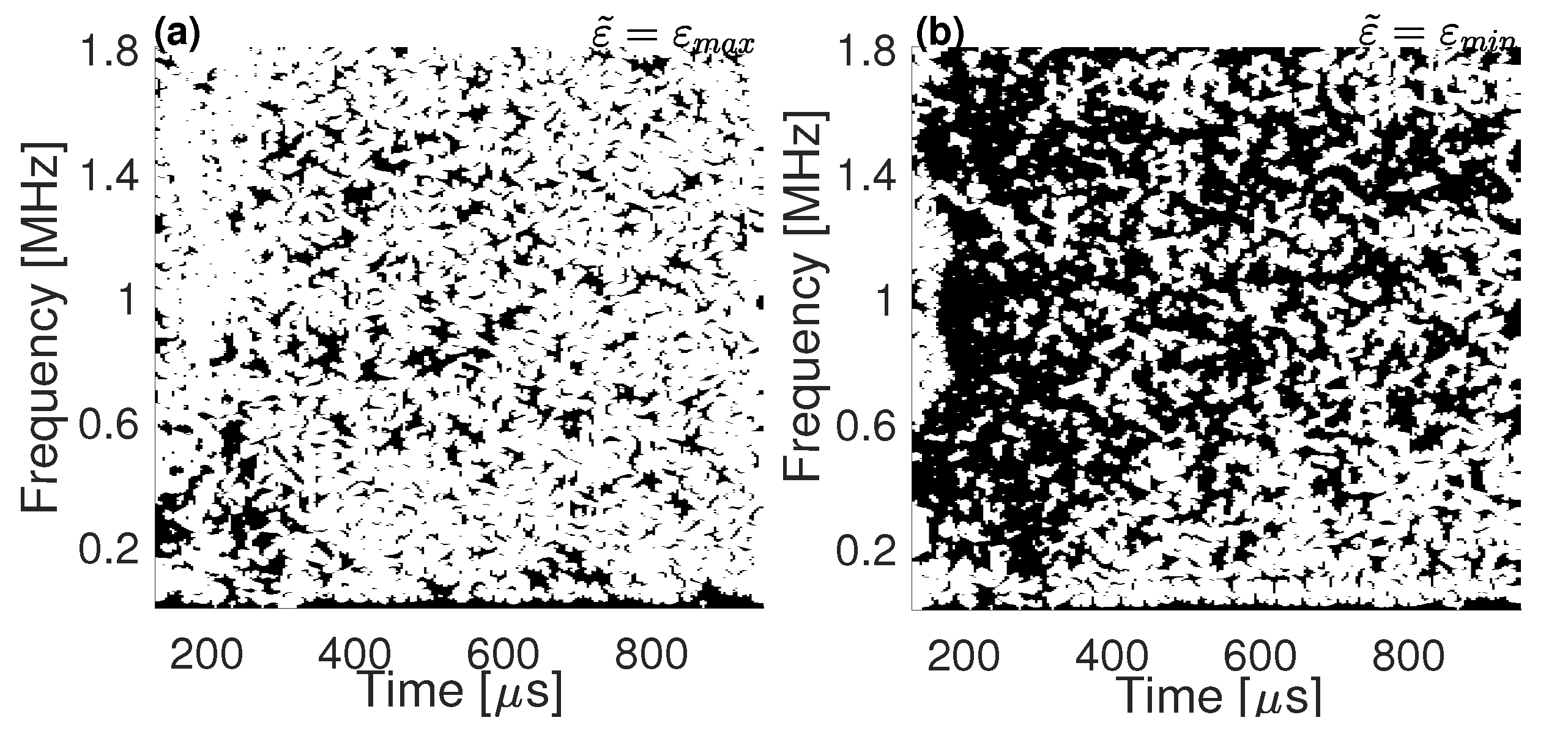
4.2. Short-Time Fourier Transform Implementation

The filtering technique with the short-time Fourier transform is evaluated. Now, the transform, $\mathcal{T}$, is STFT and, consequently, the transform variable, $\chi$, is the pair frequency and window time instant. The received signal is composed of several dispersive waves distributed over time and in the frequency spectrum, as shown in Figure 4c. Since each wave packet may have different sensitivity to strain, a time–frequency representation, such as the short-time Fourier transform, should better identify different sensitivities.

Initially, the $M_{\varphi ,\tilde{\epsilon }}(\tau ,f)$ function is computed. Figure 11 shows it for $\varphi ={15}^{\circ }$ and $\varphi ={30}^{\circ }$, where the white and black colors mean values zero and one, respectively. As $\varphi$ increases, fewer components are kept unfiltered (white spots), preserving only the ones that present high sensitivity to strain. The same principle as the FT-based filter holds here; the difference is that the components are identified in both frequency and time. The original signal is then filtered with the zero-one function, $M_{\varphi ,\tilde{\epsilon }}(\tau ,f)$, in order to eliminate the components that present low phase shift, resulting in the spectrum shown in Figure 12. The filtering technique has clearly altered the signal’s spectrum and, consequently, the time-domain signal.

Figure 13b,c shows the new focused signal, $y_{\varphi }(0,t)$, obtained with the STFT-based filter. Comparing it with Figure 8, one can see that the signal’s shape is altered differently than with the Fourier transform filter, due to the different nature of both filtering procedures. The one based on STFT is able to discriminate different wave packets that share the same frequency. As a consequence, with the same value of $\varphi$, more components can be selected with the STFT-based filter compared to the FT-based filter. This also suggests that the TREF should be higher since more components can participate in the focusing. One can see that the signal level away from focus is indeed more intense when $y_{\varphi }(0,t)$ is obtained with FT-based filter than with the STFT one. Table 1 summarizes the TREF for several values of $\varphi$.

Figure 9 shows the amplitude reduction as a function of strain with STFT-based filtering for $\varphi ={30}^{\circ }$ (green dots). Table 1 summarizes the sensitivity for the same threshold angle as in the FT case. The STFT-filter technique presents better results than the FT-filter one because it provides higher TREF and sensitivity for the same threshold angles. Figure 10 shows the behavior of the peak reduction sensitivity and TREF as a function of $\varphi$ with dashed lines. As can be seen, the TREF with STFT approach is greater than or equal to the FT approach, and the sensitivity is higher within the interval of $\varphi$ from ${20}^{\circ }$ to ${60}^{\circ }$, which is a region where TREF has not decreased severely, and thus a more useful region. At $\varphi ={30}^{\circ }$, the sensitivity with the STFT-based filter was $44.5\%$ higher than with the FT-based one, the greatest relative difference between the techniques in this interval and about twice the sensitivity of the original procedure. In addition, the STFT technique presents a much smoother TREF and sensitivity behavior than the FT one.

It is worth highlighting that common structural components are usually less simplistic than the experimental setup used here, presenting bolts, rivets, and welds, among other features. Those features increase the complexity of the wave propagation causing scattering [17] and mode conversion [18,19], for instance, which consequently increases the number of wave packets in the received signal with possibly different sensitivities to strain, which in turn can potentially increase the effectiveness of the technique.

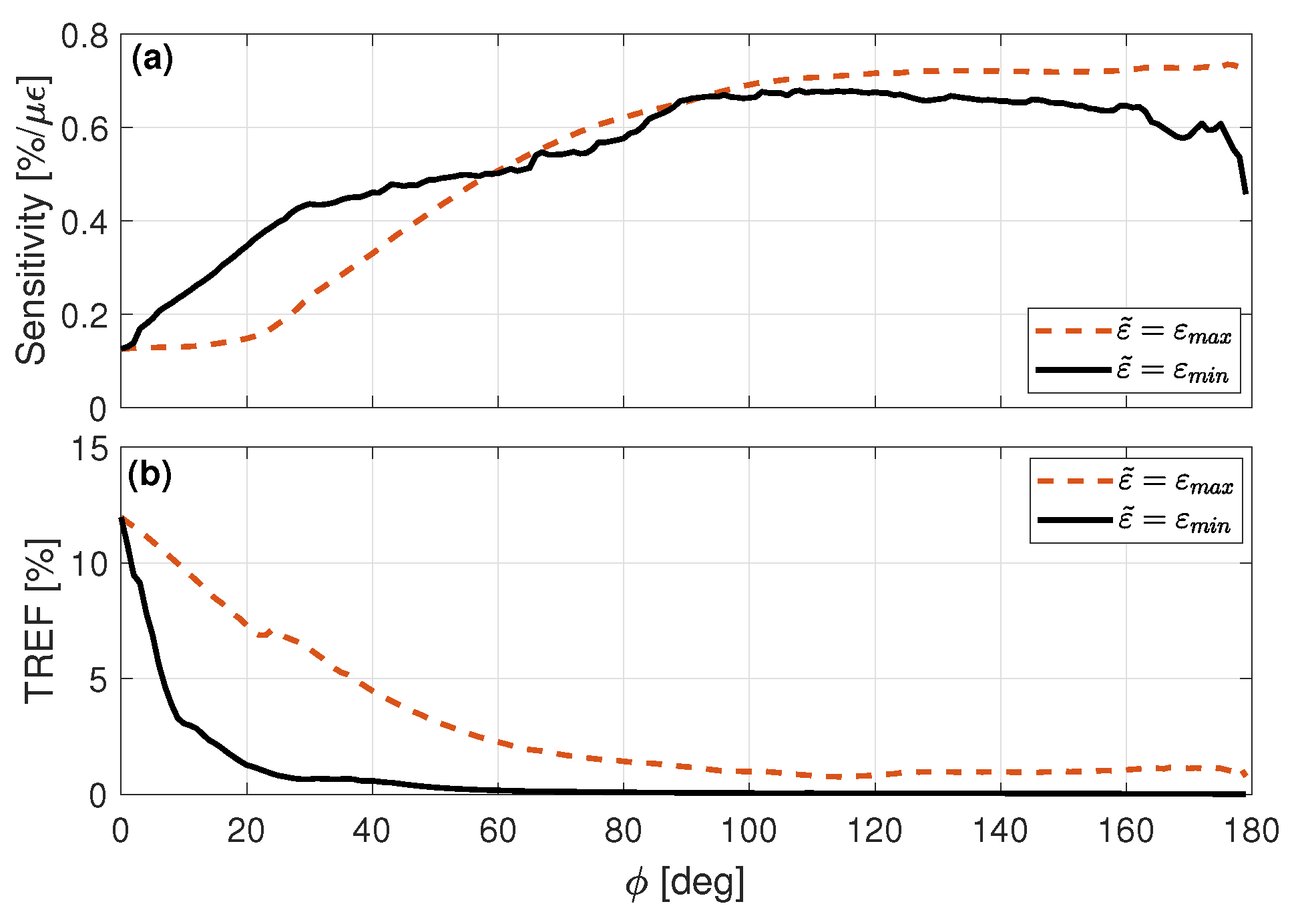
4.3. Dependence on the Reference Strain Level, $\tilde{\epsilon }$

Up to this point, the presented results used the foreknown strain value, $\tilde{\epsilon }$, as the maximum available strain from the experiments, i.e., $\tilde{\epsilon }={\epsilon }_{max}\approx 150 \mu \epsilon$. The proposed technique can, however, use any foreknown strain level. In this section, the effect of taking a different reference strain is evaluated by using a lower value: $\tilde{\epsilon }={\epsilon }_{min}\approx 20\mu \epsilon$.

Figure 14 exemplifies the $M_{\varphi ,\tilde{\epsilon }}(\tau ,f)$ function for the STFT-based filter with $\tilde{\epsilon }={\epsilon }_{min}$ and $\tilde{\epsilon }={\epsilon }_{max}$, where the phase threshold in all cases is $\varphi ={10}^{\circ }$. As can be seen, many fewer components were kept with $\tilde{\epsilon }={\epsilon }_{min}$. This happens because the $\varphi$-sensitive components with lower foreknown strain are actually more sensitive than with a higher reference strain since they present the same amount of phase shifting but relative to a lower strain value. As a consequence, the focused signals $y_{\varphi }(\epsilon ,t)$ obtained with $\tilde{\epsilon }={\epsilon }_{min}$ are expected to be more affected by strain, i.e., more sensitive, than the ones obtained with greater reference strain state. However, as more components are nullified, TREF should decrease more. This behavior can be verified in Figure 15 where the peak sensitivity and TREF as a function of $\varphi$ for the STFT-based filter with $\tilde{\epsilon }={\epsilon }_{min}$ and $\tilde{\epsilon }={\epsilon }_{max}$ are compared. Clearly, the peak sensitivity increases more rapidly with $\tilde{\epsilon }={\epsilon }_{min}$, while TREF becomes virtually zero from about $\varphi ={20}^{\circ }$, which only happens with $\tilde{\epsilon }={\epsilon }_{max}$ from about $\varphi ={70}^{\circ }$.

5. Conclusions

It was possible to identify the frequency components in the reference signal that are most affected by strain through their phase shift compared to a foreknown impulse response under non-zero strain. Then, a filtering procedure was proposed to create a new reference signal without the components that are less sensitive to strain, based on either the Fourier or short-time Fourier transforms. The former analyzes the phase of each frequency component considering the whole signal, whereas the latter considers the phase shift within time-windows. Both filtering techniques implemented in this study were able to increase the sensitivity to strain on the cross-correlated signal. However, an important tradeoff is the decrease of the energy concentration due to the use of the new reference signal.

The STFT-based filter provides a lower decrease of the focusing capability and the sensitivity increased up to about fivefold considering all $\varphi$ range or twice within an interval that does not produce poorly focused signals. The better performance of the time–frequency implementation was due to the ability to distinguish wave packets that arrive at different time instants and share the same frequency, typically found at multimodal and reverberant media, such as the one adopted here. The proposed technique can use in principle any foreknown strain state, $\tilde{\epsilon }$. Here, two values were analyzed, namely low and high strain values. If $\tilde{\epsilon }$ is low, then, for the same threshold angle, the synthesized signal is more sensitive and can produce very low TREF values. Thus, whenever available, a higher strain state should be used since a higher $\tilde{\epsilon }$ makes the technique depend less abruptly on $\varphi$. It is worth highlighting that the need for a foreknown strain state is an intrinsic drawback of the proposed technique. However, the main objective here is to assess whether the sensitivity of the focused signal could be altered and how the proposed procedure is affected by the choice of the parameters and nature of the adopted transform.

The results presented in this paper show that, in reverberant multimodal media, the phase of the signal retains much of the information on the medium strain and that a time–frequency representation is a more suitable analysis tool due to the nature of the signal, which is composed of several waves affected differently by strain and arriving over time with different frequency. The present technique could alternatively be used to analyze the influence of other phase-shifting factors, such as temperature, on the signal components, provided that there are no other relevant sources for phase variation.

References

1. Rizzo, P.; Palmer, M.D.; Scalea, F.L. Ultrasonic characterization of steel rods for health monitoring of civil structures. In Smart Structures and Materials 2003: Smart Systems and Nondestructive Evaluation for Civil Infrastructures; International Society for Optics and Photonics: Bellingham, DC, USA, 2003; Volume 5057, pp. 75–84. [Google Scholar]
2. Xu, J.; Yang, D.; Qin, C.; Jiang, Y.; Sheng, L.; Jia, X.; Bai, Y.; Shen, X.; Wang, H.; Deng, X.; et al. Study and Test of a New Bundle-Structure Riser Stress Monitoring Sensor Based on FBG. Sensors 2015, 15, 29648–29660. [Google Scholar] [CrossRef] [PubMed] [Green Version]
3. Michaels, J.; Michaels, T.; Martin, R. Analysis of global ultrasonic sensor data from a full scale wing panel test. In AIP Conference Proceedings; American Institute of Physics: College Park, MD, USA, 2009; Volume 1096, pp. 950–957. [Google Scholar]
4. Mishakin, V.V.; Dixon, S.; Potter, M.D.G. The use of wide band ultrasonic signals to estimate the stress condition of materials. J. Phys. Appl. Phys. 2006, 39, 4681–4687. [Google Scholar] [CrossRef]
5. Hughes, D.; Kelly, J. Second-order elastic deformation of solids. J. Appl. Phys. Rev. 1953, 92, 1145–1149. [Google Scholar] [CrossRef]
6. Pao, Y.; Sachse, W.; Fukuoka, H. Acoustoelasticity and ultrasonic measurements of residual stresses. Phys. Acoust. 1984, 17, 61–143. [Google Scholar]
7. Mitra, M.; Gopalakrishnan, S. Guided wave based structural health monitoring: A review. Smart Mater. Struct. 2016, 25, 1–27. [Google Scholar] [CrossRef]
8. Gandhi, N.; Michaels, J.E.; Lee, S.S. Acoustoelatic lamb wave propagation in biaxially stressed plates. J. Acoust. Soc. Am. 2012, 132, 1284–1293. [Google Scholar] [CrossRef] [Green Version]
9. Pei, N.; Bond, L.J. Higher order acoustoelastic Lamb wave propagation in stressed plates. J. Acoust. Soc. Am. 2016, 140, 3834–3843. [Google Scholar] [CrossRef] [PubMed] [Green Version]
10. Kubrusly, A.C.; Braga, A.; von der Weid, J.P. Derivation of acoustoelastic lamb wave dispersion curves in anisotropic plates at the initial and natural frames of reference. J. Acoust. Soc. Am. 2016, 140, 2412–2417. [Google Scholar] [CrossRef]
11. Peddeti, K.; Santhanam, S. Dispersion curves for Lamb wave propagation in prestressed plates using a semi-analytical finite element analysis. J. Acoust. Soc. Am. 2018, 143, 829–840. [Google Scholar] [CrossRef] [PubMed]
12. Yang, Y.; Ng, C.T.; Mohabuth, M.; Kotousov, A. Finite element prediction of acoustoelastic effect associated with Lamb wave propagation in pre-stressed plates. Smart Mater. Struct. 2019, 28, 095007. [Google Scholar] [CrossRef] [Green Version]
13. Zuo, P.; Yu, X.; Fan, Z. Acoustoelastic guided waves in waveguides with arbitrary prestress. J. Sound Vib. 2020, 469, 115113. [Google Scholar] [CrossRef]
14. Shi, F.; Michaels, J.E.; Lee, S.J. In situ estimation of applied biaxial loads with lamb waves. J. Acoust. Soc. Am. 2013, 133, 677–687. [Google Scholar] [CrossRef] [Green Version]
15. Pei, N.; Bond, L.J. Comparison of acoustoelastic Lamb wave propagation in stressed plates for different measurement orientations. J. Acoust. Soc. Am. 2017, 142, 327–331. [Google Scholar] [CrossRef] [Green Version]
16. Mal, Y.; Yang, Z.; Zhang, J.; Liu, K.; Wu, Z.; Ma, S. Axial stress monitoring strategy in arbitrary cross-section based on acoustoelastic guided waves using PZT sensors. J. AIP Adv. 2019, 9, 125304. [Google Scholar]
17. Rucka, M.; Zima, B.; Kędra, R. Application of Guided Wave Propagation in Diagnostics of Steel Bridge Components. Archiv. Civ. Eng. 2014, 60, 493–515. [Google Scholar] [CrossRef] [Green Version]
18. Shkerdin, G.; Glorieux, C. Lamb mode conversion in a plate with a delamination. J. Acoust. Soc. Am. 2004, 116, 2089–2100. [Google Scholar] [CrossRef]
19. Kubrusly, A.C.; von der Weid, J.P.; Dixon, S. Experimental and numerical investigation of the interaction of the first four SH guided wave modes with symmetric and non-symmetric discontinuities in plates. NDT E Int. 2019, 108, 102175. [Google Scholar] [CrossRef]
20. Ing, R.K.; Fink, M. Time-reversed lamb waves. IEEE Trans. Ultrason. Ferroelectr. Freq. Control 1998, 45, 1032–1043. [Google Scholar] [CrossRef] [PubMed]
21. Park, H.W.; Sohn, H.; Law, K.H.; Farrard, C.R. Time reversal active sensing for health monitoring of a composite plate. J. Sound Vib. 2007, 302, 50–66. [Google Scholar] [CrossRef]
22. Gangadharan, R.; Murthy, C.; Gopalakrishnan, S.; Bhat, M. Time reversal technique for health monitoring of metallic structure using lamb waves. Ultrasonics 2009, 49, 696–705. [Google Scholar] [CrossRef] [PubMed]
23. Harley, J.; O’Donoughue, N.; Jin, Y.; Moura, J.M.F. Time Reversal Focusing for Pipeline Structural Health Monitoring. In Proceedings of Meetings on Acoustics 158ASA; Acoustical Society of America: Melville, NY, USA, 2009; Volume 8, p. 1. [Google Scholar]
24. Watkins, R.; Jha, R. A modified time reversal method for Lamb wave based diagnostics of composite structures. Mech. Syst. Signal Process. 2012, 31, 345–354. [Google Scholar] [CrossRef]
25. Agrahari, J.K.; Kapuria, S. A refined Lamb wave time-reversal method with enhanced sensitivity for damage detection in isotropic plates. J. Intell. Mater. Syst. Struct. 2015, 27, 1283–1305. [Google Scholar] [CrossRef]
26. Zeng, L.; Lin, J.; Huang, L. A Modified Lamb Wave Time-Reversal Method for Health Monitoring of Composite Structures. Sensors 2017, 17, 955. [Google Scholar] [CrossRef] [Green Version]
27. Kubrusly, A.C.; Pérez, N.; Oliveira, T.F.; Adamowski, J.C.; Braga, A.M.B.; von de Weid, J.P. Mechanical Strain Sensing by Broadband Time Reversal in Plates. IEEE Trans. Ultrason. Ferroelectr. Freq. Control 2016, 63, 746–756. [Google Scholar] [CrossRef] [PubMed]
28. Spalvier, A.; Cetrangolo, G.; Martinho, L.; Kubrusly, A.; Blasina, F.; Pérez, N. Monitoring of compressive stress changes in concrete pillars using cross correlation. In Proceedings of the IEEE International Ultrasonics Symposium (IUS), Glasgow, UK, 6–9 October 2019; pp. 2465–2468. [Google Scholar]
29. Quiroga, J.; Mujica, L.; Villamizar, R.; Ruiz, M.; Camacho, J. PCA based stress monitoring of cylindrical specimens using pzts and guided waves. Sensors 2017, 17, 2788. [Google Scholar] [CrossRef] [PubMed] [Green Version]
30. Kwun, H.; Bartels, K.A. Experimental observation of wave dispersion in cylindrical shells via time-frequency analysis. J. Acoust. Soc. Am. 1995, 97, 3905–3907. [Google Scholar] [CrossRef]
31. Prosser, W.H.; Seale, M.D.; Smith, B.T. Time–frequency analysis of the dispersion of lamb modes. J. Acoust. Soc. Am. 1999, 105, 2669–2676. [Google Scholar] [CrossRef] [Green Version]
32. Niethammer, M.; Jacobs, L.J.; Qu, J.; Jarzynski, J. Time-frequency representation of Lamb waves using the reassigned spectrogram. J. Acoust. Soc. Am. 2000, 107, 19–24. [Google Scholar] [CrossRef] [PubMed] [Green Version]
33. Jeong, H.; Jang, Y.S. Wavelet analysis of plate wave propagation in composite laminates. Compos. Struct. 2000, 49, 443–450. [Google Scholar] [CrossRef]
34. Chen, J.; Rostami, J.; Tse, P.W.; Wan, X. The design of a novel mother wavelet that is tailor-made for continuous wavelet transform in extracting defect-related features from reflected guided wave signals. Measurement 2017, 110, 176–191. [Google Scholar] [CrossRef]
35. Wu, J.; Ma, Z.; Zhang, Y. A Time-Frequency Research for Ultrasonic Guided Wave Generated from the Debonding Based on a Novel Time-Frequency Analysis Technique. Shock. Vib. 2017, 2017, 5686984. [Google Scholar] [CrossRef] [Green Version]
36. Siqueira, M.; Gatts, C.; Silva, R.d.; Rebello, J. The use of ultrasonic guided waves and wavelets analysis in pipe inspection. Ultrasonics 2004, 41, 785–797. [Google Scholar] [CrossRef]
37. Liu, Y.; Li, Z.; Gong, K. Detection of a radial crack in annular structures using guided circumferential waves and continuous wavelet transform. Mech. Syst. Signal Process. 2012, 30, 157–167. [Google Scholar] [CrossRef]
38. Martinho, L.M.; Kubrusly, A.C.; Pérez, N.; Braga, A.M.B.; von der Weid, J.P. Strain sensitivity enhancement of ultrasonic waves in plates using phase filter. In Proceedings of the IEEE International Ultrasonics Symposium (IUS), Glasgow, UK, 6–9 October 2019; pp. 928–931. [Google Scholar]
39. Rose, J.L. Ultrasonic Guided Waves in Solid Media; Cambridge University Press: Cambridge, UK, 2014. [Google Scholar]
40. Zhivomirov, H. On the Development of STFT-analysis and ISTFT-synthesis Routines and their Practical Implementation. TEM J. 2019, 8, 56–94. [Google Scholar]
41. Dodson, J.C.; Inman, D.J. Thermal sensitivity of Lamb waves for structural health monitoring applications. Ultrasonics 2013, 53, 677–685. [Google Scholar] [CrossRef]
42. Lee, S.J.; Gandhi, N.; Michaels, J.E.; Michaels, T.E. Comparison of the Effects of Applied Loads and Temperature Variations on Guided Wave Propagation. In AIP Conference Proceedings; American Institute of Physics: College Park, MD, USA, 2011; Volume 1335, pp. 175–182. [Google Scholar]
43. Bowen, L.; Gentilman, R.; Pham, H.; Serwatka, W.; Fiore, D. Development of 1–3 and 2–2 piezocomposite transducers. J. Acoust. Soc. Am. 1994, 96, 3299. [Google Scholar] [CrossRef] [Green Version]
44. Ferroperm™ Data Sheets from Meggitt Denmar, Meggit Ferroperm. Available online: https://www.meggittferroperm.com/resources/data-sheets/ (accessed on 29 December 2020).
Figure 1. Schematic of the strain monitoring process. In the first step, an impulse-like signal, δ ( t ) , is sent from the transmitting transducer, Tx, and the impulse response of the signal, h ( t ) , is received at the receiver transducer, Rx, which is the reference for the next step. In the second step, the medium is subject to strain, ε , and a new impulse response is obtained. Finally, the impulse responses at both steps, h ( 0 , t ) and h ( ε , t ) , are cross-correlated.
Applsci 11 02582 g001
Figure 2. Schematic of the filtering procedure used to obtain the new ϕ -sensitive reference signal based on the impulse response at some known strain ε ˜ : the overall procedure (a); and a detailed diagram of the filter block (b).
Applsci 11 02582 g002
Figure 3. Experimental setup: (A,B) the transducers; (C) the fixing screws; (D) the threaded rod; (E) the hex nut; and (F) the mounting frame.
Applsci 11 02582 g003
Figure 4. Unfiltered reference signal, h ( 0 , t ) , obtained in the time-domain (a); its FT (b); and its STFT (c).
Applsci 11 02582 g004
Figure 5. Unfiltered focused signal, y ( t ) .
Applsci 11 02582 g005
Figure 6. M ϕ , ε ˜ ( f ) with ϕ = 15 (a) and ϕ = 30 (b) over a narrower frequency band. Note that it assumes values zero or one, according to the phase difference between H ( 0 , f ) and H ( ε ˜ , f ) .
Applsci 11 02582 g006
Figure 7. FT—filtered reference signals in the frequency domain, H ϕ , ε ˜ ( f ) (a,c,e) and in time domain h ϕ , ε ˜ ( f ) (b,d,f), with ϕ = 0 (a,b), ϕ = 15 (c,d), and ϕ = 30 (e,f). Amplitude is normalized with respect to h ( 0 , t ) .
Applsci 11 02582 g007
Figure 8. FT—filtered focused signals with: (a) no filter; (b) ϕ = 15 ; and (c) ϕ = 30 . Amplitude is normalized with respect to y ϕ ( 0 , t ) .
Applsci 11 02582 g008
Figure 9. Peak decrease as a function of strain for FT and STFT filtering. Symbols are experimental measure and lines are their linear fit. Error bar stands for at least five repeated experimental acquisitions at each strain level. Blue symbols and line indicate measurements without filtering ( ϕ = 0 ), red symbols and line indicate reference signal obtained with FT—filtering, and green symbols and line indicate reference signal obtained with STFT—filtering. Both filtering methods were calculated with ϕ = 30 .
Applsci 11 02582 g009
Figure 10. Peak sensitivity (a) and TREF (b) as a function of ϕ for FT and STFT—filtering.
Applsci 11 02582 g010
Figure 11. Time–frequency representation of M ϕ , ε ˜ ( τ , f ) at: (a) ϕ = 15 ; and (b) ϕ = 30 . Black and white spots represent values zero and one, respectively.
Applsci 11 02582 g011
Figure 12. STFT—filtered reference signals in time–frequency domain H ϕ , ε ˜ ( τ , f ) (ac) and in the time domain h ϕ , ε ˜ ( t ) (df), with ϕ = 0 (a,d), ϕ = 15 (b,e), and ϕ = 30 (c,f). Amplitude is normalized with respect to h ( 0 , t ) .
Applsci 11 02582 g012
Figure 13. STFT—filtered focused signals at: (a) no filter; (b) ϕ = 15 ; and (c) ϕ = 30 . Amplitude is normalized related to y ϕ ( 0 , t )
Applsci 11 02582 g013
Figure 14. Time–frequency representation of M ϕ , ε ˜ ( τ , f ) , with (a) ε ˜ = ε m a x and ε ˜ = ε m i n (b), at ϕ = 10 . Black and white spots represent values zero and one, respectively.
Applsci 11 02582 g014
Figure 15. Peak sensitivity (a) and TREF (b) as a function of ϕ with ε ˜ = ε m i n , continuous lines, and ε ˜ = ε m a x , dashed lines, for the STFT—based filter.
Applsci 11 02582 g015