Synchronized Motion Profiles for Inverse-Dynamics-Based Online Control of Three Inextensible Segments of Trunk-Type Robot Actuators

Abstract

This study proposes a novel method for the positioning and spatial orientation control of three inextensible segments of trunk-type robots. The suggested algorithm imposes a soft constraint assumption for the end-effector’s endpoint and a mandatory constraint on its direction. Simultaneously, the algorithm by-design enforces nonholonomic features on the robot segments in the form of arcs. An approximate robot spine curve is the key to the final robot state configuration based on the given conditions. The numeric simulation showed acceptable (less than 1 s) performance for single-core processing tasks. The parametric method finds the best proximate robot state solution and represents the gray box model in addition to existing learning or black-box inverse dynamics approaches. This study also shows that a multiple inverse kinematics answer constructs a single inverse dynamics solution that defines the robot actuators’ motion profiles, synchronized in time. Finally, this text presents rotational expressions and their outlines for controlling the manipulator’s tendons.

1. Introduction

As robotics technology advances, there are more and more efforts to create and control continuum robots that excel in kinematic redundancy. These robots are agile and flexible because of their backbone-less structure, which the biological world has inspired [1,2]. Such robots are called elephant’s trunk or snake-arm robots. This study focuses on three inextensible segments of trunk-type robot’s position and orientation control. Most trunk-type robots are currently used for robotically assisted surgery [3,4], specifically in minimally invasive surgery [5,6]. In the mentioned surgery area, trunk-type robot pose control is crucial, while the continuum robot has to move along a narrow path. This paper presents a control method for trunk-type robots that are more dedicated to tasks requiring robot end-effector spatial control while holding the end-effector position as close as possible to the target. For instance, the authors state that such a concept has the potential to apply continuum robots that are used in urban search and rescue tasks [7], bomb disposal [8], and inspection and repair of aero-engines [9,10]. Continuum robot flexibility and mobility features encourage scientists to look for new kinds of robot-type structure designs and control to adapt robots to other applications.

A continuum robot consists of flexible segments, which, in principle, have a bending motion [1,2]. This bending motion gives two degrees of freedom (DOF) for one section [11]. However, depending on the robot segment type, some segments can also have a linear motion, adding one more DOF. According to this continuum, the robot segment can either have two or three DOF, depending on its type [11,12]. Adding more degrees of freedom to the robot requires additional sections stacked on top of each other. The soft and continuous backbone structure is the main reason why such a multisegment robot is called the continuum. Additionally, continuum robot DOF perfectly describes robot flexibility. For example, it shows that three-segment continuum robots can have between six and nine DOF, which is more than enough for various tasks.

Continuum robots, according to their structure, are divided into three main groups: concentric tube continuum robots [13], pneumatically or hydraulically actuated continuum robots [14], and tendon-driven continuum robots [15]. The concentric tube continuum robot consists of elastic tubes with different diameters. According to their diameter, each elastic tube shoves into the other (starting from the minor tube diameter to the most prominent tube diameter). Pulling these tubes’ ends controls the motion of such a robot. Concentric tube continuum robots primarily operate in surgery because of their small-diameter segments. Pneumatically or hydraulically actuated continuum robots are made of plastic pipes, which usually resemble corrugated pipes in terms of their shape. Compressed air—pneumatic energy, rather than compressed fluid—is the source for these robot types. Pneumatically or hydraulically actuated continuum robots are often used in urban search and rescue tasks. Tendon-driven continuum robot segments consist of spacer disks laid out on the segment elastic backbone (elastic tube). “Tendons” are made of metallic wires and control segments. Tendon-driven continuum robots are utilized primarily in surgery because of the beneficial features of wire usage. However, this specific structure can be adapted not only for the maintenance and repair of aero-engines but also to aid people living with disabilities in completing daily living activities, like an assistive robot [16]. The tendon continuum robot group differs from other continuum robot groups. Its more robust and rigid segment construction gives the continuum robot other technical opportunities to execute particular tasks, such as painting [17].

There are two main segment design variants for the tendon-driven continuum robot: extensible [18,19] and inextensible [20,21]. This study presents the latter. The robot structure designer must know what task a continuum robot is created for and decide how many degrees of freedom a robot needs and how many robot segments there should be. For painting activities, usually, six DOF is enough. Therefore, if continuum robot segments are extensible, the robot has to have at least two segments. In the case of inextensible segments, at least three segments should form a robot. At first glance, it looks like a continuum robot with extensible segments should be a suitable option for painting tasks because this kind of robot will demand fewer materials for robot construction. However, there are other essential characteristics for painting duties, such as robustness and payload. That is why we believe that continuum robots with inextensible segments are preferable to robots with extensible segments. Urniezius’ research showed that the maximum relative entropy principle [22,23,24] could produce closed-form expressions that automatically enforce certain optimization constraints. This study uses numeric application of similar closed-form expressions for an indirect solution to inverse dynamics tasks [25] for a tendon-driven continuum robot. The authors view it as a beneficial tool in black-box-driven inverse dynamics solutions in the future [26].

Now that there is a known continuum robot structure type for painting tasks, a tendon-driven continuum robot with inextensible three segments, the robot actuator control problem emerges. The robot section motors and synchronous actuator motion profiles for the selected robot configuration are discussed towards the end of this study and are the authors’ primary motivation for suggesting trunk-type tendon-driven robot implementation.

The contents of this research paper are as follows. Section 2 is a short review of trunk-type robot kinematics and motion control methods. Section 3 explains the entire approach of a trunk-type robot with three inextensible segments, with an inverse kinematics solution for the imposed end-effector state. This section also discusses tendon length computation, which is necessary for the inverse dynamics part. In Section 4, the simulation results represent the various bending situations of a three-segment continuum robot with end-effector position and orientation errors from the desired target. Section 5 includes robot segments’ motion from the initial position to the target position figures and the electric motor motion profile diagrams.

2. Related Work

The trunk-type tendon robot’s control differs from traditional industrial robots, like Cartesian, cylindrical, polar, and SCARA robots, and from robotic arms or parallel delta robots. The main reason trunk-type tendon control differs from traditional industrial robot control lies in the robot segment construction and motion constraints. While conventional industrial robots utilize rigid links, which move in spatial space with inextensible joints [27], the trunk-type robot does not have rigid links [1,2] but uses a connecting disk (Figure 1). As mentioned before, a trunk-type tendon robot segment spine is usually flexible, and the connecting disk between adjacent segments neither directly causes bending the section nor is used for segment motion. Joints, in this case, serve as connecting pieces in series to get one continuum robot spine (Figure 1).

The only way to control this trunk-type robot is to bend robot segments. Each of the robot segments’ motion is like the arc of a circle, in which the radius is continuously changing while the section is being bent (Figure 2a,b). Knowing this and having a clear view of the robot segment structure sheds light on trunk-type robot design approaches. Some methods implement robot control by using forward kinematics solutions. One example is an operator that directly controls robot actuators via an open-loop user interface [16]. The following example is a robot actuator torque closed-loop control system [28]. Here, the idea is that a robot is used mainly for grasping the object. The robot segment bends around the object and stops when robot actuators produce the same torque as the opposing load torque.

However, there are more trunk-type robot control approaches with inverse kinematics solutions. One proposal is to analyze the trunk-type robot kinematic characteristics with a computer program when the robot’s trajectory end-moving platform is assigned [29]. Then, from model parameters using the spatial backbone modal method, the robot’s kinematic model is established. Nevertheless, the latter method is only valid for hyper-redundant trunk-type robot control. There are also trunk-type robot control techniques where researchers delve into motion planning. One example is the motion planning method for solving the inverse kinematic problems of endoscopic operations of continuum manipulators [30]. The proposed method suggests robot control in a predefined complex environment. Another strategy has the operator control the surgical continuum robot on an arbitrary path in real time and not via a predefined path [31]. The latter paper proposes two-path generation algorithms. One of those algorithms represents an optimization method with sequential quadratic programming. The other algorithm uses differential kinematics with a PID (Proportional Integral Derivative) control algorithm. The robot inverse kinematic model from the joint space to the wire-length space is the basis for these algorithms’ operation.

There is a robot inverse dynamics approach with Euler-Lagrange equations, specifically for trunk-type robots with spherical piezoelectric actuators [32]. In [32], the researchers compared the Euler-Lagrange dynamics method with the analytical potential method. The authors conclude that the latter method is more accurate and efficient than the former.

One of the inverse kinematics methods implements robot control using the modified Denavit-Hartenberg procedure (modified D–H table) and Jacobian matrices using this D–H table [33]. This method relies on the idea that the trunk-type robot segment “is bending with constant curvature”. Consequently, parameters that define each of the robot segments are an outcome of circle arc parameters (the arc length is $L$; the curvature is $k$) and one angle $\phi$, which defines segment orientation around the z-axis (Figure 3a). To improve the D–H method, researchers propose adaptive fuzzy-based fault-tolerant control, as in [6]. The authors claim that their proposed solution significantly reduces position error and increases the robot control reliability.

The circle arc assumption on the robot segment influences most control methods for trunk-type robots [34,35,36]. The main distinctions between these methods are the control approach, the number of sections used, and priorities between end-effector position constraint or end-effector orientation constraint. The latter prioritization is crucial because control algorithms might not necessarily enforce both restrictions due to nonholonomic and dynamics constraints. In this text, the represented method suits a tendon-driven robot orientation with three inextensible segments, and is predefined with determined vector and robot-end positioning control, predefined with point coordinates.

3. Approximate Inverse Kinematics Solution for Imposed End-Effector State

The proposed control method for the position and orientation of a trunk-type robot with three inextensible segments consists of four main steps:

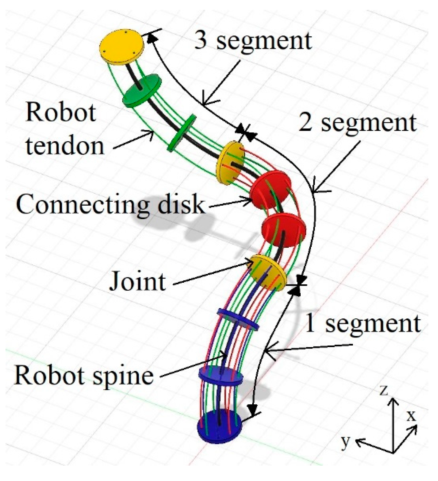
• Trunk-type robot bent spine curve approximation in the 3D Cartesian coordinate system.
• The bending angles ${\theta }_n$ calculation for each robot segment.
• Segments’ endpoints’ x, y, and z coordinates in the Cartesian coordinate system, and sections’ endpoint orientation computation.
• Robot metal wire (tendon) lengths’ calculation according to robot spine curvature and segments’ orientations.

Section 3.1, Section 3.2, Section 3.3 and Section 3.4 explain the above steps in more detail. In the first part, the primary purpose is to get a curve in 3D space such that its length would be equal to the robot spine length, which is predefined and fixed. Here, the soft constraint condition is the goal position, and the mandatory constraint condition is the orientation. The approximate curve endpoint’s orientation must be the same as the preset orientation (as a unit vector). However, the curve endpoint must be as close as possible to the predefined robot’s end-effector point. Then, further calculations will involve estimation of the approximate target position and mandatory target orientation.

In the second and third steps, the top hard constraint condition is that the robot segment shape has to consist of a regular circle arc form. The approximate robot spine will be the prerequisite for the next curve composed of arcs connected in series in these sections. Figure 3a depicts bending angles ${\theta }_n$, segments endpoints $P_n$, and segments orientation ${\widehat{s}}_{\mathrm{orien}n}$ unit vectors found in this approach.

In the final step, the second and third steps’ expressions lead to the estimation of the final segment cables’ lengths. Computed robot tendon lengths are necessary for the robot segment position and orientation control (Figure 3b).

3.1. Determination of Approximate Robot Spine State Configuration

The solution of the three inextensible segments for the continuum robot starts with a consideration of initial conditions. First, the definition of continuum robot spine full-length $l_{\mathrm{r}}$ is necessary. $l_{\mathrm{r}}$ is the sum of all three segments’ lengths $L_n$ (Figure 3a). The three segments’ lengths. $L_1$, $L_2$, and $L_3$, explicitly define the full robot spine length. Point $G$ in 3D space represents the target point that the robot end-effector has to reach. Furthermore, ${\widehat{o}}_r$. defines the desired robot end-effector orientation at the point $G$. Figure 4 depicts all the necessary initial conditions and state.

The robot spine’s length is a fixed-length estimate and should match $l_{\mathrm{r}}$ because the robot segments are inextensible. Knowing this and having information about the preset target point $G$ and orientation ${\widehat{o}}_r$ parametric curve equations are necessary. First, the authors propose an empiric tuning parameter ${\lambda }_{\mathrm{a}}$ and its expression (1) that will play in final spine state expressions:

$${\lambda }_{\mathrm{a}}=\frac{5}{6}\left(-l_{\mathrm{r}}+\frac{\sqrt{k_{\mathrm{r}}\left(l_{\mathrm{r}}^2\left(o_{r\mathrm{x}}^2+o_{\mathrm{ry}}^2+{\left(1+o_{\mathrm{rz}}\right)}^2\right)-24l_{\mathrm{r}}\left( o_{\mathrm{rx}}{x}_{\mathrm{g}}+o_{\mathrm{ry}}{y}_{\mathrm{g}}+z_{\mathrm{g}}+o_{\mathrm{rz}}{z}_{\mathrm{g}}\right)+144{||g||}^2\right)}}{k_{\mathrm{r}}}\right).$$

(1)

Here, $k_{\mathrm{r}}=-31+120v+o_{\mathrm{rx}}^2+o_{\mathrm{ry}}^2+o_{\mathrm{rz}}\left(10+o_{\mathrm{rz}}\right)$. The target point is $G=\left(x_{\mathrm{g}}, y_{\mathrm{g}}, z_{\mathrm{g}}\right)$ (in the Cartesian coordinate system). ${\widehat{o}}_r=\left(o_{\mathrm{rx}}, o_{\mathrm{ry}}, o_{\mathrm{rz}}\right)$ is the unit vector, which defines the robot’s third segment endpoint’s direction. $v$ is a theoretic speed constant ($v = 1$). The trunk-type robot spine’s full length is $l_{\mathrm{r}}$, which equals the sum of all three segments’ lengths. The closed-form expressions for coordinates of point $P_{\mathrm{e}3}$ are contingent upon tuning the coefficient ${\lambda }_{\mathrm{a}}$ expression in Equation (1). Point $P_{\mathrm{e}3}$ expresses the estimated robot spine’s endpoint. The latter point is the closest solution to the target point $G$. Point $P_{\mathrm{e}3}$ coordinates’ equations are necessary for creating estimated robot spine curve parametric equations as functions of time:

$$x_{\mathrm{e}3}=\frac{{\mathsf{\lambda }}_{\mathrm{a}} l_{\mathrm{r}} o_{\mathrm{rx}} + 10 l_{\mathrm{r}} x_{\mathrm{g}}}{12 {\mathsf{\lambda }}_{\mathrm{a}} + 10 l_{\mathrm{r}}},$$

(2)

$${\mathrm{y}}_{\mathrm{e}3}=\frac{{\mathsf{\lambda }}_{\mathrm{a}} l_{\mathrm{r}} o_{\mathrm{ry}} + 10 l_{\mathrm{r}} y_{\mathrm{g}}}{12 {\mathsf{\lambda }}_{\mathrm{a}} + 10 l_{\mathrm{r}}},$$

(3)

$${\mathrm{z}}_{\mathrm{e}3}=\frac{l_{\mathrm{r}} \left({\mathsf{\lambda }}_{\mathrm{a}} + {\mathsf{\lambda }}_{\mathrm{a}} o_{\mathrm{rz}} + 10 z_{\mathrm{g}}\right)}{2 \left(6 {\mathsf{\lambda }}_{\mathrm{a}} + 5 l_{\mathrm{r}}\right)},$$

(4)

$$P_{\mathrm{e}3}=\left(x_{\mathrm{e}3},y_{\mathrm{e}3},z_{\mathrm{e}3}\right).$$

(5)

Finally, Equations (6)–(8) define robot spine curve parametric equations as a function of time, which will define the spine’s curvature:

$${\widehat{x}}_{\mathrm{ec}}\left(t\right)=\frac{t^2\left({\mathrm{x}}_{\mathrm{e}3}\left(-2t+3l_{\mathrm{r}}\right)+\left(t-l_{\mathrm{r}}\right)l_{\mathrm{r}}{o}_{\mathrm{rx}}\right)}{l_{\mathrm{r}}^3},$$

(6)

$${\widehat{y}}_{\mathrm{ec}}\left(t\right)=\frac{t^2\left({\mathrm{y}}_{\mathrm{e}3}\left(-2t+3l_{\mathrm{r}}\right)+\left(t-l_{\mathrm{r}}\right)l_{\mathrm{r}}{o}_{\mathrm{ry}}\right)}{l_{\mathrm{r}}^3},$$

(7)

$${\widehat{z}}_{\mathrm{ec}}\left(t\right)=\frac{t\left({\mathrm{z}}_{\mathrm{e}3}t\left(-2t+3l_{\mathrm{r}}\right)+l_{\mathrm{r}}\left(-t+l_{\mathrm{r}}\right)\left(l_{\mathrm{r}}-t\left(1+o_{\mathrm{rz}}\right)\right)\right)}{l_{\mathrm{r}}^3},$$

(8)

$${\widehat{P}}_{\mathrm{ec}}\left(t\right)=\left({\widehat{x}}_{\mathrm{ec}}\left(t\right),{\widehat{y}}_{\mathrm{ec}}\left(t\right),{\widehat{z}}_{\mathrm{ec}}\left(t\right)\right),$$

(9)

where $t$ represents the time variable, which expresses the spine curve’s trajectory in 3D space (in a 3D Cartesian coordinate system), because curve speed is a constant and is preset to $v = 1$. Equations (10)–(12) represent the robot segment endpoints on a curve as follows:

$${\widehat{P}}_{\mathrm{ec}}\left(t\right)\stackrel{t=L_1}{\to }{\widehat{P}}_{\mathrm{ec}1}=\left({\widehat{x}}_{\mathrm{ec}1},{\widehat{y}}_{\mathrm{ec}1},{\widehat{z}}_{\mathrm{ec}1}\right),$$

(10)

$${\widehat{P}}_{\mathrm{ec}}\left(t\right)\stackrel{t=L_1+L_2}{\to }{\widehat{P}}_{\mathrm{ec}2}=\left({\widehat{x}}_{\mathrm{ec}2},{\widehat{y}}_{\mathrm{ec}2},{\widehat{z}}_{\mathrm{ec}2}\right),$$

(11)

$${\widehat{P}}_{\mathrm{ec}}\left(t\right)\stackrel{t=L_1+L_2+L_3}{\to }{\widehat{P}}_{\mathrm{ec}3}=\left({\widehat{x}}_{\mathrm{ec}3},{\widehat{y}}_{\mathrm{ec}3},{\widehat{z}}_{\mathrm{ec}3}\right),$$

(12)

where the n-th segment length is $L_n$ (in this case, all robot segments are of the same length). The calculated points from Equations (10)–(12) are shown in Figure 5a–c. Point ${\widehat{P}}_{\mathrm{ec}3}$, retrieved using Equation (12), is equal to point $P_{\mathrm{e}3}$, which originates from Equations (2)–(4). Point ${\widehat{P}}_{\mathrm{ec}3}$ is the robot curve endpoint near target point $G$. Figure 5c represents the robot spine curve’s solution.

3.2. Segment’s Bending Angles ${\theta }_n$ Calculation

Computation of an approximate spine curve in Section 3.1 allows for further estimation of each segment’s bending angle. First of all, spine curve parametric equations ${\widehat{x}}_{\mathrm{ec}}\left(t\right),{\widehat{y}}_{\mathrm{ec}}\left(t\right),{\widehat{z}}_{\mathrm{ec}}\left(t\right)$, as in Equations (6)–(8), have first and second function derivatives. Appendix A gives detailed expressions of the computation formulas for ${\dot{x}}_{\mathrm{ec}}$, ${\dot{y}}_{\mathrm{ec}}$, ${\dot{z}}_{\mathrm{ec}}$, ${\ddot{x}}_{\mathrm{ec}}$, ${\ddot{y}}_{\mathrm{ec}}$, and ${\ddot{z}}_{\mathrm{ec}}$. According to [37], Equations (A1)–(A6) are necessary for the evaluation of arc curvature $k$. Equation (13) provides an expression of arc curvature $k$ for a parametrically defined space curve in three dimensions (Cartesian coordinates):

$$k=\frac{\sqrt{{\left({\ddot{z}}_{\mathrm{ec}}{\dot{y}}_{\mathrm{ec}}-{\ddot{y}}_{\mathrm{ec}}{\dot{z}}_{\mathrm{ec}}\right)}^2+{\left({\ddot{x}}_{\mathrm{ec}}{\dot{z}}_{\mathrm{ec}}-{\ddot{z}}_{\mathrm{ec}}{\dot{x}}_{\mathrm{ec}}\right)}^2+{\left({\ddot{y}}_{\mathrm{ec}}{\dot{x}}_{\mathrm{ec}}-{\ddot{x}}_{\mathrm{ec}}{\dot{y}}_{\mathrm{ec}}\right)}^2}}{{\left({\dot{x}}_{\mathrm{ec}}{}^2+{\dot{y}}_{\mathrm{ec}}{}^2+{\dot{z}}_{\mathrm{ec}}{}^2\right)}^{\frac{3}{2}}}.$$

(13)

Inserting Equation (13) into the expression of arc ${\theta }_n=k{L}_n$ returns average bending angles ${\theta }_n$ for any segment based on curvature representations:

$${\theta }_n=\frac{{\int }_0^L\theta \left(t\right)}{t_g}\stackrel{\theta \leftarrow k{L}_n}{\iff }{\int }_0^{L_n} kdt.$$

(14)

The average bending angle ${\theta }_n$ of the n-th segment is one of the main parameters represented in Figure 3a. The following section will present the approach for finding the remaining parameters of the robot segments.

3.3. Calculation of Arc Segments’ Endpoints and Orientations

All three segments’ bending angles ${\theta }_n$ (Equation (14)) and endpoints (Equations (10)–(12)) on the curve allow for finding actual segments’ endpoint coordinates in the Cartesian system. The further derivation will consider robot segments’ shape in an arc form, similar to the ellipse arc seen in the spine curve (Figure 5c). Arc geometry in the x-z plane 2D workspace (Figure 6) allows for obtaining the z coordinates of all three robot segments endpoints $P_n$.

As seen in Figure 6, the triangle $\Delta O{B}_n{P}_n$ will express the coordinate $z_n$, defining a segment endpoint’s z coordinate. Before that, the arc chord length requires determination, for which the formula is

$$d_n=2r_n\sin \left(\frac{{\theta }_n}{2}\right).$$

(15)

Based on circle arc, $r_n$ is equal to

$$r_n=\frac{L}{{\theta }_n}.$$

(16)

Then, the chord length can be expressed as follows:

$$d_n=\frac{2L}{{\theta }_n}·\sin \left(\frac{{\theta }_n}{2}\right).$$

(17)

Triangle $\Delta O{P}_n{C}_n$ (Figure 6) serves for determination of the angle ${\alpha }_n$ that lies between vectors $p_n$ and $c_n$:

$${\alpha }_n=\frac{\pi -\theta }{2}=\frac{\pi }{2}-\frac{{\theta }_n}{2}.$$

(18)

From triangle $\Delta O{B}_n{P}_n$,

$$\sin \left({\alpha }_n\right)=\frac{||e_n||}{||p_n||}=\frac{z_n}{d_n},$$

(19)

$$z_n=d_n\sin \left({\alpha }_n\right).$$

(20)

Substituting $d_n$ and ${\alpha }_n$ from Equations (17) and (18) into Equation (20), its simplification produces $z_n$

$$z_n=\frac{2L \cos \left(\frac{{\theta }_n}{2}\right)\sin \left(\frac{{\theta }_n}{2}\right)}{ {\theta }_n}= \frac{L \sin \left({\theta }_n\right)}{ {\theta }_n}.$$

(21)

Equations (15)–(21) help to estimate coordinates $z_n$ of robot 1, 2, 3 segment endpoints $P_n$. On the other hand, point $P_n$ coordinates $x_n$, $y_n$ can be found similarly to coordinates $z_n$. In this case, all coordinate $x_n$, $y_n$ computations are in the first robot segment coordinate system, around point $O$, (Figure 6). Calculations begin with the estimation of the first segment endpoint’s $P_1$ coordinates, $x_1$, $y_1$.

First of all, vector $p_{\mathrm{ec}1}$ (point ${\widehat{P}}_{\mathrm{ec}1}$ has coordinate estimates based on Equation (10)) has to be normalized so that its magnitude is equal to chord length $d_n$ (Equation (17)). According to [38], the general formula for vector normalization and scaling with a given length is

$$u_{\mathrm{p}}=\frac{l_v{v}_{\mathrm{p}}}{||v||},$$

(22)

where the output vector length is $l_{\mathrm{v}}$, the output vector coordinate is $u_{\mathrm{p}}$ (p stands for x, y, or z), the input vector is $v,$ and the input vector coordinate is $v_{\mathrm{p}}$ (p stands for x, y, or z). According to the generic normalization and scaling formula (Equation (22)),

$$x_{1\mathrm{Norm}}=\frac{{\widehat{x}}_{\mathrm{ec}1} d_1}{||p_{\mathrm{ec}1}||},$$

(23)

$$y_{1\mathrm{Norm}}=\frac{{\widehat{y}}_{\mathrm{ec}1} d_1}{||p_{\mathrm{ec}1}||},$$

(24)

$$z_{1\mathrm{Norm}}=\frac{{\widehat{z}}_{\mathrm{ec}1} d_1}{||p_{\mathrm{ec}1}||},$$

(25)

where the first robot segment chord length is $d_1$. Figure 7, based on Equations (23)–(25), represents a new vector, $p_{\mathrm{Nec}1}$. The magnitude of the calculated new vector $p_{\mathrm{Nec}1}$ is equal to chord length $d_1$. However, the direction in the workspace is the same as the vector’s $p_{\mathrm{ec}1}$ direction:

$$p_{\mathrm{Nec}1}=\left(x_{1\mathrm{Norm}}, y_{1\mathrm{Norm}},z_{1\mathrm{Norm}}\right).$$

(26)

Vector $p_{\mathrm{Nec}1}$ gets new values for its coordinates $x_{1\mathrm{Norm}}$ and $y_{1\mathrm{Norm}}$. Length-invariant direction adaptation of the scaled vector $p_{\mathrm{Nec}1}$ is still necessary. It should rotate in the x-y plane to a new vector $p_1$, which defines the final first robot segment endpoint (Figure 8). To do so, triangle $\Delta O{B}_1{P}_1$ returns the magnitude of $b_1$, as in Figure 6:

$$\cos \left({\alpha }_1\right)=\frac{||b_1||}{||p_1||}=\frac{||b_1||}{d_1},$$

(27)

$$||b_1||=d_1\cos \left({\alpha }_1\right).$$

(28)

Substituting Equations (17) and (18) into Equation (28) and simplifying $b_1$ yields

$$||b_1||=\frac{2L \cos \left(\frac{\mathsf{\pi }-{\theta }_n}{2}\right)\sin \left(\frac{{\theta }_n}{2}\right)}{ {\theta }_n}= \frac{L-L \cos \left({\theta }_n\right)}{ {\theta }_n}.$$

(29)

Normalization of $p_{\mathrm{Nec}1}$ and scaling it to the magnitude $b_1$ produces new $x_1$, $y_1$ values:

$$x_1=\frac{x_{1\mathrm{Norm}}}{||f_{\mathrm{Nec}1}|| }||b_1||= \frac{x_{1\mathrm{Norm}}\left(L-L \cos \left({\theta }_1\right)\right)}{\sqrt{x_{1\mathrm{Norm}}{}^2+y_{1\mathrm{Norm}}{}^2} {\theta }_1},$$

(30)

$$y_1=\frac{y_{1\mathrm{Norm}}}{||f_{\mathrm{Nec}1}|| }||b_1||= \frac{y_{1\mathrm{Norm}}\left(L-L \cos \left({\theta }_1\right)\right)}{\sqrt{x_{1\mathrm{Norm}}{}^2+y_{1\mathrm{Norm}}{}^2} {\theta }_1}.$$

(31)

Combining coordinates $x_1$, $y_1$, $z_1$ enables the expression of the first segment endpoint $P_1$. Then, the segment is in a standard arc form, as follows:

$$P_1=(x_1,y_1,z_1).$$

(32)

The first segment endpoint’s $P_1$ coordinates have already been obtained. Point $P_1$ and bending angle ${\theta }_1$ fully express the robot’s first segment. The segment rotation angle ${\phi }_1$ around the z-axis in Figure 3a is unnecessary. The approach of finding the parameters of the second and third segments will use the quaternion technique. This method requires knowledge of the orientation of the previous segment. In this case, the retrieval of the second segment’s parameters requires knowledge of the first segment’s orientation. Initially, for the calculation of the first segment arc center point $C_1$ (Figure 8a), there is a need to define the circle arc radius with the formula

$$r_1=\frac{L_1}{{\theta }_1}.$$

(33)

Then, point $C_1$ coordinates estimation yields

$$x_{\mathrm{c}1}=\frac{x_1}{||f_1|| }{r}_1= \frac{x_1{r}_1}{\sqrt{x_1{}^2+y_1{}^2} },$$

(34)

$$y_{\mathrm{c}1}=\frac{y_1}{||f_1|| }{r}_1= \frac{y_1{r}_1}{\sqrt{x_1{}^2+y_1{}^2} },$$

(35)

$$z_{\mathrm{c}1}=0,$$

(36)

where $z_{\mathrm{c}1}=0$, because the first segment arc’s center must lie on the x-y axis plane. In Equations (34)–(36), the coordinates all denote

$$C_1=\left(x_{\mathrm{c}1}, y_{\mathrm{c}1},z_{\mathrm{c}1}\right).$$

(37)

Quaternions will allow for estimation of the first segment’s orientation. The calculation starts with finding an axis around which a unit vector defines the first segment orientation rotation. To get this, arc center point $C_1$ needs to be rotated around the z-axis 90° counter-clockwise (Figure 9). The definition of the quaternion’s axis vector is as follows:

$$c_{\mathrm{r}1}=\left(-y_{\mathrm{c}1}, x_{\mathrm{c}1},z_{\mathrm{c}1}\right)=\left(x_{\mathrm{rc}1}, y_{\mathrm{rc}1},z_{\mathrm{rc}1}\right).$$

(38)

By using vector normalization and scaling, as in Equation (22), the vector $c_{\mathrm{r}1}$ magnitude yields a unit vector ${\widehat{c}}_{\mathrm{r}1}$

$${\widehat{c}}_{\mathrm{r}1}=\left(x_{\mathrm{urc}1}, y_{\mathrm{urc}1},z_{\mathrm{urc}1}\right).$$

(39)

Quaternion $q$ expresses rotation around the unit vector axis ${\overrightarrow{OC}}_{um1}$ through the angle ${\theta }_1$, with

$$q=\cos \frac{{\theta }_n}{2}+x_{\mathrm{urc}n}\sin \frac{{\theta }_n}{2}i+y_{\mathrm{urc}n}\sin \frac{{\theta }_n}{2}j+z_{\mathrm{urc}n}\sin \frac{{\theta }_n}{2}k=q_{\mathrm{r}}+q_{in}i+q_{jn}j+q_{kn}k.$$

(40)

For any unit vector that will express first segment orientation and rotation, a rotation matrix $R_n$ exists. This rotation matrix rotates any vector by an angle ${\theta }_n$ counter-clockwise (right-hand rule) by using

$$R_n=\left[\begin{array}{ccc}1-2s\left(q_{jn}^2+q_{kn}^2\right)& 2s\left(q_{in}{q}_{jn}-q_{kn}{q}_{rn}\right)& 2s\left(q_{in}{q}_{kn}+q_{jn}{q}_{rn}\right)\\ 2s\left(q_{in}{q}_{jn}+q_{kn}{q}_{rn}\right)& 1-2s\left(q_{in}^2+q_{kn}^2\right)& 2s\left(q_{jn}{q}_{kn}-q_{in}{q}_{rn}\right)\\ 2s\left(q_{in}{q}_{kn}-q_{jn}{q}_{rn}\right)& 2s\left(q_{jn}{q}_{kn}+q_{in}{q}_{rn}\right)& 1-2s\left(q_{in}^2+q_{jn}^2\right)\end{array}\right],$$

(41)

where the vector’s scalar/real part is $s$, that is $s={||q||}^{-2}$. The quaternion will only rotate the unit vector; therefore, $s=1$. For clockwise rotation around the same axis by an angle ${\theta }_n$, the quaternion rotation matrix is as follows:

$$R_{\mathrm{alt}n}=\left[\begin{array}{ccc}1-2s\left(q_{jn}^2+q_{kn}^2\right)& 2s\left(q_{in}{q}_{jn}+q_{kn}{q}_{rn}\right)& 2s\left(q_{in}{q}_{kn}-q_{jn}{q}_{rn}\right)\\ 2s\left(q_{in}{q}_{jn}-q_{kn}{q}_{rn}\right)& 1-2s\left(q_{in}^2+q_{kn}^2\right)& 2s\left(q_{jn}{q}_{kn}+q_{in}{q}_{rn}\right)\\ 2s\left(q_{in}{q}_{kn}+q_{jn}{q}_{rn}\right)& 2s\left(q_{jn}{q}_{kn}-q_{in}{q}_{rn}\right)& 1-2s\left(q_{in}^2+q_{jn}^2\right)\end{array}\right],$$

(42)

The quaternion formula for vector rotation is

$$v_{\mathrm{r}2}=q{v}_{\mathrm{r}1}{q}^{\prime }=R_n{v}_{\mathrm{r}1},$$

(43)

where the output vector is $v_{\mathrm{r}2}$ and the input vector is $v_{\mathrm{r}1}$. If $v_{\mathrm{r}1}=\left(0,0,1\right)$ then the first segment’s orientation vector is

$${\widehat{s}}_{\mathrm{orien}1}=R_1{p}_{r1}.$$

(44)

The sum of vector ${\widehat{s}}_{\mathrm{orien}1}$ coordinates and point $P_1$ coordinates is equal to $S_{\mathrm{orien}1}$. The vector $s_{\mathrm{orienN}1}$ represents the first segment orientation vector (Figure 10). $s_{\mathrm{orienN}1}$ continues from point $P_1$ to point $S_{\mathrm{orienN}1}$, while the vector $s_{\mathrm{orienN}1}$ magnitude (Figure 10) is scaled up for illustration purposes.

To calculate the second segment endpoint’s $P_2$ coordinates and orientation vector’s $s_{\mathrm{orien}2}$ coordinates, the first segment calculations from Equation (22) to Equation (44) are still valid. However, the second segment vector $p_{\mathrm{ec}12}$ (from point ${\widehat{P}}_{\mathrm{ec}1}$ to point ${\widehat{P}}_{\mathrm{ec}2}$, Figure 5c), from the second segment coordinate system, needs to be transformed into a first segment coordinate system. Therefore, vector $p_{\mathrm{ec}1}$ reduces vector $p_{\mathrm{ec}2}$ to get $p_{\sec 12}$, which starts from point $O=\left(0,0,0\right)$:

$$p_{\sec 12}=p_{\mathrm{ec}2}-p_{\mathrm{ec}1}=\left({\widehat{x}}_{\mathrm{ec}2}-{\widehat{x}}_{\mathrm{ec}1},{\widehat{y}}_{\mathrm{ec}2}-{\widehat{y}}_{\mathrm{ec}1},{\widehat{z}}_{\mathrm{ec}2}-{\widehat{z}}_{\mathrm{ec}1}\right).$$

(45)

Vector $p_{\sec 12}$ needs to be rotated clockwise with the first segment quaternion rotation matrix $R_{\mathrm{alt}1}$ in Equation (42) and using the quaternion rotation formula in Equation (43):

$$p_{\mathrm{ec}2}{}^{\mathrm{T}}=R_{\mathrm{alt}1} p_{\sec 12}.$$

(46)

Vector $p_{\mathrm{ec}2}{}^{\mathrm{T}}$ is a result of the translation to the first segment coordinate system. Figure 11 depicts the $p_{\mathrm{ec}2}{}^{\mathrm{T}}$ vector. Now the second segment chord length $d_2$ allows for scaling vector $p_{\mathrm{ec}2}{}^{\mathrm{T}}$:

$$p_{\mathrm{Nec}2}{}^{\mathrm{T}}=\frac{d_2{p}_{\mathrm{ec}2}{}^{\mathrm{T}}}{||p_{\mathrm{ec}2}{}^{\mathrm{T}}||}.$$

(47)

The estimated vector $p_{\mathrm{Nec}2}{}^{\mathrm{T}}$ lies in the first segment coordinate system. Getting the x-y coordinates requires applying Equations (22)–(44) similarly for the second section. The estimated second segment’s endpoint and its endpoint’s orientation vector exist in the first segment coordinate system (Figure 12).

Translation of the second robot segment endpoint $P_2{}^{\mathrm{T}}$, arc center point $C_2{}^{\mathrm{T}}$, and orientation vector $s_{\mathrm{orien}2}{}^{\mathrm{T}}$ back to the second segment coordination system requires their rotation according to the first segment counter-clockwise quaternion rotation matrix in Equation (41). After that, $P_2{}^{\mathrm{T}}$, $C_2{}^{\mathrm{T}}$ and $s_{\mathrm{orienN}2}{}^{\mathrm{T}}$ add to the first segment endpoint $P_1$. The second robot arc-like segment’s position and orientation are evaluated in the second segment coordinate system (Figure 13).

These second segment calculations apply similarly to the third robot segment. The only difference in this situation is that, in the beginning, vector $p_{\mathrm{ec}2}$ needs to reduce vector $p_{\mathrm{ec}3}$ to get $p_{\mathrm{ec}23}$ ($p_{\sec 23}$), which starts from point $O=\left(0,0,0\right)$. Then, $p_{\sec 23}$ needs to be rotated clockwise with the first segment quaternion rotation matrix $R_{\mathrm{alt}1}$ and then with the second segment quaternion rotation matrix $R_{\mathrm{alt}2}$. For this purpose, similar calculations using Equations (22)–(44) are necessary.

The transposition of the third robot segment endpoint $P_3{}^{\mathrm{T}}$, arc center point $C_3{}^{\mathrm{T}}$, and orientation vector $s_{\mathrm{orien}3}{}^{\mathrm{T}}$ (Figure 14) back to the third segment coordination system is then necessary. These points need to be rotated first with the second segment counter-clockwise quaternion rotation matrix and then with the first segment counter-clockwise quaternion rotation matrix. The third segment endpoint $P_3$, arc center $C_3$ point, and orientation vector $s_{\mathrm{orienN}3}$ add up to the second segment endpoint $P_2$. The third robot segment or robot end-effector position and orientation endpoint vector lie in the third segment coordinate system, as shown in Figure 15.

3.4. Robot Cables’ (Tendons’) Length Calculation According to the Robot Spine Curvature

The key to controlling the shape of a trunk-type robot is cabling (tendons). One trunk-type robot segment can have three or four (or more) tendons dedicated to control. This section will discuss the robot segments’ options with only three cables for the control of each segment. Each segment will have equations for three robot cable lengths $l_{ni}$ (n—segment number, i—cable number).

Some of the cable length formulas originate from [33]. The authors adjusted these equations and used them in the robot control approach. The main reason for choosing these equations was that [33] used robot segment spine curvature and orientation information about robot segment construction. In [33], the equations were based on assumptions that their cables are in straight lines between the section connecting disks and not in the arc-like segment spine. However, the authors of [33] assessed the number of cable guide connecting disks in the section (Figure 16), which is essential for accurate robot cable length calculation.

In [33], the equations for the first segment cable length’s calculation are

$$l_{11}\stackrel{\frac{1}{k_1}=r_1}{\to }{q}_1\left(r_1-D_1\sin {\phi }_1\right),$$

(48)

$$l_{12}\stackrel{\frac{1}{k_1}=r_1}{\to }{q}_1\left(r_1+D_1\sin \left(\frac{\mathsf{\pi }}{3}+{\phi }_1\right)\right),$$

(49)

$$l_{13}\stackrel{\frac{1}{k_1}=r_1}{\to }{q}_1\left(r_1-D_1\cos \left(\frac{\mathsf{\pi }}{6}+{\phi }_1\right)\right),$$

(50)

where the robot first segment cable lengths are $l_{11}$, $l_{12}$, $l_{13}$; the first segment spine curvature is $k_1$; the first segment circle arc radius is $r_1$; the distance from the robot spine center point to the robot cable center point on the robot connecting disk plane of the first segment is $D_1$; ${\phi }_1$ is the angle between a vector ${\widehat{s}}_{\mathrm{orien}1}$ and the first segment coordinate system x-axis on the x-y plane (the angle around the z-axis). The angle ${\phi }_1$ range is $\left[0,2\mathsf{\pi }\right]$ from the x-axis to vector ${\widehat{s}}_{\mathrm{orien}1}$ on the x-y plane in a counter-clockwise direction. $q_1$ comes from this equation:

$$q_n=2m_n\sin \left(\frac{k_n{L}_n}{2m_n}\right)\stackrel{\frac{1}{k_n}=r_n}{\to }2m_n\sin \left(\frac{L_n}{2m_n{r}_n}\right),$$

(51)

where the n-th segment length is $L_n$ and the number of spaces between the connecting disks of the n-th segment is $m_n$. The first robot cable holes’ positions on the connecting disks are necessary to determine the cable lengths for the second and third segments of the robot. Cables conclude three groups: for the first robot segment control $l_{11}$, $l_{12}$, $l_{13}$; for the second robot segment $l_{21}$, $l_{22}$, $l_{23}$, and for the third robot segment $l_{31}$, $l_{32}$, $l_{33}$. According to this, nine cable holes have to be on the robot’s first segment connecting disks, six cable holes have to be on the robot second segment connecting disks, and three cable holes have to be on the robot third segment disks. Punches used for robot cables from the same cable group have to be spaced $120°$ along all connecting disks.

Cable hole positions were first defined in the first segment connecting disks and later on the second and third segment cable guide disks. The starting robot segment cable hole on the first segment guide disk is on the y-axis for first segment control cable $l_{11}$ (Figure 17a). The holes for cables $l_{12}$, $l_{13}$ are placed correspondingly. Disk holes for cables $l_{21}$, $l_{22}$, $l_{23}$ on the first segment are simply the cable $l_{11}$, $l_{12}$, $l_{13}$ holes rotated $40°$ clockwise around point $O$. Furthermore, the cable $l_{31}$, $l_{32}$, $l_{33}$ holes were rotated the same way as $l_{21}$, $l_{22}$, $l_{23}$ but by $80°$. Figure 17a–c depicts all cable hole positions.

Based on the specified hole positions on all robot cable guide disks and Equations (48)–(51) from [36], Equations (52)–(57) for $l_{21}$, $l_{22}$, $l_{23}$ and for $l_{31}$, $l_{32}$, $l_{33}$ cable length expressions are

$$l_{21}=q_1{r}_1+q_2{r}_2-\left(D_1{q}_1\sin \left({\phi }_1+\frac{2\mathsf{\pi }}{9}\right)\right)-\left(D_2{q}_2\sin {\phi }_2\right),$$

(52)

$$l_{22}=q_1{r}_1+q_2{r}_2+\left(D_1{q}_1\sin \left({\phi }_1+\frac{5\mathsf{\pi }}{9}\right)\right)+\left(D_2{q}_2\sin \left({\phi }_2+\frac{\mathsf{\pi }}{3}\right)\right),$$

(53)

$$l_{23}=q_1{r}_1+q_2{r}_2-\left(D_1{q}_1\cos \left({\phi }_1+\frac{7\mathsf{\pi }}{18}\right)\right)-\left(D_2{q}_2\cos \left({\phi }_2+\frac{\mathsf{\pi }}{6}\right)\right),$$

(54)

$$l_{31}=q_1{r}_1+q_2{r}_2+q_3{r}_3-\left(D_1{q}_1\sin \left({\phi }_1+\frac{4\mathsf{\pi }}{9}\right)\right)-\left(D_2{q}_2\sin \left({\phi }_2+\frac{2\mathsf{\pi }}{9}\right)\right)-\left(D_3{q}_3\sin {\phi }_3\right),$$

(55)

$$l_{32}=q_1{r}_1+q_2{r}_2+q_3{r}_3+\left(D_1{q}_1\sin \left({\phi }_1+\frac{7\mathsf{\pi }}{9}\right)\right)+\left(D_2{q}_2\sin \left({\phi }_2+\frac{5\mathsf{\pi }}{9}\right)\right)+\left(D_3{q}_3\sin \left({\phi }_3+\frac{\mathsf{\pi }}{3}\right)\right),$$

(56)

$$l_{33}=q_1{r}_1+q_2{r}_2+q_3{r}_3-\left(D_1{q}_1\cos \left({\phi }_1+\frac{11\mathsf{\pi }}{18}\right)\right)-\left(D_2{q}_2\cos \left({\phi }_2+\frac{7\mathsf{\pi }}{18}\right)\right)-\left(D_3{q}_3\cos \left({\phi }_3+\frac{\mathsf{\pi }}{6}\right)\right).$$

(57)

Here, the robot second segment cable lengths are $l_{21}$, $l_{22}$, $l_{23}$, and the third segment cable lengths are $l_{31}$, $l_{32}$, $l_{33}$. The first, second, and third segments’ circle arc radii are $r_1$, $r_2$, and $r_3$. The distances from the robot spine center point to the robot cable center point on the robot connecting disk plane of the three segments are $D_1$, $D_2$, and $D_3$. The angle ${\phi }_n$ is between vector ${\widehat{s}}_{\mathrm{orien}n}$ and the n-th segment coordinate system x-axis on the x-y plane (the angle around the z-axis).

4. Robot Bending Simulation Results

The authors implemented the represented method equations for a trunk-type tendon-driven robot with three inextensible segments in Wolfram Mathematica (Champaign, IL, USA). Figure 18, Figure 19, Figure 20 and Figure 21 depict the numeric simulation results for multiple simulation scenarios at distinct goal points and robot orientation vectors.

Table 1. Robot technical specifications during the simulations.

Specification	Segment 1	Segment 2	Segment 3
$\mathrm{Segment} \mathrm{length} L_n$ (cm)	40	40	40
$\mathrm{Distance} \mathrm{from} \mathrm{robot} \mathrm{spine} \mathrm{to} \mathrm{the} \mathrm{tendon} \mathrm{on} \mathrm{connecting} \mathrm{disk} D_n$ (cm)	5	5	5

presents trunk-type robot technical specifications that are necessary for simulation execution. The presented robot specifications match the actual robot, which is already in the experimental-practical validation stage.

In this paper, the simulations’ goal is to evaluate the developed method’s efficiency and accuracy. In this case, robot position and orientation errors will express the accuracy of the method. Position error is essentially the scalar Euclidean distance for the robot pose [39]:

$$e_{\mathrm{p}}=||P_3-G||=\sqrt{{\left(x_3-x_{\mathrm{g}}\right)}^2+ {\left(y_3-y_{\mathrm{g}}\right)}^2+ {\left(z_3-z_{\mathrm{g}}\right)}^2}.$$

(58)

Here, the robot third segment endpoint found with the proposed method is $P_3$. The target point that the robot end-effector has to reach is $G$. According to the authors’ decision, the dot product of the third segment orientation ${\widehat{s}}_{\mathrm{orienN}3}$ and predefined orientation ${\widehat{o}}_r$, at the target point $G$, will determine the orientation error. Lipschutz et al. [40] give the mentioned dot product between the two vectors:

$$a·b=||a|| ||b|| \cos \theta ,$$

(59)

where the first vector is $a$ and the second vector $b$ is the angle θ between them. Redesigning the dot product via Equation (59) produces the orientation error expression:

$$e_{\mathrm{o}}= {\cos }^{-1}\frac{{\widehat{s}}_{\mathrm{orienN}3} ·{\widehat{o}}_r}{||{\widehat{s}}_{\mathrm{orienN}3}|| ||{\widehat{o}}_r||}.$$

(60)

Table 2. Robot orientations and position errors as in the simulations in Figure 18, Figure 19, Figure 20 and Figure 21.

Simulation No	Target Point$G$	Reached Point$P_3$	Position Error$e_p$(cm)	Desired Orientation${\widehat{o}}_r$	Reached Orientation${\widehat{s}}_{orienN3}$	Orientation Error$e_o$(°)
1	(87.30, −25, 49.81)	(85.79, −24.33, 51.33)	2.242	(0.94, 0, −0.342)	(0.938, 0.015, −0.346)	0.91
2	(87.30, 25, 49.81)	(85.79, 24.33, 51.33)	2.242	(0.94, 0, −0.342)	(0.938, 0.015, −0.346)	0.9101
3	(−80.30, 27.5, 55.81)	(−82.54, 28.24, 60.01)	4.817	(−0.913, 0.365, −0.183)	($-0.914$, 0.362, −0.183)	0.2195
4	(−74.19, −29.46, 67.64)	(−72.67, −31.09, 64.44)	3.903	(−0.549, −0.768, −0.329)	(−0.567, −0.753, −0.334)	1.3826
5	(50, 0, 63)	(67.21, −1.35, 83.795)	27.028	(0.254, −0.889, 0.381)	(0.289, −0.858, 0.424)	3.617
6	(0, 0, 100)	(5.08, 17.79, 97.99)	18.613	(0.254, 0.889, −0.381)	(0.254, 0.888, −0.382)	0.08424
7	(50, −33, 110)	(47.20, −31.15, 102.41)	8.298	(0, 0, 1)	(0.119, −0.079, 0.99)	8.146
8	(94, −54, 20)	(85.29, −48.46, 26.44)	12.168	(0.651, −0.651, −0.391)	(0.66, −0.634, −0.403)	1.278
9	(55, −55, 80)	(42.36, −42.36, 84.06)	18.325	(−0.615, 0.615, 0.492)	(−0.539, $0.539$, 0.647)	10.658
10	(40, 40, 40)	(53, 53, 37.04)	18.624	(0, 0, −1)	(0, 0, −1)	0

exposes orientation errors between vectors ${\widehat{o}}_{\mathrm{r}}$ and $s_{\mathrm{orienN}3}$ and position errors between goal point $G$ and bent robot third segment endpoint $P_3$. From Table 2, it is clear that the algorithm imposes both constraint conditions: soft for segment goal point and hard for robot end orientation. However, substantial position errors, defined as the distance between desired and achieved robot endpoints, can be seen in some situations, Table 2. For example, the fifth simulation results contain a 27.0281 cm position error. Three main concerns affect the bent robot position accuracy. First, some goal points that have to reach the robot end effector’s target position exceeded the robot’s configuration space. Second, the position error is noticeable because the robot position is soft-constrained, while the primary condition is orientation. Figure 18, Figure 19, Figure 20 and Figure 21 show that reaching the desired locations is possible in most simulations but not with the desired robot end orientations. This is the main reason for the substantial position errors in some cases.

Third, position error results from multiple connected arcs that approximately replace the estimated bent robot spine curve. In most simulations, the spine curve endpoint is closer to the desired goal point, but robot configuration requires arcs as section shapes. Therefore, a minor drift of the spine endpoint is acceptable to impose the segment shape nonholonomic constraint. During this recalculation process, the first task is to get average bending angles ${\theta }_n$ for each arc segment. We assume that the angles ${\theta }_n$ resulting from curvature integration (Equation (14)) must match similar arc sections’ curvature.

Additionally, the lengths of both arc and elliptical curves are the same. However, the chord lengths of arc and elliptical angles are different. The latter explains why position errors between estimated robot spine curves and calculated robot segments arcs endpoints occur in all cases. Only when ${\theta }_n\to 0$ does this position error between the arc and elliptical curve vanish to a minimum.

The authors verified the study routine’s scalability when inverse dynamics problems affect the planning of all robot actuators’ synchronous motion. For this purpose, the authors transformed mathematical scripts into a C program and visually inspected the potential benefits of applying the routines for solving inverse dynamics tasks. A single state (a single target endpoint) spine estimation, (Figure 18, Figure 19, Figure 20 and Figure 21) lasted 200–300 ms on a single core, where the processor had 1.80 GHz, and the RAM was 4 GB. Therefore, the robot control method presented herein is acceptable for both online and offline scenarios. Currently, experimental-practical validation of the three-segment trunk-type tendon robot is ongoing. The authors will reveal research results in the future.

5. Electric Motor Speed Control Profiles

Frequently, an electric motor controls tendon lengths [1,2,5], and such a drive represents a typical actuator. More specifically, electric motors can control trunk-type robot metal wires (tendons) by using Equations (48)–(57) for all three robot segments. Such open-loop (prediction/planning) motion profiles will automatically impose final rigid body motion that practically solves the inverse dynamic problem. That is why this section further elaborates on simulation results dedicated to motor speed control profiles.

First, this study presents angular speed profiles for any generic electric motor installation with or without a gearbox. The only customization parameter value is the radius of a motor rotor or a gear. The parameter helps translate rotational mechanical motion to longitudinal motion, which directly controls a tendon. Accordingly, the speed motion profiles and the kit radii provide an opportunity to plan torque profiles for electric motors and their gearboxes, if any, in the future.

Next, an expression for tendon lengths’ rate of change is necessary to arrive at the angular speed contours. Based on Equations (48)–(57), the approximation of the first-order derivative of cable lengths, as a function of time (Figure 22), is as follows:

$$v_{clnmi}=\frac{\Delta l}{\Delta t}=\frac{l_{nm,i}-l_{nm,i-1}}{\Delta t},$$

(61)

where a cable length $l_{nm}$ belongs to the robot’s n-th segment and its m-th cable, the observation’s discrete-time index is i, and $\Delta t$ is the sampling interval in seconds. Calculating the robot cable length longitudinal speed motor angular speed is then done as follows:

$${\omega }_{nm}=\frac{v_{clnmi}}{r_{\mathrm{ms}}},$$

(62)

where the motor rotor or gear radius is $r_{\mathrm{ms}}$. Motor shaft angular speed also involves the representation of rotational speed:

$${\omega }_{nm}=n_{nm}\left(\frac{2\mathsf{\pi }}{60}\right),$$

(63)

where motor or gear rotational speed is $n_{nm}$, which belongs to the n-th segment and its m-th cable. Combining and simplifying Equations (62) and (63) produces the robot motor shaft rotational speed as follows:

$$n_{nm}=\frac{30v_{clnmi}}{r_{\mathrm{ms}}\mathsf{\pi }}.$$

(64)

The solution of inverse dynamics requires the robot’s end-effector initial state and target state set. The fifth robot simulation (Figure 20a) presents the target $G$ and robot end-effector orientation unit vector ${\widehat{o}}_r$. There are two scenarios discussed that differ in their initial state. The first scenario corresponds to a vertically straight form of the manipulator. The second case will circumscribe the robot as initially bent. Figure 23 and Figure 24 show both situations and their corresponding discrete surfaces that practically represent the inverse dynamics’ numeric solution.

Equations (61)–(64) allow for estimations of speed control profiles in both scenarios (Figure 23 and Figure 24). Simulations involved a radius value of 1 cm for all actuators. The total modeling time for the robot to reach the target position from its initial state was 10 s. Figure 25a,b gives final rotational diagrams of both scenarios that match the cases in Figure 23 and Figure 24.

As in Figure 25, the profile information brings future opportunities for online and offline robot motion planning and prediction when obstacles are present and different trajectory surface configurations come into effect. Simultaneously, these profiles are synchronous, i.e., their open-loop execution will result in final experimental trajectories close to the theoretical solutions proposed by this study.

6. Conclusions

This study proposes an approach for finding synchronized actuator profiles that (by design) solve inverse dynamics problems for a trunk-type robot manipulator consisting of three segments. The intention of the method is the spatial control of the three inextensible segments’ positions and orientations. The technique imposed the soft constraint assumption for the segment’s goal point and the mandatory constraint condition for the end-effector’s alignment. The method’s principle is to obtain an approximate curve of the spatial spine that meets the listed position and orientation conditions. Then, a robot is “built” around the estimated backbone by using circular arcs. The calculated final robot configuration determines all segments’ spatial positions and orientations. The obtained robot configuration also presents all lengths of the corresponding tendons so that their motion implicitly is synchronous. The average time of the code execution varied between 200 and 300 ms.

This study shows that, depending on the specified target point and orientation, the end-effector orientation simulation error ranged from 0° to 10°. Since the robot’s position was not the highest priority in this study, the maximum recorded position error was 27.028 cm and the lowest was 2.242 cm. The total length of the robot’s spine during the simulations was 120 cm. When estimating the error, it is necessary to consider that the authors provide the error statistics regardless of the robot workspace. However, the described method suggested finding the best robot configuration under defined conditions with closed-form expressions, avoiding neural networks [41] or robot motion learning [42] techniques. However, as this work clarifies, the accuracy of the end-effector’s state is the main trade-off.

The approach also presents an approximate discrete inverse dynamics solution relevant for online and offline trunk-type robot motion planning and navigation tasks. This text discusses the rotational profile diagrams for two scenarios. Since the provided motor speed profiles are synchronized, the manipulator’s motion would result in trajectories close to those shown in Figure 23 and Figure 24. The experimental research on a three-segment tendon robot with similar technical specifications to the robot in the simulations is ongoing. The results of this research will appear in the future.

References

1. Li, M.; Kang, R.; Geng, S.; Guglielmino, E. Design and Control of a Tendon-Driven Continuum Robot. Trans. Inst. Meas. Control 2018, 40, 3263–3272. [Google Scholar] [CrossRef]
2. Neppalli, S.; Jones, B.A. Design, Construction, and Analysis of a Continuum Robot. In Proceedings of the 2007 IEEE/RSJ International Conference on Intelligent Robots and Systems, San Diego, CA, USA, 29 October–2 November 2007; pp. 1503–1507. [Google Scholar] [CrossRef]
3. Runciman, M.; Darzi, A.; Mylonas, G.P. Soft Robotics in Minimally Invasive Surgery. Soft Robot. 2019, 6, 423–443. [Google Scholar] [CrossRef] [PubMed] [Green Version]
4. Jha, M.; Ram Chauhan, N. A Review on Snake-like Continuum Robots for Medical Surgeries. IOP Conf. Ser. Mater. Sci. Eng. 2019, 691, 012093. [Google Scholar] [CrossRef]
5. Ouyang, B.; Liu, Y.; Sun, D. Design of a Three-Segment Continuum Robot for Minimally Invasive Surgery. Robot. Biomim. 2016, 3, 2. [Google Scholar] [CrossRef] [PubMed] [Green Version]
6. Piltan, F.; Kim, C.-H.; Kim, J.-M. Adaptive Fuzzy-Based Fault-Tolerant Control of a Continuum Robotic System for Maxillary Sinus Surgery. Appl. Sci. 2019, 9, 2490. [Google Scholar] [CrossRef] [Green Version]
7. Meng, G.Z.; Yuan, G.M.; Liu, Z.; Zhang, J. Forward and Inverse Kinematic of Continuum Robot for Search and Rescue. AMR 2013, 712–715, 2290–2295. [Google Scholar] [CrossRef]
8. Domenech, D.M. New Technologies and Emerging Spaces of Care; ROUTLEDGE: MiltonPark, UK, 2016; ISBN 978-1-138-25006-2. [Google Scholar]
9. Dong, X.; Axinte, D.; Palmer, D.; Cobos, S.; Raffles, M.; Rabani, A.; Kell, J. Development of a Slender Continuum Robotic System for On-Wing Inspection/Repair of Gas Turbine Engines. Robot. Comput. Integr. Manuf. 2017, 44, 218–229. [Google Scholar] [CrossRef] [Green Version]
10. Wang, M.; Dong, X.; Ba, W.; Mohammad, A.; Axinte, D.; Norton, A. Design, Modelling and Validation of a Novel Extra Slender Continuum Robot for In-Situ Inspection and Repair in Aeroengine. arXiv 2019, arXiv:1910.04572. [Google Scholar] [CrossRef]
11. Amouri, A.; Mahfoudi, C.; Zaatri, A. Dynamic Modeling of a Spatial Cable-Driven Continuum Robot Using Euler-Lagrange Method. Int. J. Eng. Technol. Innov. 2020, 10, 60–74. [Google Scholar] [CrossRef]
12. Kang, R.; Guo, Y.; Chen, L.; Branson, D.T.; Dai, J.S. Design of a Pneumatic Muscle Based Continuum Robot with Embedded Tendons. IEEE ASME Trans. Mechatron. 2017, 22, 751–761. [Google Scholar] [CrossRef] [Green Version]
13. Webster, R.J.; Romano, J.M.; Cowan, N.J. Mechanics of Precurved-Tube Continuum Robots. IEEE Trans. Robot. 2009, 25, 67–78. [Google Scholar] [CrossRef]
14. Kang, R.; Branson, D.T.; Zheng, T.; Guglielmino, E.; Caldwell, D.G. Design, Modeling and Control of a Pneumatically Actuated Manipulator Inspired by Biological Continuum Structures. Bioinspir. Biomim. 2013, 8, 036008. [Google Scholar] [CrossRef]
15. Camarillo, D.B.; Milne, C.F.; Carlson, C.R.; Zinn, M.R.; Salisbury, J.K. Mechanics Modeling of Tendon-Driven Continuum Manipulators. IEEE Trans. Robot. 2008, 24, 1262–1273. [Google Scholar] [CrossRef]
16. Coulson, R.; Robinson, M.; Kirkpatrick, M.; Berg, D.R. Design and Preliminary Testing of a Continuum Assistive Robotic Manipulator. Robotics 2019, 8, 84. [Google Scholar] [CrossRef] [Green Version]
17. Webster, R.J.; Jones, B.A. Design and Kinematic Modeling of Constant Curvature Continuum Robots: A Review. Int. J. Robot. Res. 2010, 29, 1661–1683. [Google Scholar] [CrossRef]
18. Frazelle, C.G.; Kapadia, A.; Walker, I. Developing a Kinematically Similar Master Device for Extensible Continuum Robot Manipulators. J. Mech. Robot. 2018, 10, 025005. [Google Scholar] [CrossRef] [Green Version]
19. Nguyen, T.-D.; Burgner-Kahrs, J. A Tendon-Driven Continuum Robot with Extensible Sections. In Proceedings of the 2015 IEEE/RSJ International Conference on Intelligent Robots and Systems (IROS), Hamburg, Germany, 28 September–2 October 2015; pp. 2130–2135. [Google Scholar] [CrossRef]
20. Yeshmukhametov, A.; Koganezawa, K.; Yamamoto, Y. A Novel Discrete Wire-Driven Continuum Robot Arm with Passive Sliding Disc: Design, Kinematics and Passive Tension Control. Robotics 2019, 8, 51. [Google Scholar] [CrossRef] [Green Version]
21. Georgilas, I.; Tourassis, V. From the Human Spine to Hyperredundant Robots: The ERMIS Mechanism. ISRN Robot. 2013, 2013, 1–9. [Google Scholar] [CrossRef] [Green Version]
22. Giffin, A.; Urniezius, R. The Kalman Filter Revisited Using Maximum Relative Entropy. Entropy 2014, 16, 1047–1069. [Google Scholar] [CrossRef]
23. Giffin, A.; Urniezius, R. Simultaneous State and Parameter Estimation Using Maximum Relative Entropy with Nonhomogenous Differential Equation Constraints. Entropy 2014, 16, 4974–4991. [Google Scholar] [CrossRef] [Green Version]
24. Urniežius, R.; Mohammad-Djafari, A.; Bercher, J.-F.; Bessiére, P. Online Robot Dead Reckoning Localization Using Maximum Relative Entropy Optimization with Model Constraints; American Institute of Physics: Chamonix, France, 2011; pp. 274–283. [Google Scholar] [CrossRef]
25. Muller, A. An O(n) -Algorithm for the Higher-Order Kinematics and Inverse Dynamics of Serial Manipulators Using Spatial Representation of Twists. IEEE Robot. Autom. Lett. 2021, 6, 397–404. [Google Scholar] [CrossRef]
26. Watkins-Valls, D.; Xu, J.; Waytowich, N.; Allen, P. Learning Your Way Without Map or Compass: Panoramic Target Driven Visual Navigation. In Proceedings of the 2020 IEEE/RSJ International Conference on Intelligent Robots and Systems (IROS), Las Vegas, NV, USA, 24 October 2020–24 January 2021; pp. 5816–5823. [Google Scholar]
27. Norberto Pires, J. Industrial Robots Programming; Springer: Boston, MA, USA, 2007; ISBN 978-0-387-23325-3. [Google Scholar]
28. Liu, Y.; Ge, Z.; Yang, S.; Walker, I.D.; Ju, Z. Elephant’s Trunk Robot: An Extremely Versatile Under-Actuated Continuum Robot Driven by a Single Motor. J. Mech. Robot. 2019, 11, 051008. [Google Scholar] [CrossRef]
29. Zhao, Y.; Song, X.; Zhang, X.; Lu, X. A Hyper-Redundant Elephant’s Trunk Robot with an Open Structure: Design, Kinematics, Control and Prototype. Chin. J. Mech. Eng. 2020, 33, 96. [Google Scholar] [CrossRef]
30. He, G. Motion Planning and Control for Endoscopic Operations of Continuum Manipulators. Intell. Serv. Robot. 2019, 12, 159–166. [Google Scholar] [CrossRef]
31. Jin, S.; Lee, S.K.; Lee, J.; Han, S. Kinematic Model and Real-Time Path Generator for a Wire-Driven Surgical Robot Arm with Articulated Joint Structure. Appl. Sci. 2019, 9, 4114. [Google Scholar] [CrossRef] [Green Version]
32. Augustaitis, A.; Jurėnas, V. Dynamics of Trunk Type Robot with Spherical Piezoelectric Actuators. IJRA 2020, 9, 113. [Google Scholar] [CrossRef]
33. Jones, B.A.; Walker, I.D. Kinematics for Multisection Continuum Robots. IEEE Trans. Robot. 2006, 22, 43–55. [Google Scholar] [CrossRef]
34. Garriga-Casanovas, A.; Rodriguez y Baena, F. Kinematics of Continuum Robots with Constant Curvature Bending and Extension Capabilities. J. Mech. Robot. 2019, 11, 011010. [Google Scholar] [CrossRef] [Green Version]
35. Neppalli, S.; Csencsits, M.A.; Jones, B.A.; Walker, I. A Geometrical Approach to Inverse Kinematics for Continuum Manipulators. In Proceedings of the 2008 IEEE/RSJ International Conference on Intelligent Robots and Systems, Nice, France, 22–26 September 2008; pp. 3565–3570. [Google Scholar] [CrossRef]
36. Wang, C.; Wagner, J.; Frazelle, C.G.; Walker, I.D. Continuum Robot Control Based on Virtual Discrete-Jointed Robot Models. In Proceedings of the IECON 2018—44th Annual Conference of the IEEE Industrial Electronics Society, Washington, DC, USA, 21–23 October 2018; pp. 2508–2515. [Google Scholar] [CrossRef]
37. Gray, A.; Abbena, E.; Salamon, S. Modern Differential Geometry of Curves and Surfaces with Mathematica, 3rd ed.; Studies in advanced mathematics; Chapman & Hall CRC: Boca Raton, FL, USA, 2006; ISBN 978-1-58488-448-4. [Google Scholar]
38. Urniezius, R.; Giffin, A. Iteration Free Vector Orientation Using Maximum Relative Entropy with Observational Priors. AIP Conf. Proc. 2012, 1443, 182–189. [Google Scholar] [CrossRef]
39. Cohen, D.; Lee, T.; Sklar, D. Precalculus: A Problems-Oriented Approach, 6th ed.; Thomson-Brooks/Cole: Belmont, CA, USA, 2005; ISBN 978-0-534-40212-9. [Google Scholar]
40. Lipschutz, S.; Spiegel, M.R.; Lipschutz, S.; Spellman, D. Vector Analysis and an Introduction to Tensor Analysis, 2nd ed.; Schaum’s outline series; McGraw-Hill: New York, NY, USA, 2009; ISBN 978-0-07-161545-7. [Google Scholar]
41. Wang, Z.; Wang, T.; Zhao, B.; He, Y.; Hu, Y.; Li, B.; Zhang, P.; Meng, M.Q.-H. Hybrid Adaptive Control Strategy for Continuum Surgical Robot Under External Load. IEEE Robot. Autom. Lett. 2021, 6, 1407–1414. [Google Scholar] [CrossRef]
42. Root, K.; Urniezius, R. Research and Development of a Gesture-Controlled Robot Manipulator System. In Proceedings of the 2016 IEEE International Conference on Multisensor Fusion and Integration for Intelligent Systems (MFI), Baden-Baden, Germany, 19–21 September 2016; pp. 353–358. [Google Scholar] [CrossRef]
Figure 1. Three-segment trunk-type tendon robot structure illustration.
Applsci 11 02946 g001
Figure 2. Continuum robot one-segment bending motion: (a) robot segment in a vertical position; (b) the robot segment is bent.
Applsci 11 02946 g002
Figure 3. Continuum robot n-th segment parameters: (a) Robot n-th segment main parameters; (b) robot cables (tendons) view in one segment, robot cables lengths are l 1 , l 2 ,   l 3 .
Applsci 11 02946 g003
Figure 4. Three segments of full-length spine l r (the robot is in the initial position), goal point G , and orientation vector o r   , defined as initial conditions.
Applsci 11 02946 g004
Figure 5. Approximate bent robot spine curve that reaches goal point G and is in vector o r orientation: (a) Preliminary bent robot spine curve first segment; (b) preliminary bent robot spine curve first and second segments; (c) preliminary bent robot spine curve—first, second, and third segments.
Applsci 11 02946 g005aApplsci 11 02946 g005b
Figure 6. Robot segment in the 2D workspace x-z plane (the segment form is in a regular circle arc shape). d n —chord length ( n —segment number); r n —arc radius ( n —segment number); L —circle arc length; O —arc start point; P n —arc endpoint ( n —segment number); C n —circle center point ( n —segment number); A n —middle point of the O P n straight line ( n —segment number); α n —angle between p n and c n vectors ( n —segment number); θ n —arc angle ( n —segment number).
Applsci 11 02946 g006
Figure 7. The first segment vector p ec 1 normalization and scaling to the new vector p Nec 1 : (a) vectors p ec 1 and p Nec 1 with approximate bent robot spine curve view; (b) vectors p ec 1 and p Nec 1 endpoints, zoomed in.
Applsci 11 02946 g007
Figure 8. Robot first segment, when a segment’s form is an arc, endpoint P 1 representation: (a) the point P 1 with approximate spine curve view; (b) points P 1 and P ^ ec 1 , zoomed in.
Applsci 11 02946 g008
Figure 9. First segment vector c 1 rotated around z-axis 90° counter-clockwise.
Applsci 11 02946 g009
Figure 10. First segment with segment endpoint P 1 and with segment’s orientation vector s orienN 1 .
Applsci 11 02946 g010
Figure 11. Second segment vector p ec 2 T calculation representation.
Applsci 11 02946 g011
Figure 12. Second segment endpoint P 2 T and orientation vector s orienN 2 T in the first segment’s coordinate system.
Applsci 11 02946 g012
Figure 13. Second segment endpoint P 2 and orientation vector s orienN 2 in second segment’s coordination system.
Applsci 11 02946 g013
Figure 14. Third segment endpoint P 3 T and orientation vector s orienN 3 T in the first segment’s coordination system.
Applsci 11 02946 g014
Figure 15. Third segment endpoint P 3 and orientation vector s orienN 3 in second segment’s coordination system.
Applsci 11 02946 g015
Figure 16. A trunk-type robot with three segments, each having three tendons.
Applsci 11 02946 g016
Figure 17. Robot cables’ hole positions on the connecting disks: (a) Cables’ hole positions on the first segment connecting disk in the first segment coordinate system; (b) cables’ hole positions on the second segment connecting disk in the second segment coordinate system; (c) cables’ hole positions on the third segment connecting disk in the third segment coordinate system.
Applsci 11 02946 g017
Figure 18. Bent spine views with different endpoint direction unit vector o ^ r (purple vector) and G goal point (redpoint) coordinates’ representation. The light blue curve is an estimated robot spine curve, and the calculated robot segment arc curves are in blue, red, and green: (a) robot spine view when G = ( 87.3016 , 25 , 49.8118 ) and o ^ r = ( 0.9397 , 0 , 0.342 ) ; (b) robot spine view when G = ( 87.3016 , 25 , 49.8118 ) and o ^ r = ( 0.9397 , 0 , 0.342 ) .
Applsci 11 02946 g018
Figure 19. Bent spine views with different endpoint direction unit vector o ^ r (purple vector) and G goal point (redpoint) coordinates’ representation. The light blue curve is an estimated robot spine curve, and calculated robot segments arc curves are in blue, red, and green: (a) robot spine view when G = ( 80.3016 ,   27.5 ,   55.8118 ) and o ^ r = ( 0.9129 ,   0.3652 ,   0.1825 ) ; (b) robot spine view when G = ( 74.187 ,   29.4561 ,   67.6422 ) and o ^ r = ( 0.5488 ,   0.7684 ,   0.3293 ) .
Applsci 11 02946 g019
Figure 20. Bent spine views with different endpoint direction unit vector o ^ r (purple vector) and G goal point (redpoint) coordinates’ representation. The light blue curve is an estimated robot spine curve, and calculated robot segment arc curves are in blue, red, and green: (a) robot spine view when G = ( 50 ,   0 , 63 ) and o ^ r = ( 0.254 ,   0.889 , 0.381 ) ; (b) robot spine view when G = ( 0 ,   0 ,   100 ) and o ^ r = ( 0.254 ,   0.889 ,   0.381 ) .
Applsci 11 02946 g020
Figure 21. Bent spine views with different endpoint direction unit vector o ^ r (purple vector) and G goal point (redpoint) coordinates’ representation. The light blue curve is an estimated robot spine curve, and calculated robot segments arc curves are in blue, red, and green: (a) robot spine view when G = ( 50 ,   33 , 100 ) and o ^ r = ( 0 ,   0 ,   1 ) ; (b) robot spine view when G = ( 94 ,   54 , 20 ) and o ^ r = ( 0.6509 ,   0.6509 ,   0.3906 ) ; (c) robot spine view when G = ( 55 ,   55 , 80 ) and o ^ r = ( 0.6155 ,   0.6155 ,   0.4924 ) ; (d) robot spine view when G = ( 40 ,   40 ,   40 ) and o ^ r = ( 0 ,   0 ,   1 ) .
Applsci 11 02946 g021aApplsci 11 02946 g021b
Figure 22. Tendon lengths’ rate of change profiles for robot segments motion (situation represented in Figure 23) from the initial position to the target position.
Applsci 11 02946 g022
Figure 23. Robot segments’ motion from the initial position to the target position. The light blue curve illustrates the robot spine curve. The calculated robot segment arc curves are blue, red, and green: (a) robot motion side view when the robot is straight in the initial position; (b) robot motion top view when the robot is initially vertically straight.
Applsci 11 02946 g023
Figure 24. Robot segments motion from the initial position to the target position. The light blue curve illustrates the robot spine curve. The calculated robot segment arc curves are blue, red, and green: (a) robot motion side-view, when the robot is bent in the initial position; (b) robot motion top-view, when the robot is initially bent.
Applsci 11 02946 g024
Figure 25. Motor rotational profile diagrams: (a) Motors’ speed profiles when the robot was straight in the initial position, scenario 1; (b) motors’ speed profiles, scenario 2.
Applsci 11 02946 g025