Translating Videos into Synthetic Training Data for Wearable Sensor-Based Activity Recognition Systems Using Residual Deep Convolutional Networks

Abstract

Human activity recognition (HAR) using wearable sensors has benefited much less from recent advances in Deep Learning than fields such as computer vision and natural language processing. This is, to a large extent, due to the lack of large scale (as compared to computer vision) repositories of labeled training data for sensor-based HAR tasks. Thus, for example, ImageNet has images for around 100,000 categories (based on WordNet) with on average 1000 images per category (therefore up to 100,000,000 samples). The Kinetics-700 video activity data set has 650,000 video clips covering 700 different human activities (in total over 1800 h). By contrast, the total length of all sensor-based HAR data sets in the popular UCI machine learning repository is less than 63 h, with around 38 of those consisting of simple mode of locomotion activities like walking, standing or cycling. In our research we aim to facilitate the use of online videos, which exist in ample quantities for most activities and are much easier to label than sensor data, to simulate labeled wearable motion sensor data. In previous work we already demonstrated some preliminary results in this direction, focusing on very simple, activity specific simulation models and a single sensor modality (acceleration norm). In this paper, we show how we can train a regression model on generic motions for both accelerometer and gyro signals and then apply it to videos of the target activities to generate synthetic Inertial Measurement Units (IMU) data (acceleration and gyro norms) that can be used to train and/or improve HAR models. We demonstrate that systems trained on simulated data generated by our regression model can come to within around 10% of the mean F1 score of a system trained on real sensor data. Furthermore, we show that by either including a small amount of real sensor data for model calibration or simply leveraging the fact that (in general) we can easily generate much more simulated data from video than we can collect its real version, the advantage of the latter can eventually be equalized.

1. Introduction and Related Work

Human activity recognition (HAR) using wearable sensors has been a successful research field [1,2] for nearly two decades. There has been the expectation that as large amounts of sensor data become available, HAR will be able to benefit from the advances in Deep Learning techniques in the same way as fields, such as computer vision and speech recognition [3,4]. However, while the application of deep learning methods to HAR has produced undeniable advances [2], the progress has so far been far less significant than computer vision or NLP. Thus for example in recent HAR competitions, most deep learning entries are out-performed by classical machine learning methods, namely random forests [5], while in computer vision, deep learning techniques have dominated since 2012 [6] and beyond [7]. To a large degree this can be attributed to the difficulty of acquiring labeled sensor data from complex realistic scenarios. Consider for example the UCI machine learning repository, a popular machine learning repository. While it contains many datasets for HAR using Inertial Measurement Units (IMUs), their combined volume is less than 63 h, with around 38 of those consisting of simple mode of locomotion activities like walking, standing or cycling. Probably the most popular benchmark datasets in the wearable sensing HAR community are PAMAP2 [8,9] and Opportunity [10,11] with, respectively, less than 8 h of labeled data and less than 14 even if we count all activity granularities. By contrast a well known computer vision repository, ImageNet [12] has images for around 100’000 categories (based on WordNet) with on average 1000 images per category (making it up to 100’000’000 samples). A big HAR related video data set, the Kinetics-700 [13] has 650,000 video clips covering 700 different human activities. With each clip lasting 10 s this is over 1800 h!

There are two main reasons why there are much more image/video data than sensor-based HAR data. First, while more and more people are wearing sensor enabled devices (e.g., fitness trackers) and often uploading to respective platforms, this pales in comparison to those just snapping a picture or making a quick video clip and uploading it to an online repository. Thus, today there are billions of images and videos freely available online, but much less sensor data, even less publicly available. Second, videos can be quickly and easily labeled using crowdsourcing services such as Amazon Mechanical Turk (this is how most ImageNet images were labeled), by leveraging captions, or known topics of image collections. By contrast, labeling sensor data is much more difficult, as interpreting raw sensor data can be challenging even for experts. As a consequence, using crowdsourcing for labeling large amounts of sensor data is not a viable option.

The top level goal of our work is to develop a methodology to allow converting videos of human activities into synthetic sensor inertial measurement unit (IMU) data and thus potentially make all the video based HAR datasets usable for training sensor-based HAR systems.

1.1. Paper Contributions

Recently the idea of using labeled videos to generate “synthetic” sensor data has been proposed as a solution for the HAR training data problem. As one of the first published approaches in this direction we have previously shown [14] initial results on how regression models can be trained to simulate motion sensor data from videos of the respective activities. In that preliminary work we relied on recordings that contained sensor data and videos of the same activities that we later wanted to have the system generate the sensor data for. In this paper, we describe the full development and evaluation of that initial idea making the following contributions:

• We have adapted the method to generalise outside the target exercises. Our model can now be trained on other subjects performing a set of “generic” motions selected to be representative of a broad domain. Using this generic regression model, we can generate synthetic training data for a variety of different activities.
• We have performed and described an in depth analysis of the physical background of deriving different components of the IMU signal and have shown how to simulate different sensor signals beyond acceleration norm.
• We have performed an analysis of the influence of various signal processing techniques on the quality of the simulated sensor signal.
• We have proposed and implemented a new deep neural network based regression model for the generation of simulated sensor data from videos. Compared to our previous work, we now have one regression network per sensor position, which helped reduce overfitting the training motions.
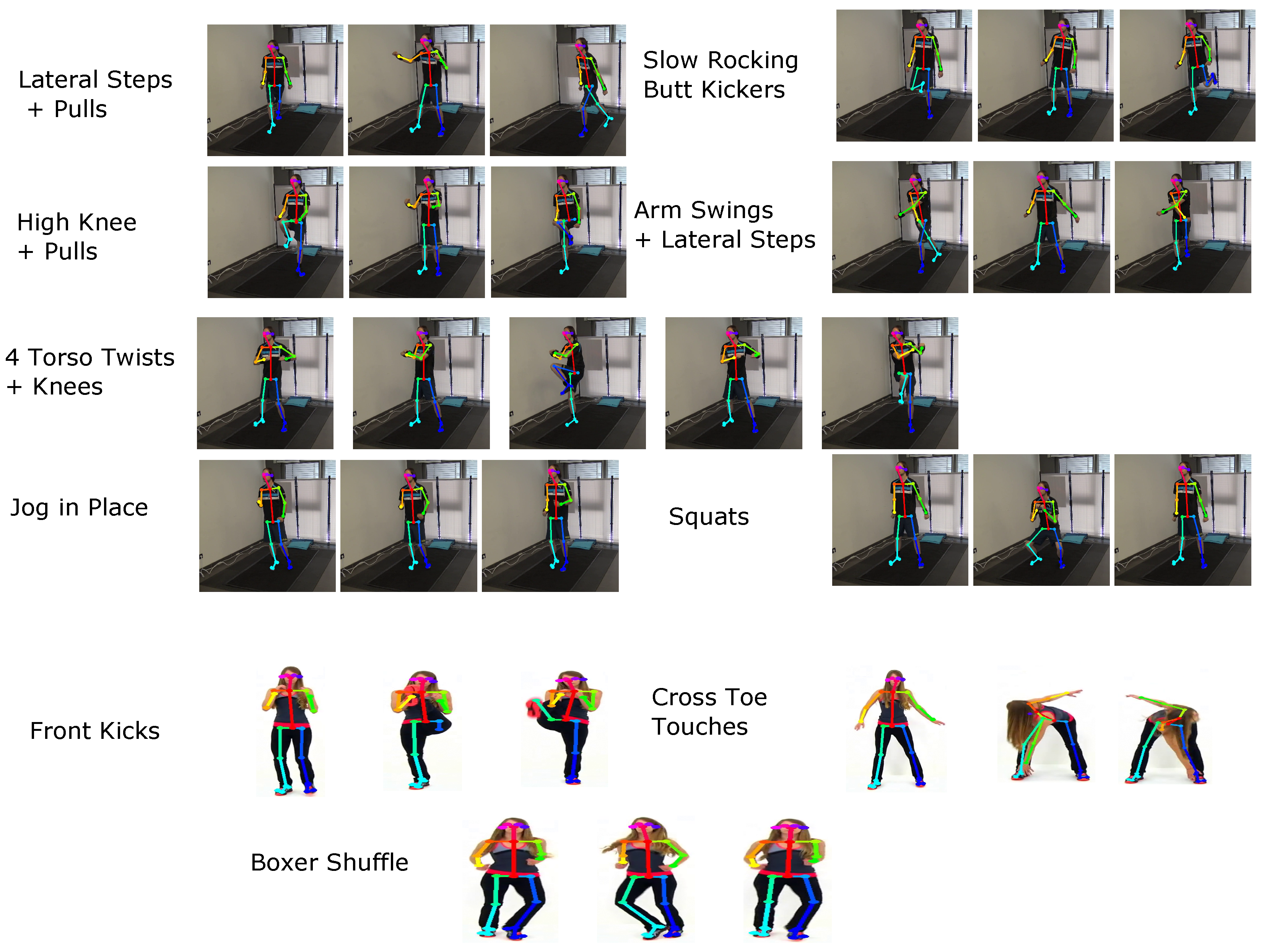
• We have identified a set of generic motions suitable for training the regression model for the broad domain of aerobics like physical exercises, recorded a dataset containing appropriate video footage and sensor data and used it to train the above model.
• We have performed an evaluation on an activity recognition task from the above broad domain of aerobic like exercises for which we have also recorded our own dataset. We have both collected and used as source of simulated training data appropriate online videos. Our analysis includes testing the influence of simulating different sensor modalities and adding small amounts of real sensor data to the simulated one to further improve accuracy. Compared to our previous preliminary work [14], we achieve significantly better results, although the problem that we tackle (using generic motions for training the regression model) is a harder one. Overall we show that

  (a)

  Systems trained on simulated data generated by our regression model and tested on real sensor data can achieve a recognition performance that is within 10% of the recognition performance achieved by a model trained on the corresponding real sensor data.

  (b)

  By increasing the amount of simulated data, we can match the performance of a real signal based model trained on less data. Results so far indicate about a factor of 2 to be needed. This is in line with the motivation behind this work, which is the fact that a very large amount of videos are available for many relevant activities online, which in turn means that we can get much more training data if we can generate it from such videos (which we aim to enable).

  (c)

  Adding even small amounts of real sensor data to fine tune the model generated on the basis of simulated data can improve the performance significantly. In our experiments we found that real data from only 1 or 2 real users can already make the performance of a system trained on simulated data comparable to one fully trained on real data.

Our method for using videos for training sensor-based activity recognition systems follows the steps of Figure 1. First we record a dataset that contains a broad set of generic motions typical for a given domain (e.g., physical exercise). This dataset contains both an appropriate video recording and the corresponding data from on-body sensors. We then train a regression model to map the videos onto the corresponding sensor data. The development of this model is the main contribution of our work. Note that a regression model needs to be generated only one time for a given broad domain. Once it is trained, it can be repeatedly used to generate simulated sensor data for various arbitrary activity recognition tasks from that respective domain. For each new recognition task a set of labeled videos of the respective activities is first acquired (e.g., from YouTube). The videos are then fed to the regression model (step 2) which converts it to simulated sensor data. Obviously the labels for the sensor data are identical to the video labels. Thus we have labeled training sensor data. We next use it to train a recognition model for the required activities (step 3). Finally the trained model is used to recognize those activities from real sensor data in the end application (step 4).

1.2. Related Work

Today in the wearable sensing community there is a broad consensus that obtaining sufficient labeled training data is a key challenge facing the discipline. The use of online information to generate such training data has recently been proposed as a promising approach to address this challenge. While itself not solved and as yet not widely studied, the problem of generation of sensor data from online information sources is closely related to a number of established research fields. These include:

• Simulation of IMU data directly from virtual environments (see Section 1.2.1).
• Generation of 3D animations from 2D monocular videos (see Section 1.2.2).
• Machine learning (ML) methods for generating signal variations such as Generative Adversarial Networks (GANs) (see Section 1.2.3).
• ML methods for predicting signal values in physical systems (see Section 1.2.4).

1.2.1. Simulating IMU Data Directly from 3D Trajectories in Virtual Environments

Many methods exist for simulating IMU data. For example, ref. [15,16,17] provide a simulation environment where one can model human subjects with virtual sensor models to allow experimentation and exploration in virtual space of scenarios in inertial sensing. Depending on the application, specialised tools can be used. For example, there is ample work in simulating foot IMU data for pedestrian dead reckoning [18]. In general many tools exist in this field as simulation is useful for many projects [19,20], but one may also use any existing physical simulator.

While many simulators exist, in general they fail to capture the diversity of human motion and all the different ways different people can perform a given activity. Such diversity can on the other hand be captured by extracting sensor data from videos of real people executing the respective activities as proposed by our work.

1.2.2. Obtaining 3D Poses from Videos

Recently, pose estimation has become a very interesting and successful area of research, with many applications. Obtaining 3D poses is possible with a calibrated system of more than one camera [21]. Commercial systems that can extract poses using 2 cameras (among other things) includes also kinect, which was used in other work [22] to obtain the 3D poses and with it simulate IMU signals. Using a single camera is obviously more challenging. Works in this area include [23,24,25,26,27,28]. Some works [24,27] predict the 2D joints and then fit the 3D skeleton using different strategies, others [23,25,26] are trained to predict 3D joints directly from the image. Even more interestingly, some methods predict both 2D and 3D keypoints [28].

While methods have achieved impressive results, the field is still evolving and the task itself is far from easy due to occlusion, clothing, lighting, and the inherent ambiguity in inferring 3D from 2D [29]. Thus, for the generation of IMU sensor data going directly from 2D poses to IMU, values as proposed by this work is a promising alternative that needs to be investigated.

1.2.3. Deep Learning Based Generation of Signal Variations

While more known in the computer vision community, GANs have shown great promise also in mobile sensors where they have been used to augment datasets and even improve models using semi-supervised learning [30,31]. Those works can generate new sensor data for a specific dataset and label, relying on the data itself and not on the motions of the subject. In other words, in a dataset where we are simulating a person walking, they can generate more data for the sensors available in that dataset, but cannot simulate what the data would be for sensors that were not deployed. This is very relevant as there are many possible sensor placements and possible target activities, and thus being able to simulate, based on the person’s poses, many different placements are necessary, especially if one wants to use online video repositories to obtain sensor data for the target activities. Another case where GANs provide sensor data is through domain adaptation [32], by simulating the readings of one sensor, based on the reading of another one present. While this can alleviate in part the cited restrictions, it requires the source sensor to contain enough information to simulate the target one and is limited to a specific scenario. In the context of poses, GANs have been used to augmented vision datasets by generating subjects in novel poses [33] for better re-identification.

Despite the undisputed potential of the technology, so far there is no work on using GANs to generate sensor data based on video input which is what this work does.

1.2.4. Deep Learning Methods for the Prediction of Physical Parameters

There has recently been increased interest in exploiting the neural networks capability as universal function approximators for the prediction of the dynamics of physical systems, in particular the solution of differential equations [34] replacing traditional methods such as FEMs. Initially, the amount of training data required to accurately model complex physical systems was a problem. As a solution, so called Physically Informed Neural Networks [35] were proposed, which incorporate physical knowledge in the network either as regularisation terms or by leveraging the neural networks automatic differentiation capabilities to capture the information contained in the differential equations.

Obviously, the mapping of poses and pose changes to acceleration and angular velocity values can be seen as a type of physical parameters prediction task where the concept of PINNs can be beneficial. However, so far such an application of the PINN concept approach has not been studied. It is something that we will investigate in future work.

1.2.5. Overall Positioning with Respect to State of the Art

With respect to simulating HAR sensor data, we have [15] doing it directly in simulated environments. Other approaches rely on on-body markers [36,37] or systems with multiple cameras such as kinect [22]. Our approach does not use any special markers, as we would not have access to such markers in video sources such as YouTube. Instead, it relies directly on the position of the body’s joints. Moreover, we do not assume we have more than a single monocular camera, as that is the case for most datasets and video sources. Compared to works using forward kinematics, our approach does not directly perform physical simulation, as it is only feasible if the 3D poses of the subject are estimated. Obtaining those 3D poses is possible with a calibrated system of more than one camera [21] or even using a single one [23,24,25,26,27,28]. Thus, one could extract those poses and then use the cited methods to obtain the sensor values, but their quality depends on the quality of poses that can be obtained from a monocular camera. Recent work that follows this approach is [38], which uses off the shelf methods to predict 3D human poses for monocular images and then forward kinematics to simulate sensor data. They have demonstrated the feasibility of the approach in generating acceleration data without a static camera, but their pipeline works best when predicting modes of locomotion and not complex activities that do not happen in a 2D plane [38]. This is likely due to accumulated distortions in the predicted 3D poses. Extracting those poses from a monocular camera is no easy task due to occlusion, clothing, lighting, and the inherent ambiguity in inferring 3D from 2D [29]. Our approach is different as we predict sensor data directly from the 2D poses using a deep neural network without forward kinematics or a complex pipeline that includes several deep neural networks. We situate our work in the area of applying advances in vision to the HAR field. More recently vision has been shown to be successful for both labeling and knowledge transfer in mobile sensor-based HAR [39], indicating that there are many benefits in using video information too for HAR and many cases where it can aid in data acquisition.

2. Problem Description and Design Considerations

A video (at least when taken from the right perspective) clearly contains elaborate motion information. On the other hand, signals produced by the sensors that we are considering (IMUs and their components: accelerometers and gyroscope) are in effect a representation of motion. The generation of IMU signals from known 6DOF (x,y,z coordinates plus the yaw, roll pitch angles) trajectories is a well understood and solved task. Thus in simplified terms we consider the mapping from one representation of relevant motion (video) to another (IMU sensors). The difficulty that we need to address stems from three considerations:

• Fundamental incompleteness of 2D video information. Monocular video (which is what we need to work with to be able to harvest online video sources) does not contain complete 6-DOF information about objects (in our case human body parts) that it shows. Instead for each object a single video frame provides 2D coordinates in its own frame of reference which are essentially the x- and y-coordinates in pixels. When looking at such a frame humans can translate such 2D image coordinates into information about physical coordinates (which in some cases may include all 6 DOFs) through semantic analysis of the picture and putting the results of such semantic analysis in the context of their understanding of the world. Thus when seeing a man waving his arms, we can estimate the physical coordinates of various body parts with respect to each other just from our knowledge of human physiology (degrees of freedom of joints, typical motions typical size and proportions of human body etc.). Clearly not knowing the exact dimensions of the specific person, this can only be an approximation.
• Inherent inaccuracies in 2D video information. Even when physical coordinates of relevant body parts can in principle be inferred from the semantic information, the achievable accuracy can vary greatly depending on the camera angle and position. Thus, for example, given frontal view of the user (as for example in Figure 2 the x-y position of the wrist, which is point 4 in Figure 3) in respect to the hip (point 8) can be estimated with reasonable accuracy. On the other hand, the angle of rotation of the wrist around the lower arm axis is much more difficult to estimate accurately. This is because in a typical video, the wrist itself can be just a few pixels wide.
• Sensor specific physical effects. Sensor signals are influenced by factors which do not directly manifest themselves in an image. Best example of this is gravity. While the direction of “down” can mostly be inferred from semantic analysis of an image, it is not always enough. Consider the example of the wrist rotation above in the context of a wrist worn acceleration sensor. If the lower arm is parallel to the ground then the rotation determines how the gravity vector is projected onto the sensor axis perpendicular to the lower arm. Thus, the rotation has a very significant influence on the value of the acceleration signals on those two axes. On the other hand, as described above, wrist rotation tends to produce a “weak signal” in an image so that it can only be roughly estimated. Another example is high frequency “ringing” of the acceleration signals, when for example the user stamps his feet on the ground. This results from high frequency vibration of the device caused by the strong impact of the foot on a hard surface and is a very characteristic feature in the acceleration signals, but mostly invisible on the video signal as the amplitude of the vibration is too small and affects the device only (not body parts as a whole) which may be invisible (e.g., hidden under clothing).
• Frame of reference and scaling. IMUs typically use the “world” coordinate system which relies on magnetic sensors to determine geographic north and derives the direction of the gravity vector as down. The signals are given in standard units (e.g., $\frac{m}{s^2}$ for acceleration). In principle gravity can be derived through semantic analysis of an image, which is however not necessarily trivial and not always reliable. Obviously in most images "north" is not given. All motions are given in pixels per frame with the relationship between pixels and physical units depending on the camera position and settings. Overall the translation between the image frame of reference and pixel units and the sensor frame of reference and physical units is a non trivial challenge, even more in videos obtained from online repositories where cameras are not calibrated.

In summary the generation of IMU sensor data from videos cannot be accomplished with an exact physical model. This is a fundamental difference to the well understood and largely solved problem of generating IMU values from 6DOF trajectories. Instead a heuristic approach is needed that minimizes the unavoidable errors with respect to the needs of a given domain. Here a key question is whether we narrowly optimize the system to a specific domain or follow a more general domain agnostic approach. Other core design concerns are how much, at which stage in the process and in what form can physical models be included and what they can accomplish and which part of the task will be delegated to what type of data driven ML approaches. The most obvious choice is between (1) using existing ML methods for estimating 3D poses from 2D videos [23,24,25,26,27] and then using bio mechanical models [15] to generate the sensor data and (2) training an end-to-end ML model that goes directly from 2D video to sensor data. For the ML approach (this work), questions include how to accomplish the conversion between image frame of reference and pixel coordinates, how to handle the sensor frame of reference and its physical units and whether to explicitly filter, scale and normalize the signal.

3. Method

In this section we will explain in detail our method starting with how it is trained, which is shown in Figure 4. The first training step consists of extracting the poses from video and translating them into appropriate parameters:

• The application of standard tools (specifically Open Pose [21,41]) to identify humans in videos and extraction of their 2D poses. The poses are defined in terms of joint coordinates in pixels.
• Optional: low pass filtering.
• A sliding window based translation of the raw 2D pixel coordinates into appropriately filtered and scaled values in the body centered (hip as origin) frame of reference. This window considers $1.5$ s in the past and $1.5$ in the future, with a total length of 3 s.
• Generating sliding windows of the pre-processed pose data with window size W and step S.

The system is trained on a dedicated dataset that contains synchronized sensor and video data for a set of motions typical for a broad domain. The sensor data collected is used as ground truth for training the regression model. Thus, any pre-processing of the sensor data performed before it is used to compute the loss will be reflected in the synthetic sensor data that the model will learn to generate. This means that the aim of the pre-processing must be to remove from the sensor signal any information that will hamper learning by “confusing” the model (noise, frequencies too high to be contained in the video data), while retaining as much useful information as possible. Examples of pre-processing strategies that we investigated were low pass filtering with different cut off frequencies and scaling. After pre-processing we aggregate the ground truth sensor data into sliding windows with window size W and step S to correspond to the partitioning of the pose parameters. The sliding windows are the input to the regression model. After some experimentation we have settled on a model based on residual deep convolution neural networks that uses dilated convolutions, similar to a Temporal Convolutional Network (TCN) [42]. We train a separate model for each sensor position and channel. Once trained, the system is presented with a video of the activity and produces a corresponding sequence of simulated sensor signals.

In the remainder of this Section we will explain in detail the training steps of our method. In Section 3.1 we go into depth about how we obtain poses for each video as well as explain the procedures and rationales behind our sensor and pose pre-processing. The motivation and configuration of our deep learning model is explained in Section 3.2, while the dataset that was used to train it, is described in Section 3.3.

3.1. Obtaining 2D Poses

We used the OpenPose library [21,41] to extract 2D poses of subjects in each frame. The poses are given in terms of rigid body segments connected by respective joints as shown in Figure 3. We accept all joints detected by OpenPose with at least 0.0002 confidence. We track each subject in a video using their Mid Hip coordinates. For each subject, missing joints are filled using linear interpolation. This is done for two reasons: First, not all joints are detected in all frames. Second, videos vary in fps, so we reach 50 poses per second after linear interpolation. This is used for all video sources as the target YouTube videos we used vary in fps from 24 to 60, but the training ones we recorded had 50 fps.

3.1.1. Pose Translation and Processing

For every video frame the pose extraction system produces the pixel coordinates of the individual joints (and/or the angles between the respective rigid body segments). The values depend not only on the motion of the user, but also on the camera perspective. The same posture at the top left corner of an image will produce different coordinate values than at the bottom right. For a given motion the position difference between two frames expressed in pixels will be different when executed close to the camera than when executed far from the camera (and will also vary depending on the angle and of course the resolution of the video). On the other hand the sensor values that we want to generate are expressed in absolute physical units and are related only to the user action (and of course sensor placement on the body). In summary we need to address (1) the translation of the poses into coordinates that are independent of the position of the user in the image and (2) a scaling making the magnitude of pose changes between frames invariant with respect to the size of the user’s body in the image. Given the power of modern deep learning based computer vision systems one could in principle attempt to have the system learn the corresponding transformation from data. However, this would require a very large amount of data on top of the data needed to learn the dependence of the motions observed in the video and the sensor signals as such. As a consequence our method contains an explicit pre-processing step before feeding the data into the regression model.

As a scaling factor to achieve motion amplitudes independent of the distance from the camera we use body dimensions in the picture. In other words we express the magnitude of motions in “units” of body size as seen in the image. To this end we selected the euclidean distance between Neck and MidHip (joints 8 and 1 in Figure 3) as a scaling factor for the motions expressed in pixels. Since the distance between the camera and the user can change we recompute the scaling factor for every frame. Let’s call the euclidean distance at time t the $dis{t}_t$. In order to avoid scaling outliers, we are going to use a sliding window of size 3 s, $1.5$ back and $1.5$ forward, and compute the median. This value we call the $scal{e}_t$ which is

$$scal{e}_t=median(dis{t}_{t-75},\dots ,dis{t}_{t+75})$$

(1)

and the function to scale any value $v_t$ is

$$scale(v_t,scal{e}_t)=-1.0+\frac{v_t}{scal{e}_t}\ast 2.0$$

(2)

We represent the joint position in a frame of reference centered in the MidHip joint, that is, joint 8 in Figure 3. This means that for each joint other than the MidHip we compute its new x coordinate at time t ($NewJoin{t}_x^t$) and y coordinate at time t ($NewJoin{t}_y^t$) using

$$\begin{array}{c}\hfill NewJoin{t}_x^t=scale(Join{t}_x^t-MidHi{p}_x^t,scal{e}_t)\\ \hfill NewJoin{t}_y^t=scale(Join{t}_y^t-MidHi{p}_y^t,scal{e}_t)\end{array}$$

(3)

This provides us with a coordinate system that is independent of the location of the person in the image. Note, that a single scale is used for both x and y, as the aim is to match real space and not to do standard machine learning scaling. In other words, the scale translates pixel distances to joint relative ones, so it should be the same for both axes in order to not deform the poses.

For the MidHip joint we do not perform this procedure, as all joints are now relative to it. In order to capture the overall movements of the human in the picture plane (which can have influence on the acceleration values), we also include the scaled x and y speed of the MidHip, which means adding to our input

$$\begin{array}{c}\hfill HipSpee{d}_x^t=scale(MidHi{p}_x^{t+1}-MidHi{p}_x^t,scal{e}_t)\\ \hfill HipSpee{d}_y^t=scale(MidHi{p}_y^{t+1}-MidHi{p}_y^t,scal{e}_t)\end{array}$$

(4)

Using joint positions relative to MidHip also obscures motion of the body towards and away from the camera and its influence on the sensor signals. Fortunately, we can retrieve this information by giving the model access to two extra values related to the $scal{e}_t$ representing the relative speed of scale change

$$spee{d}_t=\frac{scal{e}_{t+1}-scal{e}_t}{scal{e}_t}$$

(5)

and the first derivative of this scale speed. To distinguish between the camera moving and the motion of the user in the environment, we can consider the optical flow within the picture as a whole (which we do not do yet as in our sample data the camera was static). As we explained, changes in scale can be a proxy for absolute movement as the subject is coming closer to/moving away from the camera regardless of specific initial coordinates.

3.1.2. Additional Signal Processing and Selection

Signal processing beyond the translation and scaling of the features described above can be considered in two categories. The first is further improvement of the quality of the pose information extracted from video. Here, smoothing of the scaling using the median to remove small shifts in joint position and removing outliers in cases where the network predicts a distorted pose in some of the frames have proven to be most effective. Note that these steps are applied to the video signal only. With respect to the sensor signal, the only prepossessing we have found to be consistently effective was linear interpolation of the sensor data to 50 Hz to match the video frame rate.

The second is the removal from the signal of components that are unlikely to be reliably translated from video to sensor signals (see also Section 2). In essence the idea is to entirely remove certain types of information from our classification process, opting to have less, but more reliable information. Examples are: computing the norm of 3D sensor signal. gravity removal (“linear acceleration”) and low pass filtering. The latter was motivated by the insight (see Section 2 point 3) that phenomena such as high frequency “ringing” of the signal caused by sudden, strong impacts that are fundamentally invisible in the video data. This means that the simulated sensor data generated from videos will not contain such “ringing”.

These steps need to be applied to both the sensor signals and the video signals and done during: the training of the regression model, the generation of the synthetic training data, and the classification of real sensor data with the model generated using the simulated data. Obviously, in cases where the information is not present in the video signal at all, it is sufficient to remove it from the sensor.

3.2. Regression Models

As regression model we selected a residual deep convolutional neural network that uses dilated convolutions, similar to TCN [42]. It has been shown to be successful in many sequence modeling tasks, outperforming even long short-term memory models [42]. Our architecture (Figure 5) relies on dilated convolutions and residual connections present in the TCN blocks. Residual connections help train deeper networks by adding the output of convolutions to an identity function [43], while dilated convolutions increase the receptive field by orders of magnitude without increasing the computational cost. By employing the same padding in all convolutions, we maintain the temporal size of the inputs, allowing us to go deeper even when using small temporal windows and map the sequence of poses to the sequence of sensors signals. In order to prevent overfitting, we apply dropout in all TCN blocks except the first and reduce the number of parameters by decreasing the number of filters in the 4th TCN block by applying convolutions with filter size 1. We train one regression model per sensor position and feature. Each model was trained using the mean squared error loss and the Adam optimizer [44] with $0.001$ learning rate and $0.9$ and $0.999$ for ${\beta }_1$ and ${\beta }_2$, respectively. The model was trained for 500 epochs with early stopping using a patience of 25 to avoid overfitting.

It is important to discuss the motivation for our training regimen. A key question for the training is which information from the video to include in training which sensor.

• Providing information about the motion of body parts that we know, from physical consideration, to be irrelevant for the signal of a given sensor at a given location will “confuse” the model. Eventually, given enough data, good models will likely learn to distinguish relevant from irrelevant information. However, getting rid of confusing information is known to significantly reduce the amount of required training data and speed up training.
• Providing information about body parts that, from a bio-mechanical point of view do not influence each other, on the other hand can be counterproductive and lead to overfitting the specific training motion sequences and combinations. As an example, consider the motion of the left and right wrist. With the exception of some very extreme motions (e.g., extremely strong shaking of one wrist making the whole body shake), the motion of one wrist has no influence on the other. However, in many motion sequences there are sometimes strong correlations between the motion of both wrists. The best example is walking when people often swing their arms in sync. When training the system to recognize walking, we want the system to learn such correlations. However, when training a regression that should map motions in an image onto sensor data for arbitrary activities based on physical constraints only this would be undesirable overfitting of artefacts of the specific training sequence.
• Finally there is the question if a joint model should be trained for all sensor signals, if separate models should be trained for all signals from one on-body location or if we should train a separate model for each signal at each location. Training one model for all locations and signals is not advisable due to the need of avoiding overfitting a specific training set because of spurious correlations between signals from different locations. In principle, training a model to generate all the signals from a given body location should allow it to capture the physical dependencies between those signals and should thus improve the quality of the results. However, in our experiments we have found individual models trained for each sensor modality at each location to perform best. This may be due to insufficient training data. It may also be necessary to introduce onto the model mechanisms for explicitly encoding physical boundary conditions as proposed, e.g., by the concept of Physically Informed Neural Networks [45].

For each target sensor signal we trained one regression model per possible sensor placement using only the joints relevant for it. We placed sensors on the wrists and calves, as shown in Figure 3, which also shows which joints are used for each position. For each one of those inputs we built a regression model as depicted in Figure 5. Regression is done using a window of size 16 frames (around a third of a second) and step 1. This increases training data and was also selected to avoid overfitting specific movements. The regression output is 16 numbers representing the IMU values for one channel at those times. The input for each regression model using $n_j$ joints is a tensor $(16,n_j+2,2)$, that is, the 2D coordinates of the joints involved and also the 2 extra values related to the scale changes and hip speeds mentioned earlier. For the joints involved for each position, see Figure 3.

3.3. Datasets for Training the Regression

Our aim is to train a model that can generate simulated sensor data not just for a single specific set of activities but for a broader domain. Thus having our regression model, application developers should be able to use our model to generate the required training data from online videos for any activity set they are interested in (as long as it is within the broad general domain). The idea is thus to train the regression model on a set of motions that are representative “basic components” of the activities of the respective broader domain. The core question is how to define the “broader domain” and how to identify the corresponding “basic components”. For this work we have selected aerobic-like physical training. It is a very broad domain with a great variety of different exercises for which online videos are extremely popular. In terms of applications the ability to monitor the exercises is something that current fitness trackers lack, despite the popularity of such exercises and the associated potentially large user base. In technical terms the domain has the advantage that the corresponding videos tend to provide a stable, easy to process frontal perspective with the relevant parts being clearly visible most of the time (as the whole purpose of the videos is to show the viewers how to move). The activities tend to be characterized by distinct motion of the limbs and posture changes which means that recognition systems should be reasonably robust with respect to sensor data noise and inaccuracy.

With respect to the “basic components” of the motions we first started by showing the participants example videos of the domain and asking them to perform random motions related to those videos. This approach has not produced good results, however, as people tended to repeat the same, not necessarily representative motions. We then turned to high school video material explaining the degrees of freedom of human joints and the types of motions that different muscles can actuate. We combined parts of 7 such videos into an 11 minute compilation [46] and had 8 subjects re-enact the motions from the videos while wearing sensors on the locations for which we wanted to train our regression model (wrists and lower legs). We filmed each user on a different day and our camera placement and angle changed slightly across recordings. Examples of the recordings are shown in Figure 6. For sensor synchronization we begin the recording by holding all IMUs stacked on top of each other and moving them together up and down in front of the camera. After the synchronization gesture is performed at least 3 times, we start recording the generic motions. During a user session, subjects were instructed to try to follow in real time the motions present in our compilation video, which is playing in a monitor nearby. In order to increase the variability of motions, we told them that it was more important to move than to perform the motions correctly. For example, when quick motions happen in the videos, it is better to move quickly, even if one cannot follow the specific quick motion. Only one of the subjects performed those seed motions more than once. His second session was selected for validation, while all others were selected for training the regression.

4. Evaluation

The evaluation procedure was designed based on the understanding that our aim is not to generate signals that are as close as possible to the signals that real sensors would generate when performing the respective motions. Instead we want to facilitate the generation of training data that will allow activity recognition systems to achieve performance that is as close as possible to the performance achievable with training data recorded with real sensors. These goals are related, but not identical. Generating sensor data that is very similar or even identical is certainly a sufficient condition for getting recognition results that are close to what is achievable with real sensor-based training data. However, it is not a necessary condition. Thus, if the system can replicate enough distinct features of the signal to separate the classes in a particular application then the fact that it may miss or fail to reproduce other signal features is of no significance. This is illustrated in Figure 7. The signals shown in the figure are the actual signals we used.

As a consequence we focus on the evaluation of the performance of activity recognition trained using simulated sensor data generated by our system from respective videos and provide limited analysis of the quality of the generated sensor signal as such (see Section 5.1). The remainder of this section describes the dataset and approach used for the evaluation. The results are presented and discussed in the next section.

4.1. Data Collection for Activity Recognition Based Evaluation

We have selected the broad domain of aerobic like physical exercises for our evaluation since it is an interesting and relevant application area while at the same time being well suited for our approach (see Section 2). Specifically, we selected a set of 10 activities we refer to as the “Drill dataset” and that we have already used in our preliminary work described in [14]. Those are part of a light cardio workout taken from a popular YouTube fitness channel [40]. The recorded exercises can be seen in Figure 2. Altogether we have collected 12 YouTube videos of people doing those exercises. The full list of videos used can be seen in

Table 1. YouTube videos used to generate artificial sensor data. Each video has a single subject performing one or more activities and thus we have $14.28$ min of the target activities in total. All accessed at 6 July 2020.

Video URL	Activity (ies)	Seconds Used	fps
https://www.youtube.com/watch?v=7X2Yx29DdBY	Cross Toe Touches	113	30
https://www.youtube.com/watch?v=8gLdmb9Ivkw&LateralSteps+Pulls	32	30
https://www.youtube.com/watch?v=9-jBOcGeQcg	4 Torso Twists + Knees	16	30
https://www.youtube.com/watch?v=afghBre8NlI	Squats	83	30
https://www.youtube.com/watch?v=enz5TSRMmyM	High Knee + Pulls	13	25
https://www.youtube.com/watch?v=g-S1c-Scu3E	Lateral Steps + Pulls	33	30
https://www.youtube.com/watch?v=Kn621fAVEEI	Boxer Shuffle	9	30
https://www.youtube.com/watch?v=MG8DJpN-35g	4 Torso Twists + Knees	48	30
https://www.youtube.com/watch?v=mGvzVjuY8SY	Squats	100	30
https://www.youtube.com/watch?v=oMW59TKZvaI	Slow Rocking Butt Kickers	10	24
https://www.youtube.com/watch?v=ZiJdpPJbqYg	Front Kicks	4	30
https://www.youtube.com/watch?v=R0mMyV5OtcM	All of the Drill Activities	303.81	60

. In the videos individual exercises are performed sequentially and overall they contain about 24 min of usable footage of the 10 activities. In addition to the YouTube material we have recorded data with volunteers at our lab. To this end we have equipped them with IMUs (XSENSE) fixed to their lower legs and wrists (see Figure 3 for the sensor placement) and asked them to imitate the exercises in the video. We have recorded the subjects on video with a camera perspective similar to the online videos to ensure that we have not only real sensor data but can also generate simulated data for the subjects using our regression model. Overall we had 28 subjects performing the 10 exercises. Of those we have 17 users who performed a single session only, which are considered the training set. The test set consists of the 11 users who performed more than one session (5 performing 2 sessions, 4 doing 3 and 2 performing 4 for a total of 30 sessions). This gives us a diverse training set, a large number of testing sessions and the ability to test on the most difficult scenario: the training and testing sets being different users. For an overview of the datasets used and the length and number of users in each one, see

Table 2. Details about the datasets used. Every drill session lasts 5 min, while each of the generic motions last 11. For our generic motions, we use one session of each subject for training the regression and the second session of one for validation. For the Drill dataset, we use users with a single session as the training classification set and those with more than one as the test set. No user is shared between any of the datasets.

Dataset	Video	Sensor Data	Subjects	fps	Total min
Collected generic motions	yes	yes	8	50	99
YouTube videos	yes	no	12	24 to 60	14
Drill Dataset Training	yes	yes	17	50	85
Drill Dataset Test	no	yes	11	-	140

.

4.2. Evaluation Procedure

The evaluation procedure compares various ways of training the system using simulated sensor data generated by our method with the baseline of a system trained using real sensor data. For the baseline we use the sensor data from the volunteers in our Drill data with the 17 users who have recorded one session only being used for training and the remaining 11 users with their total of 30 sessions as testing set. For the generation of training data from videos using our regression model we have the 12 YouTube Videos and the videos of the volunteers of our Drill experiments. This way we test our regression model on activities which it has not seen before. In summary we consider three different sources of training data:

• The real IMU data from our training users in the Drill dataset. This is the “gold standard”. Systems trained with this data should perform best.
• Simulated IMU data generated from the videos of our training users in the Drill dataset. Here the system trained on data generated from video is trained on exactly the same users and activity instances as the baseline system ensuring the “fairest” and most consistent comparison.
• IMU data generated from the 12 YouTube videos.

When investigating how well the generated sensor data works for the training of new activity recognition applications we consider four more specific questions:

• What is the effect of different pre-processing techniques described in Section 3.1 on the performance difference between a system trained on the real sensor data and one trained on data generated from video using our approach? In this context it is important to also consider the effect of the respective techniques on the absolute performance of the baseline system. Thus, we do not want to consider techniques that may reduce the difference between simulated and real sensor data based systems at the price of making both systems significantly worse.
• How well does our approach perform for different types of sensor signals (see Section 2) ? Again we need to consider not only how the different sensor choices affect the difference between simulated and real sensor data but also how they impact the absolute performance.
• Can we compensate for potentially inferior quality of the training data generated from videos by providing a larger amount of training data? Given that our approach gives the user access to huge amounts of data contained in online videos (much more than can realistically be collected as labeled data with on-body sensors), it is not necessary to match the performance of real sensor data in tests on the same sized training sets (as done with respect to points 1 and 2 above). Instead we need to investigate what happens when we provide the system, using simulated sensor data, with more training examples than the real sensor data based system.
• Can the quality of training based on simulated sensor data generated from videos be improved by combining it with a small amount of real sensor data? The question is if small amounts of real sensor data, that can be easily collected, can “fine-tune” HAR systems trained on large amounts of simulated data to improve their performance.

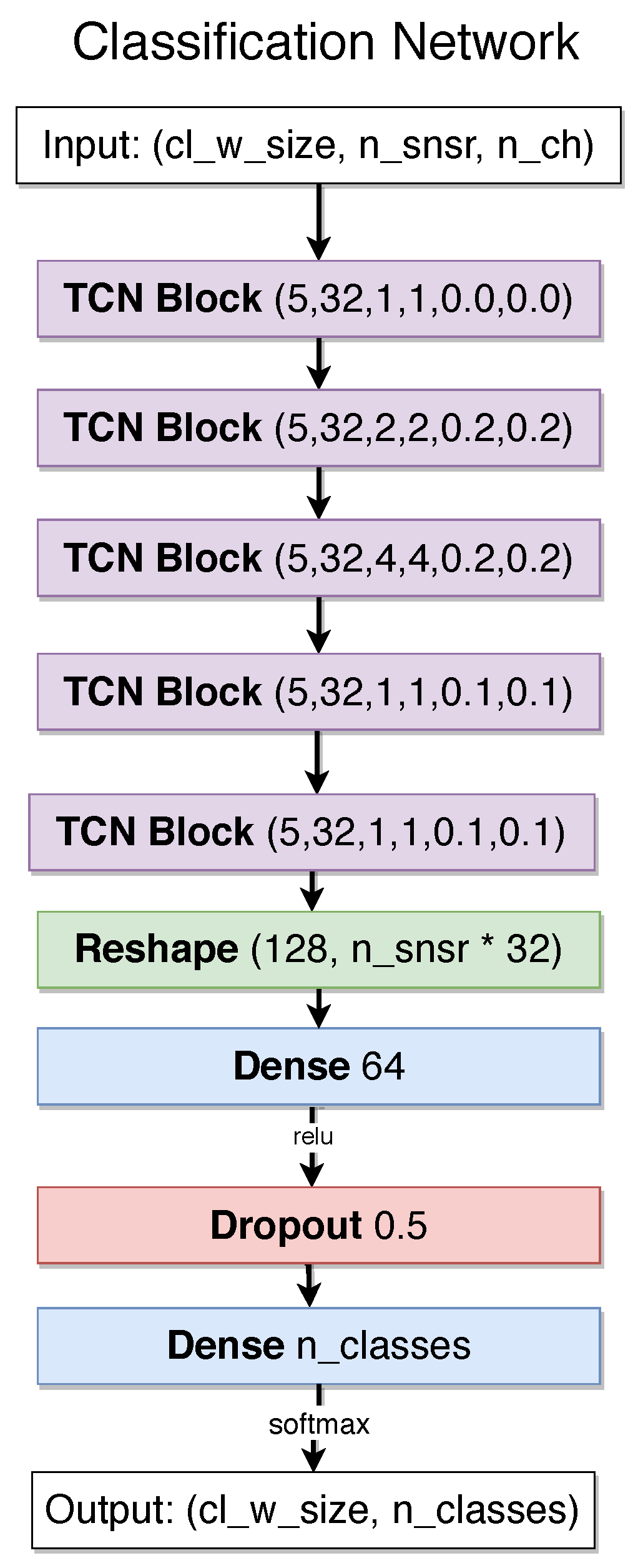
4.3. Recognition Approach

Since the aim of this work is not to optimize the recognition of a specific set of activities but to evaluate the usefulness of simulated sensor data generated from video for wearable HAR systems in general, we use a standard architecture that has proven to be well suited for a variety of activity recognition tasks. The full network architecture can be seen in Figure 8, and, just like the regression model, is based on [42]. The input to the recognition system is $2.56$ s (128 frames) long windows. This window size is sufficient to capture the motions of each exercise, which is repeated many times in a span of 30 s. Since all convolutions in this architecture use same padding, the output class predictions are on frame, not on window level. This allows the network to predict with finer granularity and better deal with cases where two activities are happening inside the same window (transition between activities). For the final prediction we apply majority voting to each window. We trained the network using the categorical cross-entropy loss function and the Adam optimizer [44] with $0.001$ learning rate and $0.9$ and $0.999$ for ${\beta }_1$ and ${\beta }_2$, respectively. Each model is trained for 500 epochs with early stopping using a patience of 25 to avoid overfitting. If any real (not simulated) sensor data is included in a test, a stratified $10\%$ random selection of it is used as the validation set. If no real data is included, the validation set consists of the same selection strategy but applied to all the simulated data. This guarantees the quality of the validation set, while avoiding unfair advantage to configurations that combine simulated and real data. If we simply selected a stratified $10\%$ of all data for validation, tests that combine data (simulated and real) could benefit from having more real points in the training set.

5. Results

5.1. Signal Level Evaluation

Since the aim of our work is not to generate signals that mimic real sensor ones as exactly as possible, but to facilitate training of activity recognition systems that will later be applied to real signals, the key performance indicator is not some sort of numerical dissimilarity measure but the ability to replicate relevant, characteristic signal features that can be used for class discrimination. As the latter is difficult to quantify on signal level, we focus on the quantitative evaluation on the classification tasks with the results being presented in Section 5.3 and Section 5.2.2. Nonetheless it is informative to have a qualitative look at the signals that our system generates for various sensors and how they compare to the real sensor signals generated in the same situation. To this end we consider situations where we have video and sensor data for the same activity. We then plot over each other the actual sensor signal (red in all figures) and the corresponding simulated sensor signal generated by our system (blue in all figures). We begin by looking at signals generated for the dataset that we used for training the regression. This is in a way the easiest task as we do not have to deal with the question of how representative the training dataset that we assembled for our regression model is. In Figure 7 we first consider examples of signals for the accelerometer and gyroscope norm $\sqrt{x^2+y^2+z^2}$. This avoids problems associated with the difficulty of estimating small rotations around the limb axis which have influence in particular on the projection of the gravity vector onto the individual sensor axis. The signals are shown for a period of time of around 10min. For each signal we show the unprocessed signal and a version filtered with 8 Hz (the impact of the filtering will be discussed later). General observations from Figure 7 are:

• Overall the simulated signal has the same trends and large scale features as the original signal.
• Many of the smaller features such as distinct peaks are also matched by the simulated signal. However, some are missed or have a much smaller amplitude in the simulated signal.
• The main difference between the simulated and the real signal is in the amplitude. In most cases the simulated amplitude is smaller, but not by a constant factor that could be overcome with simple scaling. The underestimation is particularly pronounced for high frequency peaks. This can be explained by a number of factors. First of all high frequency components (“details”) tend to be in general more difficult to reproduce and given the limited size of our training set, some limitations in this area are not surprising. Second, in particular for the acceleration sensors, some of the peaks are due to physical effects which are not present or very difficult to capture in the video (e.g., high frequency “ringing” after sudden impact, see Section 2).
• Especially in the acceleration signals there is a “baseline shift”-like effect (especially visible in the third row of Figure 7). At times the system seems to completely ignore parts that are below a baseline situated just below 10 (corresponding to around 1 g). This can be attributed to downward motions where the earth gravity is subtracted from the acceleration. Thus a free falling object (accelerating downwards with 1 g) experiences no acceleration force (is weightless). This means that the acceleration norm is smaller than 1 g (actually 0 in free fall), at least as experienced by the real sensor. For all other motions on the other hand, the value of the acceleration is always equal to or above, at least in the norm, 1 g. Given the limited size of the training set for the regression model and the fact that we did not include any semantic analysis to detect the “down” direction it is not surprising that our model struggles to capture this phenomenon. One way of dealing with the problem is to use linear acceleration which can be derived by IMUs, which is discussed below.

To get a better understanding how the system handles detailed signal features Figure 9 and Figure 10 show zoomed views of 2 signal segments that were selected to cover the “good” as well as the “bad” cases. Figure 9 shows for each signal a comparison of the acceleration and gyro norms. To explore in more detail the issue raised in point 4 above Figure 10 shows not just the acceleration norm, but also the norm of the linear acceleration which excludes the gravity contribution. The main observations are:

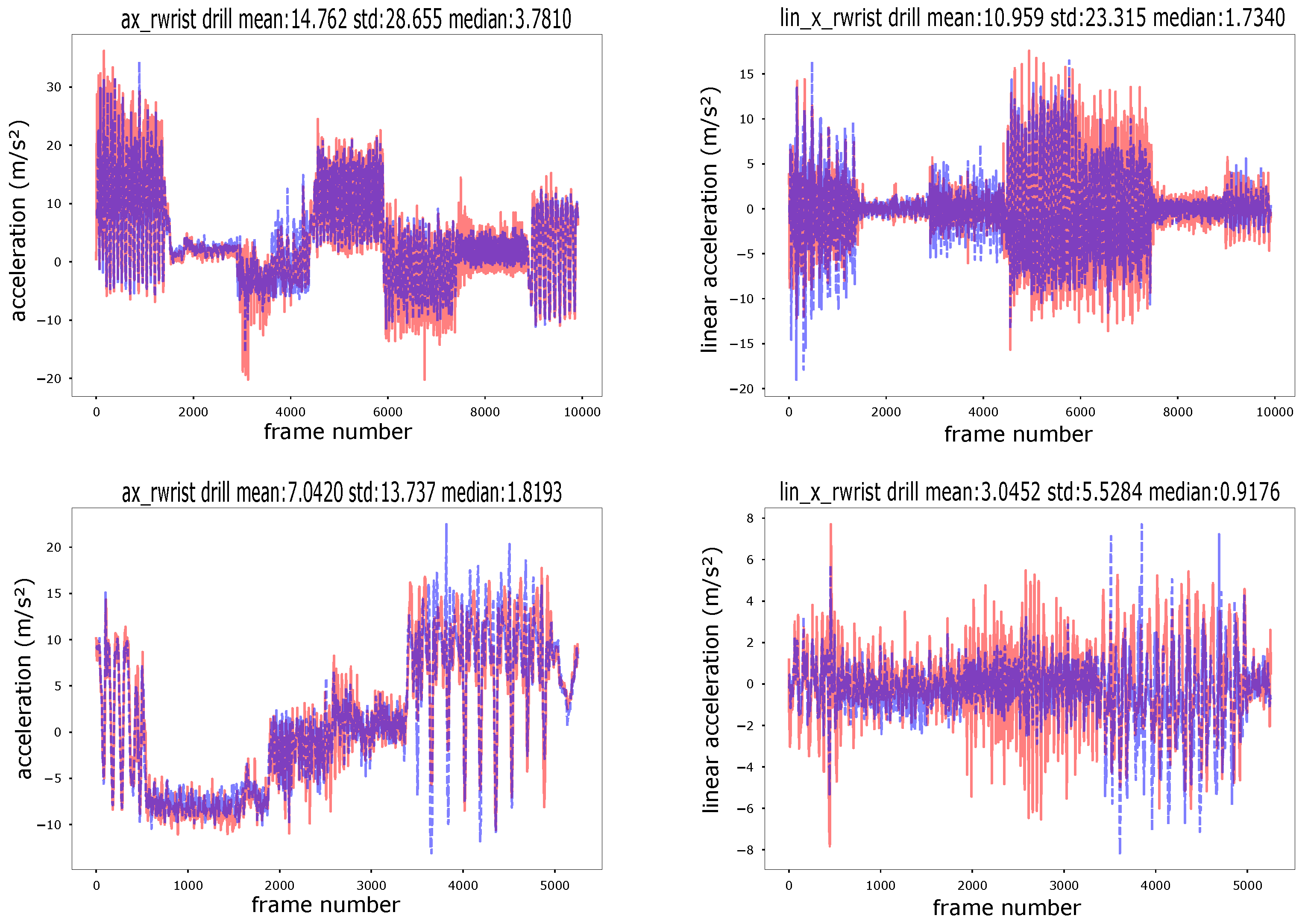
• The left part of Figure 9 shows an example of a “good” simulation. It can be seen that the simulated gyro signal nearly perfectly tracks the real gyro, even through fairly subtle features. Except for the amplitude issues the same holds for the accelerometer signal. Note that while the signal segment contains subtle and fast components, it does not have very high frequency “singular” peaks, which is a key reason why the system works so well here.
• On the right side of Figure 9 a case of much poorer performance is shown. This is largely due to the presence of many singular high frequency, high amplitude peaks which especially the acceleration signal fails to track correctly.
• With respect to the linear acceleration Figure 9 shows two things. First we see on the right side that using the norm linear acceleration instead of the norm raw acceleration signal indeed does solve the problem of the system refusing to model signal values below the baseline of 1 g. On the other hand, as shown in the left part of the figure, using linear acceleration may lead to signal characteristics changing and acquiring additional high frequency peaks which can be difficult to model.

To probe further we have plotted signals from individual acceleration axes as both raw acceleration and linear acceleration in Figure 11 including a zoomed in version in Figure 12. The single axis acceleration signal is richer in features than both the linear acceleration on the same axis and the norm signals discussed above. This in itself is well known and not surprising. What is surprising is how well the simulated signals replicate the real ones given the issues described in Section 2 (e.g., the difficulty of estimating the projection of gravity into individual axis). This applies to both the overall, broad structure of the signal (Figure 11) and, in many cases to the detailed structure. An example is illustrated in Figure 12 on the left where some very subtle features have been matched nearly perfectly. Clearly, other examples exist, as shown on the right of the Figure where there is much more difference between the features of the simulated and the real signal.

5.2. Effects of Pre-Processing

From the above discussion it is apparent that the two main concerns are modelling high frequency components such as acceleration “ringing” caused by sudden forceful impacts and exact matching of the signal magnitude. This suggests the use of low pass filtering and scaling as obvious pre-processing approaches. Both are parts of our pipeline (Section 3.1). Note that we are talking about standard scaling when learning the regression; that is, with the mean and standard deviation computed on our dataset of generic motions being performed by other users. As the mean may be different in this dataset, we simply undo the standard scaling, which is fully reversible, when obtaining simulated signals.

Other pre-processing parameters within our pipeline are the sliding window sizes for training the regression. We experimented with window sizes of 50 and 16 values, representing 1 s and $0.32$ s, respectively. In our early experiments training the regression models, it became clear that the smaller value was better, providing a smaller regression loss and better overall classification. Thus, for brevity, we report all results with the smaller window size. Regarding window step, we keep it at 1 to increase the amount of training data.

5.2.1. Signal Level Effects of Filtering and Scaling

In Figure 13 we illustrate the effect of frequency filtering and scaling on the performance of our regression model. We consider low pass filtering with 12 Hz and 8 Hz (given the original rate of 50 Hz from the video signals). The low pass filtering itself was done using a butterworth low pass filter of the 6th order and standard scaling was done by removing the mean of the sensor channel in the training set and dividing by its standard deviation. Example comparisons of a signal with no filtering and no scaling on one hand and with 8 Hz filtering and scaling on the other are also shown in Figure 7 (left and right column respectively).

Key observations are:

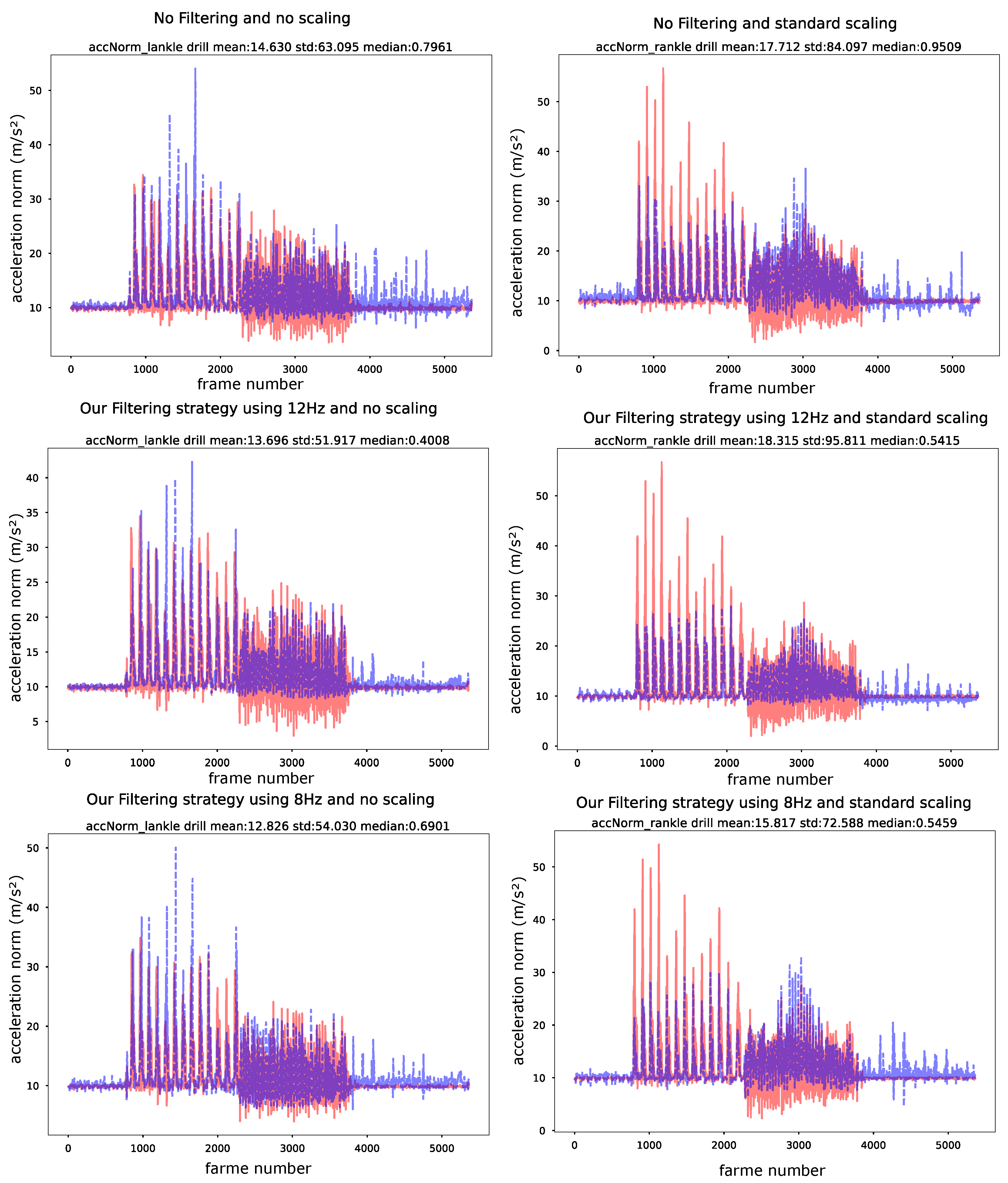
• Overall there is no dramatic effect. In all cases the simulated signal follows the structure of the real signal with reasonable accuracy while displaying the same types of problems.
• Without scaling (left column on Figure 13) there are some pronounced amplitude outliers in the high frequency peaks amplitudes (between sample 1000 and 2000) that are not influenced by the frequency filtering. These disappear in the scaled versions (right column); however, at the cost of significant underestimation of the amplitude in the same area and overestimation around 3000.
• In Figure 13 frequency filtering has little effect, except for reducing the underestimation of the components below 1 g around sample 3000 in the no scaling case (which overall seems to be the best).

In summary while both filtering and scaling do have benefits in some situations, qualitative signal examination does not indicate it to be decisive or obvious. To get a more quantitative idea, Figure 14 shows the Mean Squared Error for computed over all our samples for acceleration and gyroscope for different filter values. For acceleration the error is indeed smaller for 8 Hz (but not by much). For the gyroscope signal there is no significant difference.

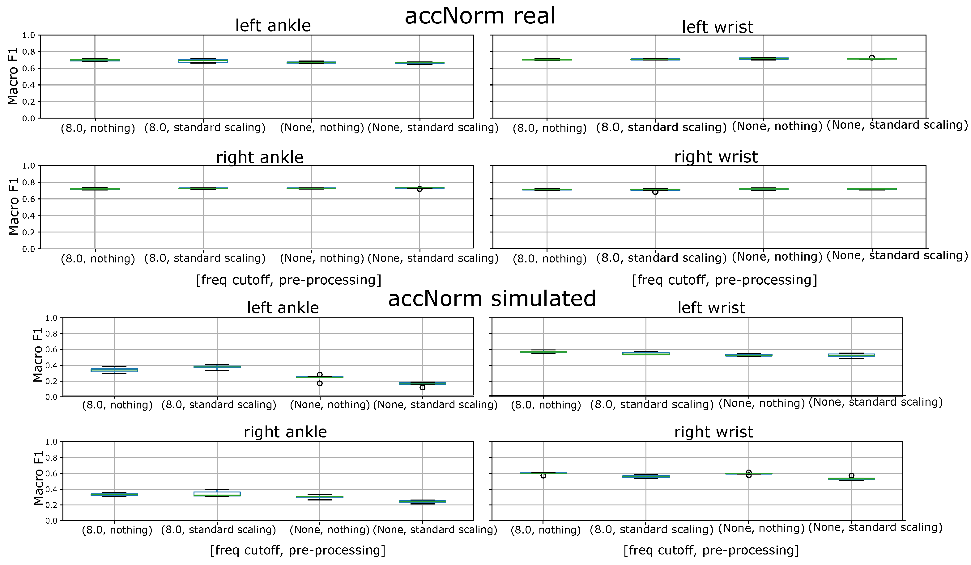
5.2.2. Classification Level Effects of Filtering and Scaling

As a final evaluation step we did an analysis regarding the impact of filtering and scaling on the classification performance. To this end we need to consider not only how the pre-processing impacts the comparison between the classification within simulated sensor data, but also how it impacts the performance of the absolute recognition rates of the real sensor data based models. It makes little sense to apply pre-processing methods that make the results of the simulated signals based model equal to that of a real signals based one but at the cost of making both much worse. In Figure 15 we thus consider the effect of 8 Hz filtering and scaling in different combinations on the recognition for different placements (wrist and ankle) of the sensor for the real and the simulated data. The training was done on all the data designated for training and the testing on all testing data as described in Section 4.2. We can see that the recognition rates on the real data show little sensitivity to the filtering and scaling. The performance on the simulated data is also fairly invariant for the wrist sensor placement while for the ankle placement frequency filtering does indeed make a significant difference. However, it must also be noted that for the ankle placement the recognition rate with the simulated data is very poor to start with (around 40%).

5.3. Evaluation of Classification Performance Using the Simulated Signals

The discussion in the previous section has shown that, mostly on a qualitative level, our method generates signals that replicate a significant portion of the respective real sensor output within our application domain. We now proceed to quantitatively evaluate how well such simulated sensor signals are suited for training activity recognition that will later be applied to real sensor signals. The evaluation procedure has already been described in Section 4.2. Essentially we have recorded a dataset where for each activity and user we have both a video signal and sensor data. In addition, we have collected some YouTube videos for the same/similar activities. We then train classifiers using the real sensor data, simulated sensor data from the videos that we have recorded, simulated sensor data from the YouTube videos and various combinations thereof. The classifier trained on real sensor data is the one to which we compare the performance of the different combinations to evaluate the usefulness of our approach. Given the discussion in the previous section, we focus on using raw data without filtering and scaling with some examples of the impact of 8 Hz filtering. The results are shown in Figure 16, Figure 17 and Figure 18. In each figure, we plot the recognition rate of each classifier vs. the number of users in the training set. The only exception is the case of sensor data generated from YouTube videos where we had different users perform different exercises from the set which means that the notion of “number of users” for the whole dataset makes no sense (see Table 1). Instead, we have generated training data from the entire 14 min of the YouTube data that we harvested and plotted it for comparison as a constant in the graphs.

• Baseline. The recognition rates on the real data reach up to 90% which, given the fact that our aim was not to optimize a recognition system for a specific application, is an acceptable baseline to evaluate the performance of the simulated sensor data.
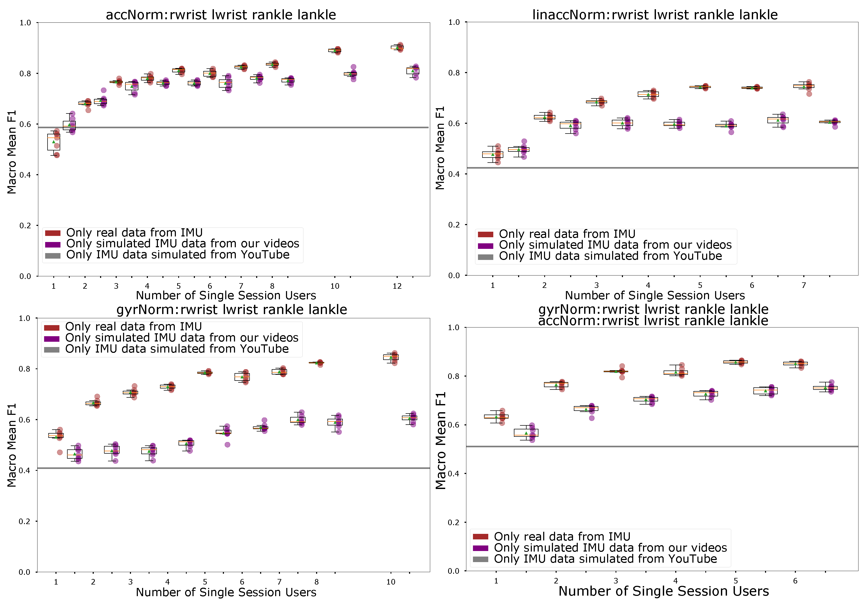
• Overall performance on simulated sensor data. Systems trained on the simulated data reach up to 80% recognition rate, which is 10% below the results (see e.g., Figure 16 left where the acceleration norm based recognition is among the best performing variants overall). In general as the number of users is small the results for real and simulated data are very similar to the performance of the real data. The performance on the real sensor data improves faster with the amount of training data. This is to be expected as with a very small number of users (equal a small amount of training data) the recognition rate tends to be poor and limiting factor for the performance is the lack of diversity in the data and not the data quality. As the amount of data increases, the quality becomes the limiting factor, which is better for the real sensor data.
• Performance on YouTube data. The performance of the system based on sensor data simulated from YouTube videos is in most cases slightly below the performance of the baseline on a single or two users. Given that the total amount of YouTube data (around 14 min) is in the order of magnitude of the length of the data from a single user this is not surprising.
• Compensating deficiencies of simulated data through training set size. There is strong indication that deficiencies of the simulated sensor data can be compensated by the amount of such data. Thus in most cases (see discussion of different sensor combinations later on) systems based on simulated sensor data can match the performance of the real sensor data based system trained on about half as much data. Again looking at the acceleration norm from all sensors case in Figure 16 left top we see that the Mean F1 score for simulated data with 12 users is about the same as the score for 6 users with real data. Furthermore, while we see a slower growth of the F1 score with the number of users in the training set for the case of simulated data than for real data, in most cases growth exists.
• Effects of model fine tuning using real sensor data. Another way to improve the performance of the simulated sensor data based systems is to use small amounts of real sensor data to fine-tune it. The idea is that collecting a small amount of real data is nearly always possible, it is the bulk of a large training data set that is difficult to collect and that we want to get from existing videos. The results of this strategy are illustrated in Figure 17. We compare the baseline to the performance of a system trained on simulated data to which 1 (blue points) or 2 (yellow points) users with real data have been added. We can see that the simulated data is now much closer to the real one. In the top left graph showing the acceleration norm results it is virtually identical up to 10 users when the real data starts to overtake the simulated one. The effect is even more significant for the gyro norm based recognition (see Figure 17 right top) where the purely simulated signals based model trailed the real signals based ones by 30% and more (see Figure 16 left bottom) and are now not worse than about 10% worse (and up to 6 users nearly identical).
• Effects of adding simulated data from YouTube to small amounts of real data. Another situation where a combination of real and simulated signals may be useful is when we have only a small amount of sensor-based training data with no easy possibility of collecting more. We then try to “top up” our training set with some simulated data from video. The effect of such a strategy is illustrated by the green points (real IMU data with YouTube) in Figure 17 where we combine the real sensor data with the YouTube data increasing the number of real data over the x axis. We can see that for small user numbers the strategy indeed helps.
• Performance of different sensors and sensor combinations. Most of the discussion so far has been done with respect to the acceleration norm (Figure 16 and Figure 17) applied to both wrists and both ankles together which has been the most effective modality with respect to the recognition performance both in the real sensor signal and with respect to how well the simulated signal can approximate it. Given the type of activities that we use as our test set this is not surprising. The activities are characterized by periodic, mostly strong motions of various limbs. In most cases the relative temporal pattern and relative intensity of the motions is a characteristic feature. At the same time, the acceleration norm (in particular when looking at the relative intensity and temporal patterns) is fairly robust against variations and noise. This also means that imperfections caused by the simulation of the signal from the video data using our regression model can be well tolerated.
  Further sensor modalities and their combinations that we investigated are:

  (a)

  Acceleration norm vs. Gyro norm vs. combination. In Figure 16 we have in addition to the acceleration norm the linear acceleration norm, the gyroscope norm, and the combination of gyroscope and acceleration norms (in all cases for all the 4 sensor placements). The first thing we see is that the linear acceleration leads to a poorer overall performance while having little impact on the relative performance of the simulated data. The former is not surprising since the gravity component (meaning vertical orientation) is a very important piece of information. The latter is contrary to what we might have expected since our model was not tuned to capture gravity effects (as discussed in Section 2). Apparently it was still able to capture a sufficient amount of orientation related information. Second, we see that the gyro signal has significantly worse relative performance for the simulated signal. Given the limitations on recognizing rotations around certain axes (in particular the limb axis) from the video signal discussed in Section 2 this was to be expected. The very poor performance of the simulated gyro signal also drags down the combined acceleration/gyro norm performance shown in the bottom right part of Figure 16.

  (b)

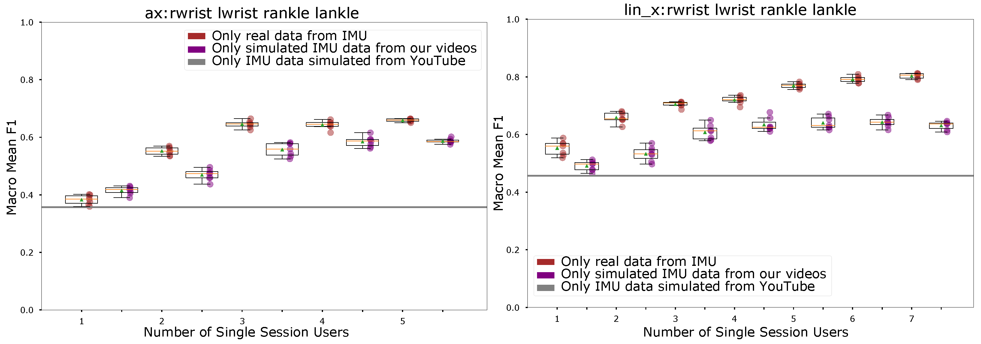
  Acceleration and linear acceleration on the limb’s axis. Further looking at the impact of linear acceleration Figure 18 shows the results for raw acceleration and linear acceleration along the limb axis. The idea is that the acceleration along the axis is independent of the rotation around the axis, which, as already explained is hard to exactly capture from video. It can be seen that both have slightly lower performance than the acceleration norm (which is not surprising given that the acceleration norm is a good discriminator for our set of activities as described above). Within expected statistical bounds the difference between the simulated and the real sensor signal is about the same for both the raw and the linear acceleration.

  (c)

  Different sensor placements. In Section 5.2.2 we have already considered the use of sensors from only a wrist or only the ankle (with respect to acceleration norm) as shown in Figure 15. The performance for the real sensor data on both the wrist and the ankle and the simulated sensor data on the wrist was with around 10–20% less than for the combination which is not a surprising result (both legs and arms are relevant for our test activities). What may be surprising at first is the fact that the performance for the ankle using simulated data is half that of the real data (30–40%). The explanation is that foot motions involve a lot of hard ground impacts that lead to “ringing” that has already often been mentioned as something that the simulated data cannot replicate (which is why 8 Hz filtering helps a lot here). In addition vertical orientation plays a bigger role than for the wrists and there are many motions “to the front” (towards the camera) which are more difficult to resolve due to the viewing angle.

• Effects of 8 Hz Filtering. The effect of various pre-processing strategies has already been discussed in Section 5.2 establishing that while filtering and to some degree scaling did seem to be beneficial in some cases, overall the effect was not overwhelming given that these effects may be strongly application specific. This is why we have decided to do most of the analysis in this section on the unfiltered, not scaled signal. However, for comparison Figure 19 includes the same evaluation done in Figure 16 with 8 Hz filtering. We can see that, while for the gyro norm (which was the poorest one to start with) the filtering does indeed improve the relative performance of the simulated signal based model, it has little effect otherwise.

6. Conclusions and Future Work

The main result of our work is the demonstration of the basic feasibility of using deep network regression models to generate simulated IMU signals directly from video extracted postures. This includes the detailed analysis of the influence of different design decisions on the performance and also includes discussion of the problems that need to be addressed to improve the results. In the long term, this work should contribute to the creation of training datasets that are comparable in size to what exists in computer vision today and thus facilitate a more profound impact of deep learning techniques on wearable sensors based HAR.

Clearly the work described here is just a first step towards this vision. Based on the results described and discussed in the previous section we consider the following to be the most promising next steps that we will investigate:

Extending the training data set for our regression model, in terms of the number of users, the variety of motions and the number of sensor placements. This includes also handling different camera positions and more complex poses. For example, lying on a mat or swimming.

Collecting a large set of online videos for a more diverse set of activities, and further testing and fine-tuning our model on them.

Extending the regression model to handle all types of sensor signals (e.g., acceleration and gyro on each axis) better. This includes considering relations between sensor signals e.g., the orientation of the wrist IMU in the frame of reference of the hip or back mounted IMU which is often used as relevant information in wearable activity recognition systems.

Implicit modeling of gravity by exploring image segmentation based detection of “down” direction and including the angle towards the down vector in the features that we feed our regression model. This will be particularly important as we start looking at more and more complex sensor signals as mentioned above.

Exploring training the regression using the concept of Physically Informed Networks [45] that incorporate physical constraints as regularization terms. The idea is to build a regression model that for example simultaneously trains the ax, ay and az component of the acceleration and the corresponding norm $\left|a\right|$ and embedding the $\left|a\right|=\sqrt{a{x}^2+a{y}^2+a{z}^2}$ in the regularization term. Relationships between the accelerometer and the gyroscope sensor signal at the same location and temporal conditions could also be considered. These are all especially relevant for generating more complex sensor signals as described in the previous points.

(6)

We could also explore applying our method to (more) easily identifiable locations where sensors should be placed on the body for a specific set of activities. Before recording sensor data, videos of those activities can be collected and sensor values simulated for different on-body locations, which then can help select the best locations to place them when recording training data.

References

1. Lara, O.D.; Labrador, M.A. A survey on human activity recognition using wearable sensors. IEEE Commun. Surv. Tutor. 2012, 15, 1192–1209. [Google Scholar] [CrossRef]
2. Wang, J.; Chen, Y.; Hao, S.; Peng, X.; Hu, L. Deep learning for sensor-based activity recognition: A survey. Pattern Recognit. Lett. 2019, 119, 3–11. [Google Scholar] [CrossRef] [Green Version]
3. Sun, C.; Shrivastava, A.; Singh, S.; Gupta, A. Revisiting unreasonable effectiveness of data in deep learning era. In Proceedings of the IEEE International Conference on Computer Vision, Venice, Italy, 22–29 October 2017; pp. 843–852. [Google Scholar]
4. Brain, D.; Webb, G. On the effect of data set size on bias and variance in classification learning. In Proceedings of the Fourth Australian Knowledge Acquisition Workshop; University of New South Wales: Sydney, Australia, 1999; pp. 117–128. [Google Scholar]
5. Wang, L.; Gjoreski, H.; Ciliberto, M.; Lago, P.; Murao, K.; Okita, T.; Roggen, D. Summary of the Sussex-Huawei Locomotion-Transportation Recognition Challenge 2020. In Adjunct Proceedings of the 2020 ACM International Joint Conference on Pervasive and Ubiquitous Computing and Proceedings of the 2020 ACM International Symposium on Wearable Computers; Association for Computing Machinery: New York, NY, USA, 2020; pp. 351–358. [Google Scholar] [CrossRef]
6. Russakovsky, O.; Deng, J.; Su, H.; Krause, J.; Satheesh, S.; Ma, S.; Huang, Z.; Karpathy, A.; Khosla, A.; Bernstein, M.; et al. ImageNet Large Scale Visual Recognition Challenge. Int. J. Comput. Vis. (IJCV) 2015, 115, 211–252. [Google Scholar] [CrossRef] [Green Version]
7. Knoll, F.; Murrell, T.; Sriram, A.; Yakubova, N.; Zbontar, J.; Rabbat, M.; Defazio, A.; Muckley, M.J.; Sodickson, D.K.; Zitnick, C.L.; et al. Advancing machine learning for MR image reconstruction with an open competition: Overview of the 2019 fastMRI challenge. Magn. Reson. Med. 2020, 84, 3054–3070. [Google Scholar] [CrossRef] [PubMed]
8. Reiss, A.; Stricker, D. Creating and benchmarking a new dataset for physical activity monitoring. In Proceedings of the 5th International Conference on PErvasive Technologies Related to Assistive Environments, Crete, Greece, 6–8 June 2012; pp. 1–8. [Google Scholar]
9. Reiss, A.; Stricker, D. Introducing a new benchmarked dataset for activity monitoring. In Proceedings of the 2012 16th International Symposium on Wearable Computers, Newcastle, UK, 18–22 June 2012; pp. 108–109. [Google Scholar]
10. Chavarriaga, R.; Sagha, H.; Calatroni, A.; Digumarti, S.T.; Tröster, G.; Millán, J.d.R.; Roggen, D. The Opportunity challenge: A benchmark database for on-body sensor-based activity recognition. Pattern Recognit. Lett. 2013, 34, 2033–2042. [Google Scholar] [CrossRef] [Green Version]
11. Roggen, D.; Calatroni, A.; Rossi, M.; Holleczek, T.; Förster, K.; Tröster, G.; Lukowicz, P.; Bannach, D.; Pirkl, G.; Ferscha, A.; et al. Collecting complex activity datasets in highly rich networked sensor environments. In Proceedings of the 2010 Seventh International Conference on Networked Sensing Systems (INSS), Kassel, Germany, 15–18 June 2010; pp. 233–240. [Google Scholar]
12. Deng, J.; Dong, W.; Socher, R.; Li, L.J.; Li, K.; Fei-Fei, L. Imagenet: A large-scale hierarchical image database. In Proceedings of the 2009 IEEE Conference on Computer Vision and Pattern Recognition, Miami, FL, USA, 20–25 June 2009; pp. 248–255. [Google Scholar]
13. Smaira, L.; Carreira, J.; Noland, E.; Clancy, E.; Wu, A.; Zisserman, A. A Short Note on the Kinetics-700-2020 Human Action Dataset. arXiv 2020, arXiv:cs.CV/2010.10864. [Google Scholar]
14. Rey, V.F.; Hevesi, P.; Kovalenko, O.; Lukowicz, P. Let There Be IMU Data: Generating Training Data for Wearable, Motion Sensor Based Activity Recognition from Monocular RGB Videos. In Adjunct Proceedings of the 2019 ACM International Joint Conference on Pervasive and Ubiquitous Computing and Proceedings of the 2019 ACM International Symposium on Wearable Computers; Association for Computing Machinery: New York, NY, USA, 2019; pp. 699–708. [Google Scholar] [CrossRef]
15. Asare, P.; Dickerson, R.F.; Wu, X.; Lach, J.; Stankovic, J.A. BodySim: A multi-domain modeling and simulation framework for body sensor networks research and design. In Proceedings of the 11th ACM Conference on Embedded Networked Sensor Systems, Roma, Italy, 5–11 November 2013; pp. 1–2. [Google Scholar]
16. Ascher, C.; Kessler, C.; Maier, A.; Crocoll, P.; Trommer, G. New pedestrian trajectory simulator to study innovative yaw angle constraints. In Proceedings of the 23rd International Technical Meeting of The Satellite Division of the Institute of Navigation (ION GNSS 2010), 21–24 September 2010; pp. 504–510. [Google Scholar]
17. Young, A.D.; Ling, M.J.; Arvind, D.K. IMUSim: A simulation environment for inertial sensing algorithm design and evaluation. In Proceedings of the 10th ACM/IEEE International Conference on Information Processing in Sensor Networks, Chicago, IL, USA, 12–14 April 2011; pp. 199–210. [Google Scholar]
18. Zampella, F.J.; Jiménez, A.R.; Seco, F.; Prieto, J.C.; Guevara, J.I. Simulation of foot-mounted IMU signals for the evaluation of PDR algorithms. In Proceedings of the 2011 International Conference on Indoor Positioning and Indoor Navigation, Portland, OR, USA, 21–24 September 2011; pp. 1–7. [Google Scholar]
19. Smith, M.; Moore, T.; Hill, C.; Noakes, C.; Hide, C. Simulation of GNSS/IMU measurements. In Proceedings of the ISPRS International Workshop. Working Group I/5: Theory, Technology and Realities of Inertial/GPS Sensor Orientation, Castelldefels, Spain, 22–23 September 2003; pp. 22–23. [Google Scholar]
20. Parés, M.; Rosales, J.; Colomina, I. Yet another IMU simulator: Validation and applications. In Proceedings of the Eurocow, Castelldefels, Spain, 30 January–1 February 2008. [Google Scholar]
21. Cao, Z.; Hidalgo, G.; Simon, T.; Wei, S.E.; Sheikh, Y. OpenPose: Realtime multi-person 2D pose estimation using Part Affinity Fields. arXiv 2018, arXiv:1812.08008. [Google Scholar] [CrossRef] [PubMed] [Green Version]
22. Banos, O.; Calatroni, A.; Damas, M.; Pomares, H.; Rojas, I.; Sagha, H.; del R. Mill´n, J.; Troster, G.; Chavarriaga, R.; Roggen, D. Kinect=IMU? Learning MIMO Signal Mappings to Automatically Translate Activity Recognition Systems across Sensor Modalities. In Proceedings of the 2012 16th International Symposium on Wearable Computers, Newcastle, UK, 18–22 June 2012; pp. 92–99. [Google Scholar]
23. Kanazawa, A.; Black, M.J.; Jacobs, D.W.; Malik, J. End-to-end recovery of human shape and pose. In Proceedings of the IEEE Conference on Computer Vision and Pattern Recognition, Salt Lake City, UT, USA, 18–22 June 2018; pp. 7122–7131. [Google Scholar]
24. Elhayek, A.; Kovalenko, O.; Murthy, P.; Malik, J.; Stricker, D. Fully Automatic Multi-person Human Motion Capture for VR Applications. In Proceedings of the International Conference on Virtual Reality and Augmented Reality—EuroVR, London, UK, 22–23 October 2018; pp. 28–47. [Google Scholar]
25. Mehta, D.; Sridhar, S.; Sotnychenko, O.; Rhodin, H.; Shafiei, M.; Seidel, H.P.; Xu, W.; Casas, D.; Theobalt, C. Vnect: Real-time 3D human pose estimation with a single rgb camera. ACM Trans. Gr. 2017, 36, 44. [Google Scholar] [CrossRef] [Green Version]
26. Rogez, G.; Weinzaepfel, P.; Schmid, C. Lcr-net++: Multi-person 2d and 3d pose detection in natural images. IEEE Trans. Pattern Anal. Mach. Intell. 2019, 42, 1146–1161. [Google Scholar] [CrossRef] [PubMed] [Green Version]
27. Murthy, P.; Kovalenko, O.; Elhayek, A.; Gava, C.C.; Stricker, D. 3D Human Pose Tracking inside Car using Single RGB Spherical Camera. In Proceedings of the ACM Chapters Computer Science in Cars Symposium (CSCS); ACM: New York, NY, USA, 2017. [Google Scholar]
28. Omran, M.; Lassner, C.; Pons-Moll, G.; Gehler, P.; Schiele, B. Neural body fitting: Unifying deep learning and model based human pose and shape estimation. In Proceedings of the 2018 international conference on 3D vision (3DV), Verona, Italy, 5–8 September 2018; pp. 484–494. [Google Scholar]
29. Bogo, F.; Kanazawa, A.; Lassner, C.; Gehler, P.; Romero, J.; Black, M.J. Keep it SMPL: Automatic estimation of 3D human pose and shape from a single image. In European Conference on Computer Vision; Springer: Berlin/Heidelberg, Germany, 2016; pp. 561–578. [Google Scholar]
30. Yao, S.; Zhao, Y.; Shao, H.; Zhang, C.; Zhang, A.; Hu, S.; Liu, D.; Liu, S.; Su, L.; Abdelzaher, T. Sensegan: Enabling deep learning for internet of things with a semi-supervised framework. Proc. ACM Interact. Mob. Wearable Ubiquitous Technol. 2018, 2, 144. [Google Scholar] [CrossRef] [Green Version]
31. Li, X.; Luo, J.; Younes, R. ActivityGAN: Generative adversarial networks for data augmentation in sensor-based human activity recognition. In Proceedings of the Adjunct Proceedings of the 2020 ACM International Joint Conference on Pervasive and Ubiquitous Computing and Proceedings of the 2020 ACM International Symposium on Wearable Computers; ACM: New York, NY, USA, 2020; pp. 249–254. [Google Scholar]
32. Radhakrishnan, S. Domain Adaptation of IMU Sensors Using Generative Adversarial Networks. 2020. Available online: https://www.diva-portal.org/smash/record.jsf?pid=diva2%3A1505604&dswid=5801 (accessed on 1 January 2021).
33. Qian, X.; Fu, Y.; Xiang, T.; Wang, W.; Qiu, J.; Wu, Y.; Jiang, Y.G.; Xue, X. Pose-normalized image generation for person re-identification. In Proceedings of the European conference on computer vision (ECCV), Munich, Germany, 8–14 September 2018; pp. 650–667. [Google Scholar]
34. Sirignano, J.; Spiliopoulos, K. DGM: A deep learning algorithm for solving partial differential equations. J. Comput. Phys. 2018, 375, 1339–1364. [Google Scholar] [CrossRef] [Green Version]
35. Raissi, M.; Perdikaris, P.; Karniadakis, G.E. Physics informed deep learning (part i): Data-driven solutions of nonlinear partial differential equations. arXiv 2017, arXiv:1711.10561. [Google Scholar]
36. Takeda, S.; Okita, T.; Lago, P.; Inoue, S. A Multi-Sensor Setting Activity Recognition Simulation Tool. In Proceedings of the 2018 ACM International Joint Conference and 2018 International Symposium on Pervasive and Ubiquitous Computing and Wearable Computers; ACM: New York, NY, USA, 2018; pp. 1444–1448. [Google Scholar] [CrossRef]
37. Lago, P.; Takeda, S.; Okita, T.; Inoue, S. MEASURed: Evaluating Sensor-Based Activity Recognition Scenarios by Simulating Accelerometer Measures from Motion Capture. In Human Activity Sensing; Springer: Berlin, Germany, 2019; pp. 135–149. [Google Scholar]
38. Kwon, H.; Tong, C.; Haresamudram, H.; Gao, Y.; Abowd, G.D.; Lane, N.D.; Ploetz, T. IMUTube: Automatic extraction of virtual on-body accelerometry from video for human activity recognition. arXiv 2020, arXiv:2006.05675. [Google Scholar] [CrossRef]
39. Radu, V.; Henne, M. Vision2Sensor: Knowledge Transfer Across Sensing Modalities for Human Activity Recognition. Proc. ACM Interact. Mob. Wearable Ubiquitous Technol. 2019, 3. [Google Scholar] [CrossRef] [Green Version]
40. Video that was Followed to Produce the Drill Dataset. Available online: https://www.youtube.com/watch?v=R0mMyV5OtcM (accessed on 6 July 2020).
41. Cao, Z.; Simon, T.; Wei, S.E.; Sheikh, Y. Realtime multi-person 2d pose estimation using part affinity fields. In Proceedings of the IEEE Conference on Computer Vision and Pattern Recognition, Honolulu, HI, USA, 21–26 July 2017; pp. 7291–7299. [Google Scholar]
42. Bai, S.; Kolter, J.Z.; Koltun, V. An empirical evaluation of generic convolutional and recurrent networks for sequence modeling. arXiv 2018, arXiv:1803.01271. [Google Scholar]
43. He, K.; Zhang, X.; Ren, S.; Sun, J. Deep residual learning for image recognition. In Proceedings of the IEEE Conference on Computer Vision and Pattern Recognition, Las Vegas, NV, USA, 27–30 June 2016; pp. 770–778. [Google Scholar]
44. Kingma, D.P.; Ba, J. Adam: A Method for Stochastic Optimization. arXiv 2014, arXiv:1412.6980. [Google Scholar]
45. Raissi, M.; Perdikaris, P.; Karniadakis, G.E. Physics-informed neural networks: A deep learning framework for solving forward and inverse problems involving nonlinear partial differential equations. J. Comput. Phys. 2019, 378, 686–707. [Google Scholar] [CrossRef]
46. Video that was Followed to Produce our Seed Motions. Available online: https://www.youtube.com/watch?v=14Cyw7VDsw0 (accessed on 24 March 2021).
Figure 1. The steps involved in applying our overall method. In step 1 we record video and sensor data for a broad set of generic motions typical for a given domain. Using this data we train models to map the videos onto the corresponding sensor data. Step 2 consists of acquiring for each new recognition task a set of labeled videos of the respective activities from online repositories. The videos are then fed to the regression models which generate their simulated sensor data. Since the labels for the sensor data are identical to the video labels, we now have labeled training sensor data, which we use to train a recognition model for the required activities (step 3). The final step is 4, where we use the trained model to recognize those activities from real sensor data in the end application.
Applsci 11 03094 g001
Figure 2. Short depiction of the motions present in the 10 exercises of the Drill dataset, in which participants performed the exercises of [40]. The first examples are of one of our subjects, while the last are from the original YouTube video each subject tries to replicate. In this dataset, each exercise is repeated once for 30 s.
Applsci 11 03094 g002
Figure 3. Joints used for each of the 4 regression models. Those models also receive the scaled hip speed and the change in scale. Orange boxes represent where sensors were placed during the exercises, while their surrounding white boxes describe the joints relevant for each of their regression models.
Applsci 11 03094 g003
Figure 4. Procedure for training our regression models, which translates sequences of poses to the sensor values they generate. Using a dataset that includes both video and sensor data, we train for each position and sensor channel a regression model that uses the relevant joints and other features to predict the sensor values for that channel and place.
Applsci 11 03094 g004
Figure 5. Architecture for the neural network used for regression of a single sensor.
Applsci 11 03094 g005
Figure 6. Example of a subject performing some of the movements present in our generic motions dataset used for training the regression model. The video followed can be found in [46].
Applsci 11 03094 g006
Figure 7. Real signals (red) versus simulated (blue) in the regression training set (generic motions) for the norm of signals.
Applsci 11 03094 g007
Figure 8. Architecture for the neural network used for classification. For a definition of the blocks see Figure 5. The size of the window for classification was 128, representing 2.56 s and the number of classes in our target dataset is 10.
Applsci 11 03094 g008
Figure 9. Real signals (red) versus simulated (blue) in the regression training set (generic motions) for acceleration and gyro norm. All cases trained without neither filtering nor standard scaling.
Applsci 11 03094 g009
Figure 10. Real signals (red) versus simulated (blue) in the regression training set (generic motions) for acceleration norm, linear and not. All cases trained without neither filtering nor standard scaling.
Applsci 11 03094 g010
Figure 11. Examples of the signals generated by our system in the target dataset (fitness exercises). Specifically we show the acceleration parallel to the lower arm (left) and the linear acceleration along the same axis (acceleration without the gravity component that Inertial Measurement Units (IMUs) can derive with the help of gyro and magnetic field sensors).
Applsci 11 03094 g011
Figure 12. Real signals (red) versus simulated (blue) in the regression training set (generic motions) for acceleration and linear acceleration both in the limb’s axis. All cases trained without neither filtering nor standard scaling.
Applsci 11 03094 g012
Figure 13. Examples signals generated by our method (blue) and their real counterparts (red) in the target dataset (fitness exercises) under different filter and scaling strategies.
Applsci 11 03094 g013
Figure 14. Loss for all windows using different training strategies for acceleration (left) and gyroscope norm (right).
Applsci 11 03094 g014
Figure 15. Comparison of classification performance for models trained with real (upper) or simulated data (down) under different preprocessing techniques using the acceleration norm. Results are shown for each different sensor placement separately.
Applsci 11 03094 g015
Figure 16. Results when using the accelerometer and gyro norm and the combination thereof.
Applsci 11 03094 g016
Figure 17. Results when using the gyroscope and accelerometer norms and adding simulated data to the real one.
Applsci 11 03094 g017
Figure 18. Results when using the linear acceleration in the limb axis.
Applsci 11 03094 g018
Figure 19. Results when using the gyroscope and accelerometer norms and also 8 Hz filtering.
Applsci 11 03094 g019