Numerical and One-Dimensional Studies of Supersonic Ejectors for Refrigeration Application: The Significance of Wall Pressure Variation in the Converging Mixing Section

Abstract

This paper studies the pressure variation that exists on the converging mixing section wall of a supersonic ejector for refrigeration application. The objective is to show that the ejector one-dimensional model can be improved by considering this wall’s pressure variation which is typically assumed constant. Computational Fluid Dynamics (CFD) simulations were used to obtain the pressure variation on the aforementioned wall. Four different ejectors were simulated. An ejector was obtained from a published experimental work and used to validate the CFD simulations. The other three ejectors were a modification of the first ejector and used for the parametric study. The secondary mass flow rate, ${\dot{m}}_s$, was the main parameter to compare. The CFD validation results indicate that the transition SST turbulence model is better than the k-omega SST model in predicting the ${\dot{m}}_s$. The results of the ejector one-dimensional model were compared before and after incorporating the wall pressure variation. The comparison shows that the effect of the pressure variation is significant at certain operating conditions. Even around 2% change in the average pressure can give around 32% difference in the prediction of ${\dot{m}}_s$. For the least sensitive case, around 2% change in the average pressure can give around 7% difference in the prediction.

1. Introduction

Energy-saving topic gains more attention globally. This is a logical consequence of the increase in people’s awareness all over the world regarding the limited fossil energy resources. It keeps depleting and eventually will become extinct. To solve this issue, many researchers have been searching for renewable energy resources as well as developing efficient technologies to utilize that energy. These attempts have led researchers to various ideas such as an idea to use ejectors in refrigeration systems to compress the refrigerant. Instead of using electricity, an ejector is able to utilize thermal energy to do the compression.

An ejector is a device that entrains a fluid at low pressure (secondary flow) by accelerating another fluid at high pressure (primary flow) via a nozzle. Then, the primary and secondary flows mix inside the device and leave through an outlet at an intermediate pressure. In an ejector refrigeration system, the secondary flow is the refrigerant leaving the evaporator, and the ejector acts as a compressor through which this refrigerant is compressed. A typical structure of an ejector can be seen in Figure 1. In this work, the mixing section consists of a converging mixing section, also called constant pressure mixing section, and a constant area mixing section, also called ejector throat (ET) (Figure 1).

A supersonic ejector operation can be divided into three modes, i.e., critical (double-choked) mode, sub-critical (single-choked) mode, and malfunction mode [1]. Figure 2 shows various ejector operation modes at a fixed primary and secondary inlet pressures. The ejector is in a critical mode operation when the primary and secondary flows are both choked. This means that both mass flow rates are constant with respect to the change of ejector outlet pressure, $P_4$. The secondary flow is choked because it accelerates until it reaches sonic speed through a hypothetical converging annular duct formed by the outer boundary of the primary flow jet and the wall of the ejector [2].

As we increase the outlet pressure, the secondary flow will not be choked anymore (only the primary flow is choked). This pressure threshold is referred to as critical pressure,$P_{crit}$. Beyond this pressure, the ejector will enter the sub-critical mode operation within which an increase in $P_4$ will decrease the secondary mass flow rate but has no effect on the primary mass flow rate.

As the outlet pressure is increased further, it reaches a pressure, $P_{mal}$, at which the ejector starts to malfunction. There will be no secondary flow or, even, reverse flow through the secondary inlet will occur. In practice, an ejector is usually required to operate in the critical mode/condition, and hence, it is also called the on-design condition.

Designing an ejector is an important task so that the system utilizing this device is not only able to operate functionally, but also efficiently. To know/predict the performance of an ejector, analytical and computational fluid dynamics (CFD) models are usually used before experiment.

The one-dimensional analytical model has an advantage over the CFD for its simplicity and quick result. It does not require the time-consuming generation of the discretized computational domain. Furthermore, the calculation time is also short, in the order of a few minutes or even seconds, compared to that of CFD which can take hours. Due to these advantages, the one-dimensional model is attractive to predict the global performance of an ejector such as predicting the primary and secondary mass flow rates (${\dot{m}}_p$ and ${\dot{m}}_s$) and the ejector outlet pressure ($P_4$). To improve the model’s accuracy, the effects of local flow phenomena have to be included [1]. Such effects can only be analyzed if the detail of the flow is obtained either by experiment or CFD simulation or both.

The works of Keenan and Neumann [3] as well as Keenan et al. [4] have become the basis of many researchers doing ejector one-dimensional modeling. Many attempts have been done to improve the model’s prediction of ejector behavior by considering the losses that occur inside it. Several loss coefficients are incorporated into the one-dimensional model and the values of these coefficients are obtained by matching the results of the model with experimental data. This approach was used by Huang et al. [2] and Chen et al. [5,6]. Kumar and Ooi [7] have also developed a semi-empirical one-dimensional model based on the model of Huang et al. [2] with a modification that considers the Fanno flow concept inside the mixing section to capture the effect of friction. An ejector mathematical model for critical mode operation has been developed by Zhu et al. [8] which was called the “shock circle model”. The model took into account the velocity profile of the secondary flow at the entrance of the constant area chamber. Al-Ansary [9,10] has pointed out the importance of the pressure variation along the converging mixing section and attempted to develop a mathematical model considering this pressure variation. However, the pressure variation function used was an assumption and has not been validated extensively.

The previous works presented above have indicated that the studies of pressure variation along the wall of the converging mixing section are still limited. Moreover, many of the one-dimensional models do not consider this pressure variation. Instead, they usually assume that the pressure variation at this location is negligible and equal to the pressure of the secondary flow inlet. Therefore, more researches about its effect on the accuracy of the one-dimensional model need to be conducted. The current research is an attempt to comprehend that effect further through CFD analysis, especially for ejectors operating in critical conditions. Additionally, the k-omega SST model and the transition SST model were tested to find the best-suited turbulence model for the ejector flow in this research. Hence, it will also contribute to the turbulence modeling test data for flow within an ejector, especially the use of transition SST model.

The steps used in this research are as follows. Computational fluid dynamics simulations were used to obtain the pressure variation on the wall of the converging mixing section. Four different ejectors were simulated. An ejector was obtained from a published experimental work and used to validate the CFD simulations. The other three ejectors were a modification of the first one and used for the parametric study. The predicted secondary mass flow rates, ${\dot{m}}_s$, obtained using the one-dimensional analytical model were compared before and after incorporating the above-mentioned pressure variation into the model.

2. The Geometry of the Ejector Used

The geometry of the ejector used in this research was mainly based on the work of Al-Ansary [9] and Al-Ansary and Jeter [11]. The procedure of the CFD modeling was validated by comparing its results with the results of Al-Ansary’s experiments. Afterward, for further simulations, it was decided to modify Al-Ansary’s ejector geometry to be simpler or more generic for the sake of ease of the parametric studies in the future.

2.1. Ejector for the CFD Validation (Ejector G1)

Al-Ansary [9] used a coordinate measuring machine (CMM) to measure the internal contour of the ejector accurately. The measurement results were presented in terms of piece-wise equations and were used in the current research to build the CFD computational domain. The equations for the geometry were divided into three sets, i.e., the primary nozzle section set, the mixing section set, and the diffuser section as shown in Equations (1) to (3). The radius, $R$, was presented as a function of the axial distance, $x$, measured from the primary flow inlet-plane. Both variables are in millimeter. This geometry, also called ejector G1, was used for the CFD validation. The contour can be seen in Figure 3 below.

For the primary nozzle section:

$$\begin{array}{ll}• \mathrm{nozzle} \mathrm{converging} \mathrm{section} :& \\ R=-0.1782864x+10.6096;& 0\le x\le 6.2\\ R=9.504;& 6.2\le x\le 16.6\\ R=-1.37414x+32.315;& 16.6\le x\le 18.0\\ R=-0.16645x+10.576;& 18.0\le x\le 39.7\\ • \mathrm{nozzle} \mathrm{throat}:& \\ R=3.968;& 39.7\le x\le 43.2\\ • \mathrm{nozzle} \mathrm{diverging} \mathrm{section} :& \\ R=0.093565x-0.074;& 43.2\le x\le 72.9\end{array}$$

(1)

For the mixing section:

$$\begin{array}{ll}• \mathrm{converging} \mathrm{mixing} \mathrm{section} :& \\ R=-0.423313x+49.0172;& 80.7\le x\le 97.0\\ R=6.98+0.97e^{\left(29.311-0.302x\right)};& 97.0\le x\le 110.0\\ • \mathrm{constant} \mathrm{area} \mathrm{mixing} \mathrm{section} (\mathrm{ejector} \mathrm{throat}):& \\ R=6.999;& 110.0\le x\le 174.0\end{array}$$

(2)

For the diffuser section:

$$\begin{array}{ll}R=179.3466-2.583078x+0.01261313x^2-0.0000198874x^3;& 174.0\le x\le 229.0\end{array}$$

(3)

2.2. Ejectors for the CFD Parametric Study

There were three ejectors for the parametric study. The first ejector was the base ejector while the other two ejectors were the variation of the base ejector. These three ejectors were referred to as ejector G2, G2.1, and G2.2, respectively.

2.2.1. The Base Ejector (Ejector G2)

The base ejector for the parametric study was still based on Al-Ansary’s ejector [9,11] but made simpler. The modification was done by changing the shape of the end of the converging mixing section from a curved conical shape into a straight conical shape. Another difference was that the inlet of the converging mixing section was extended upstream to the primary nozzle outlet plane. Hence, for ejector G2, the primary nozzle outlet plane and the inlet of the converging mixing section became coplanar. The other parts of the ejector are not changed. To be clearer, the comparison is shown in Figure 4.

2.2.2. The Variation of Ejector G2

For the parametric study, two additional ejectors were created based on ejector G2. All the parts of the additional ejectors have the same shape as that of ejector G2 except the radius of the converging mixing section inlet, $R_{CV,in}$. It was decreased by 3.3 mm and 6.7 mm from the initial radius of 18.1577 mm. The first and the second variation of the ejectors are called ejector G2.1 and G2.2, respectively. The comparison of all three ejectors is depicted in Figure 5.

3. The CFD Settings

3.1. Numerical Set-Up

The CFD simulations were conducted using ANSYS Fluent 19.0. The mesh was generated using ICEM CFD 19.0, part of ANSYS software package. The solver chosen was density-based solver with the flow assumed to be 2-D axisymmetric and steady. The 2-D axisymmetric assumption has been shown by some researchers to give accurate results, especially when the ejector operates in the critical conditions (choked secondary flow) [12,13]. The spatial discretization schemes were all second order upwind and the gradient scheme used was Green-Gauss cell-based. The implicit solution scheme and Roe-FDS flux scheme were chosen to solve the set of discretized equations.

3.2. Turbulence Model

One of the challenges in CFD modeling of flow inside an ejector is determining the turbulence model. Although many researchers have tested various turbulence models to predict an ejector flow, the results have not been conclusive as to which turbulence model gives the best prediction. Many of them have found that the k-omega SST turbulence model is the best one [12,14,15,16,17]. However, some others have found that RNG k-epsilon [18,19] or even the standard k-epsilon models are better [20,21,22]. Some other researchers [23,24] have also found that the realizable k-epsilon model can predict an ejector flow well, and even better if used in conjunction with the enhanced wall treatment [25].

Zhu and Jiang [19] have tested four turbulence models: standard k-epsilon, realizable k-epsilon, RNG k-epsilon, and k-omega SST models. They have found that the RNG k-epsilon model results matched the experimental data (the mass flow rate and the shock structure) better than the others while the k-omega SST model was the second best. Mohamed et al. [26] have used RNG k-epsilon turbulence model in their work and found that the CFD results predicted the experimental entrainment ratios with an error of no greater than 20%, and the predicted values tended to be higher than those of the experiment. Sriveerakul et al. [23] applied the realizable k-epsilon model in their CFD work and found a good agreement between the CFD results and the experimental data at critical flow conditions (choked secondary flow) but not as good in the sub-critical conditions (unchoked secondary flow).

In the current research, we tested two turbulence models during the validation, i.e., the k-omega SST and the transition SST turbulence models with the default values of model constants given in ANSYS Fluent. The best between those two was then used for the parametric study. Transition SST turbulence model was chosen as one of the candidates because flow in an ejector may have boundary layer separation and circulation at one or more locations such as at the wall of the diverging section of the primary nozzle (before the outlet) [10,11,12] and at the converging mixing section wall [11,25]. This may cause re-laminarization of the flow at a certain region which might be better predicted by using the transition SST model. It is worth pointing out that only a few researchers have used the transition SST model for an ejector flow as done by Varga et al. [27].

3.3. Working Fluid Properties

The air properties used are shown in

Table 1. The properties of air used in the CFD simulation.

Properties	Values/Equations
Density, $\rho$	Ideal gas
Specific heat, $c_p$	1006.43 J/kg.K
Thermal conductivity, $\kappa$	$\kappa =1.039718\times {10}^{-3}+8.985199\times {10}^{-5} T-$ $2.609688\times {10}^{-8} T^2$ [W/m.K]; where $T$ is in Kelvin
Viscosity, $\mu$	$\mu =-1.874901\times {10}^{-6}+1.024389\times {10}^{-7} T-$ $1.568282\times {10}^{-10} T^2+1.415525\times {10}^{-13} T^3$ [Pa.s]; where $T$ in Kelvin

. The thermal conductivity, $\kappa$, and viscosity, $\mu$, were obtained from the air properties database in Engineering Equation Solver (EES) [28]. The temperature range of these two properties is 100–350 K.

3.4. Boundary Conditions for the CFD Simulations

The boundary conditions at the primary flow inlet and the secondary flow inlet were both pressure inlet, while the outlet was set to pressure outlet. All walls were assumed smooth with no-slip condition and adiabatic. Axisymmetric boundary condition was applied at the axis of the ejector.

The boundary condition values were based on the experimental results of Al-Ansary and Jeter [9,11], either from the direct measurements that they did or from calculated values based on these measurements.

The primary flow inlet pressure, $P_0$, was varied from 308 kPa to 618 kPa. The secondary flow inlet pressure, $P_2$, was ambient pressure (100.8 kPa). The ejector outlet pressure, $P_4$, was also near ambient pressure. The temperature of the primary and secondary flow inlet ($T_0$ and $T_2$) was 294 K while and ejector outlet, $T_4$, was around 292 K in average.

The values of the turbulence intensity, $TI$, at the primary inlet, secondary inlet, and ejector outlet (denoted as $T{I}_0$, $T{I}_2$, and $T{I}_4$, respectively) were calculated from the experimental data. Since the mass flow rates were all measured and the dimensions of the ejector were available, the turbulence intensity values can be estimated by using Equation (4) [29].

$$TI=0.16R{e}_{D_h}^{-\frac{1}{8}}\times 100\%$$

(4)

where $R{e}_{D_h}$ was the Reynolds number based on the hydraulic diameter. The turbulence intensities obtained through Equation (4) were ranging from 3.44% to 4.66%.

3.5. The Convergence Criteria

The criteria used to judge the convergence of the simulation were:

• The convergence of physical quantities monitored at 10 different locations.
• The mass and energy imbalance.
• Attempt to get scaled residual values of equal or less than $1\times {10}^{-6}$.

The first two criteria were the main criteria and the last was a secondary criterion. For the first criterion, the physical quantities were considered to have been converged if the difference between the minimum and the maximum values, within 1000 iterations, was no greater than 0.05%. The monitored quantities in this first criterion were as follows:

• The average Mach number (facet average) along the axis located between the primary nozzle outlet plane and the ejector throat inlet plane.
• The average Mach number (facet average) along the axis of the diffuser.
• The secondary mass flow rate at the inlet.
• The mass flow rate at the outlet.
• The average wall shear stress (area-weighted average) along the primary nozzle.
• The average wall shear stress (area-weighted average) along the converging mixing section.
• The average wall shear stress (area-weighted average) along the constant-area mixing section.
• The average wall shear stress (area-weighted average) along the diffuser.
• The average static pressure (area-weighted average) along the wall of the converging mixing section.
• The static pressure at a point located at the end of converging mixing section.

For criterion no. 2, the mass and energy imbalance within the ejector should be no greater than 0.1% compared to the lowest mass and energy flow rates through the inlets and outlet. The third criterion, i.e., scaled residual of equal or less than $1\times {10}^{-6}$, was regarded as a secondary criterion due to the difficulties reaching such values. However, many of the simulations were able to reach this residual value and only a few of them had residual values stalled in the order of $1\times {10}^{-4}$ or $1\times {10}^{-5}$. The scaled residual used here was the “globally scaled” residual defined by ANSYS fluent whose details can be seen in the user’s guide [29].

4. Mesh Independence and Validation of the CFD Simulation

4.1. Mesh Independence Study

The mesh created was quadrilateral structured mesh. For accurate results, k-omega SST and transition SST turbulence models require near-wall meshes with $y^{+}~1$ and $y^{+}<1$, respectively [29]. Therefore, the final meshes used for the simulations were generated with $y^{+}$ average value (i.e., area-weighted average) of less than 1. The $y^{+}$ maximum value was greater than but close to 1 such as 1.27 to mention a value from one of the geometries.

To obtain the mesh mentioned above, four meshes were created with different numbers of cells for the grid independence study. They were referred to as coarse (112,959 cells), medium (151,834 cells), semi-fine (452,760 cells), and fine (902,069 cells) meshes. The parameters used to judge if the CFD results were mesh independent were: 1. The secondary mass flow rate, ${\dot{m}}_s$; 2. The primary mass flow rate, ${\dot{m}}_p$; 3. The axis static pressure along the ejector; 4. The wall static pressure along the ejector; 5. The pressure profiles across the primary nozzle outlet; 6. The pressure profiles across a location at the end of the converging mixing section (i.e., before the ejector throat inlet). The primary inlet pressure, $P_0$, used for the grid independence study was 618 kPa.

The comparison of the secondary and primary mass flow rates (parameters no. 1 and 2) for these four meshes can be seen in

Table 2. The comparison of mass flow rates change with mesh size increase.

Mesh Name	Number of Cells	k-Omega SST		Transition SST		k-Omega SST		Transition SST
		${\dot{\mathit{m}}}_{\mathit{p}}[\mathbf{kg}/\mathbf{s}]$	${\dot{\mathit{m}}}_{\mathit{s}}[\mathbf{kg}/\mathbf{s}]$	${\dot{\mathit{m}}}_{\mathit{p}}[\mathbf{kg}/\mathbf{s}]$	${\dot{\mathit{m}}}_{\mathit{s}}[\mathbf{kg}/\mathbf{s}]$	$∆{{\dot{\mathit{m}}}_{\mathit{p}}}^1 [\%]$	$∆{{\dot{\mathit{m}}}_{\mathit{s}}}^2 [\%]$	$∆{{\dot{\mathit{m}}}_{\mathit{p}}}^1 [\%]$	$∆{{\dot{\mathit{m}}}_{\mathit{s}}}^2 [\%]$
Coarse	112,959	0.07104	0.01212	0.07107	0.01156	0.00	0.00	0.00	0.00
Medium	151,834	0.07104	0.01211	0.07108	0.01157	0.00	−0.08	0.01	0.09
Semi-fine	452,760	0.07102	0.01212	0.07106	0.01161	−0.03	0.00	−0.01	0.43
Fine	902,069	0.07102	0.01211	0.07106	0.01163	−0.03	−0.08	−0.01	0.61

¹$∆{\dot{m}}_p=\left({\dot{m}}_p-{\dot{m}}_{p,coarse}\right)\times 100/{\dot{m}}_{p,coarse} [\%]$; ${\dot{m}}_p$ and ${\dot{m}}_{p,coarse}$ are the primary mass flow rates of a certain mesh and the coarse mesh, respectively. ² $∆{\dot{m}}_s=\left({\dot{m}}_s-{\dot{m}}_{s,coarse}\right)\times 100/{\dot{m}}_{s,coarse} [\%]$; ${\dot{m}}_s$ and ${\dot{m}}_{s,coarse}$ are the secondary mass flow rates of a certain mesh and the coarse mesh, respectively.

. The mass flow rates of all mesh sizes are nearly identical with a maximum change of around 0.61% for the secondary mass flow rate and nearly no change in the primary mass flow rate.

For parameters no. 3, 4, 5, and 6, it was found that they did not change significantly with respect to the mesh size increase. As an example, Figure 6 shows the static pressure profile along the axis of the ejector for the four meshes. Based on these comparisons and a reasonable computational time needed, we decided to choose the medium mesh (151,834 cells) for further CFD study. The sample of the chosen mesh (the medium mesh) around the outlet of the primary nozzle as well as the inlet of the secondary flow is presented in Figure 7.

4.2. Validation

To ensure the validity of the CFD simulations, a comparison with experimental data was conducted. The experimental results used for this comparison were those of Al-Ansary [9]. The data selected were only those when the ejector was operating in the critical mode. This was done because the current work focuses on an ejector operating at this mode.

Comparing with the experimental data, it was found that the ${\dot{m}}_s$ from CFD results using the transition SST turbulence model agree better than those using the k-omega SST model. This finding confirms the results of Varga et al. [27]. The comparison can be seen in

Table 3. Comparison of the secondary mass flow rates obtained from CFD and experiments.

Sim. no.	${\mathit{P}}_0 \left[\mathbf{kPa}\right]$	$\mathbf{Sec}\mathbf{ondary} \mathbf{Mass} \mathbf{Flow} \mathbf{Rate}, {\dot{\mathit{m}}}_{\mathit{s}} [\mathbf{kg}/\mathbf{s}]$			$∆{\dot{\mathit{m}}}_{\mathit{s},\mathit{C}\mathit{F}\mathit{D}}{ }^1 [\%]$
		Exp.	Transition SST	k-Omega SST	Transition SST	k-Omega SST
0	618	0.01189	0.01157	0.01211	-2.69	1.85
1	584	0.01206	0.01195	0.01315	-0.91	9.04
2	549	0.01240	0.01177	0.01284	-5.08	3.55
3	515	0.01286	0.01204	0.01290	-6.38	0.31
4	480	0.01308	0.01281	0.01349	-2.06	3.13
5	446	0.01320	0.01340	0.01433	1.52	8.56
6	412	0.01342	0.01350	0.01439	0.60	7.23
7	377	0.01365	0.01362	0.01472	-0.22	7.84
8	343	0.01382	0.01383	0.01491	0.07	7.89
9	308	0.01399	0.01425	0.01527	1.86	9.15

¹$∆{\dot{m}}_{s,CFD}=\left({\dot{m}}_{s,CFD}-{\dot{m}}_{s,exp}\right)\times 100/{\dot{m}}_{s,exp} [\%]$; ${\dot{m}}_{s,CFD}$ and ${\dot{m}}_{s,exp}$ are the secondary mass flow rates obtained from the CFD and experiment, respectively.

. It should be noted that Al-Ansary [9] has found experimentally that $P_0=308$ kPa is the minimum pressure at which the secondary flow started to choke. Therefore, at this pressure or above, the ejector operates in critical mode.

Al-Ansary [9] mentioned that the uncertainty of the measured mass flow rates was no greater than 4%. Hence, almost all of the CFD results using the transition SST model are within the experimental uncertainty while it is the opposite for those using the k-omega SST (Table 3).

Regarding the ${\dot{m}}_p$, the results of CFD using the transition SST model are comparable to those using the k-omega SST. The difference between the CFD results and the experimental data is less than 6% for all operating conditions and the average is only around 4.2% (

Table 4. Comparison of the primary mass flow rates obtained from CFD and experiments.

Sim. No.	${\mathit{P}}_0 \left[\mathbf{kPa}\right]$	$\mathbf{Primary} \mathbf{Mass} \mathbf{Flow} \mathbf{Rate}, {\dot{\mathit{m}}}_{\mathit{p}} [\mathbf{kg}/\mathbf{s}]$			$∆{\dot{\mathit{m}}}_{\mathit{p},\mathit{C}\mathit{F}\mathit{D}}{ }^1 [\%]$
		Exp.	Transition SST	k-Omega SST	Transition SST	k-Omega SST
0	618	0.06713	0.07108	0.07104	5.88	5.82
1	584	0.06464	0.06717	0.06713	3.91	3.85
2	549	0.06087	0.06314	0.06310	3.73	3.66
3	515	0.05716	0.05923	0.05919	3.62	3.55
4	480	0.05325	0.05520	0.05516	3.66	3.59
5	446	0.04931	0.05129	0.05125	4.02	3.93
6	412	0.04543	0.04738	0.04733	4.29	4.18
7	377	0.04150	0.04335	0.04331	4.46	4.36
8	343	0.03768	0.03943	0.03940	4.64	4.56
9	308	0.03397	0.03540	0.03537	4.21	4.12

¹$∆{\dot{m}}_{p,CFD}=\left({\dot{m}}_{p,CFD}-{\dot{m}}_{p,exp}\right)\times 100/{\dot{m}}_{p,exp} [\%]$; ${\dot{m}}_{p,CFD}$ and ${\dot{m}}_{p,exp}$ are the primary mass flow rates obtained from the CFD and experiment, respectively.

).

Based on the above comparison, the transition SST turbulence model was chosen over the k-omega SST for the CFD study in this work. However, it should be noted that although the ${\dot{m}}_s$ obtained from CFD using k-omega SST are less accurate, they also show a similar trend compared to those from the experiments. Moreover, their discrepancies are not too bad, i.e., only around 9% or less, concerning the complexity of the flow. This means that the k-omega SST turbulence model should not be excluded as an option in predicting an ejector flow.

Ideally, to increase the soundness of the CFD simulations, comparison between the CFD results and experimental data should also be done for other variables such as wall pressure or axis Mach number distribution. However, such data are not available in the work of Al-Ansary [9]. Despite this limitation, an attempt was done to compare qualitatively our CFD results with other researchers’ results obtained either experimentally or numerically.

Han et al. [25] have done experimental and numerical work using ANSYS Fluent on an ejector flow, focusing their work on the boundary layer separation inside the mixing section. They have measured the wall pressure along the ejector’s mixing section up to the diffuser to validate their CFD results. Several turbulence models have been tested (k-epsilon standard, k-epsilon realizable, k-epsilon RNG, and k-omega SST) combined with two wall functions, i.e., the standard wall function (SWT) and enhanced wall function (EWT). To do the qualitative comparison mentioned above, the current CFD results are compared to the CFD and experimental results of Han et al. [25] which is presented in Figure 8. It should be noted that Han et al. have named the mixing section differently than what we have defined. They have given the term mixing section only for the converging mixing section while the constant area duct is simply termed the ejector throat. In the current work, however, the term mixing section encompasses both the converging section and the ejector throat.

As can be seen in Figure 8, the trend of both results is nearly the same. There is a relatively sharp pressure drop near the ejector throat inlet which is caused by the secondary flow acceleration through a constricted hypothetical annular duct. This duct is formed by the primary jet flow and the wall of the ejector. In our CFD results, the shock train enters the ejector throat further, while in Han et al.’s work, the shock train strength has decreased before it enters the throat. The shock train inside the throat causes the hypothetical annular duct to constrict periodically along the x-direction. This is the reason why the wall pressure inside the ejector throat fluctuates in the present work while it does not in the work of Han et al. Despite this difference, the general trend of the wall pressure inside the throat is the same, i.e., the pressure gradually increases until the flow enters the subsonic diffuser at a speed greater than or equal to sonic speed. Therefore, the flow expands sharply since, for a supersonic flow, a subsonic diffuser acts as a nozzle. At some point inside the diffuser, a shock appears (circled in black) which is indicated by a sharp increase in pressure. The Mach number contour plot for M ≥ 1 is presented in Figure 9 to clarify the discussion while for the Mach number contour plot of Han et al., one can refer directly to their paper.

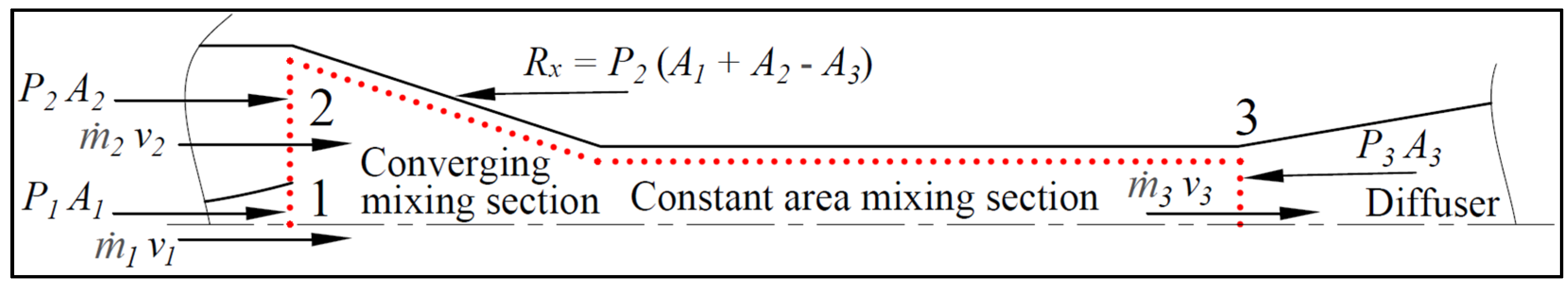
5. The One-Dimensional Analytical Model

In this section, the one-dimensional analytical model is presented. It is based on Al-Ansary’s work [9] with some re-arrangement. This will be in the first subsection. The ejector schematic drawing in Figure 1 is used for the derivation of the model. This analytical model will be referred to as the standard model. The equations are solved using Engineering Equation Solver (EES) [28]. Afterward, the modified one-dimensional analytical model is presented in the second subsection.

5.1. The Standard One-Dimensional Model

To simplify the one-dimensional ejector model, several common assumptions are made as shown below:

• The flow is one-dimensional and steady all over the ejector.
• The fluid is an ideal gas with constant specific heats (air is used in this work as the fluid).
• Friction at the walls is negligible.
• The kinetic energy at the inlet of primary flow, inlet of secondary flow and outlet of the ejector is negligible.
• The flow at the outlet of the primary nozzle is supersonic, i.e., the flow through the primary nozzle is choked. This assumption is merely based on the practical point of view, i.e., an ejector is usually required to operate at the critical conditions at which both primary and secondary flow are choked.
• The ejector is adiabatic, rigid (no boundary work involved), and impermeable (no flow entering or leaving the ejector besides flow through the inlets and outlet of the ejector).
• The isentropic efficiency of the primary nozzle and the subsonic diffuser (${\eta }_N$ and ${\eta }_D$) is known beforehand. In this work, the values are assumed to be constant with values of 0.95 and 0.8 for the nozzle and diffuser, respectively. These values are based on the typical efficiency of the devices. However, it should be kept in mind that actually, these fixed values of efficiency cannot be applied in all operating conditions of an ejector, and they will be one of the sources of error in the model. Therefore, a study to estimate the efficiencies of the nozzle and especially, the diffuser should be conducted in the future. By doing so, their efficiencies can be estimated more accurately by just knowing the geometry and operating conditions of the ejector.
• For an ejector that operates in the critical mode, a normal shock is assumed to happen at the exit of the mixing section (station 3). Therefore, the Mach number at that location, $M_3$, will be an input and have a value of one. For an ejector that operates in the sub-critical mode, the outlet static pressure, $P_4$, will be an input while the $M_3$ will be an output. However, in this work, the focus will be on the critical mode operation and, therefore, $M_3=1$ will act as an input and $P_4$ as an output. It should be noted that this assumption ($M_3=1$) has been found to be inaccurate at certain operating conditions. Yet, it is simple to apply and is thought to be a good initial approximation. In fact, the value of $M_3$ can either be greater or less than one, depending on where the shock starts. This is a challenge that remains to be solved.

The main targets of this model are to obtain the ${\dot{m}}_s$, ${\dot{m}}_p$, and $P_4$. The given/known parameters are as follows:

• The primary and secondary stagnation conditions (i.e., properties at station 0 and 2 in Figure 1).
• Ejector geometry:
  • Primary nozzle: Throat diameter, $D_{th}$, and outlet diameter, $D_1$.
  • Converging mixing section: Inlet diameter, $D_{CV,in}$.
  • Constant area mixing section (ejector throat): Diameter, $D_3$.
• Either the $M_3=1$ (for critical mode operation) or the $P_4$ (for sub-critical mode operation). However, the current work will focus on the critical mode operation of an ejector and, therefore, $M_3=1$ will act as an input and $P_4$ will be an output (assumption no. 8).
• The values of ${\eta }_N$ and ${\eta }_D$ are 0.95 and 0.8, respectively (assumption no. 7).

The governing equations (continuity, momentum, and energy balance equations), as well as equation of state of an ideal gas, will be applied whenever needed to construct the model. There are five control volumes required to develop the model and these control volumes will be shown in Figure 10, Figure 11 and Figure 12.

For control volume A shown in Figure 10, the mass and energy balance will be applied. The mass balance will result in Equation (5).

$${\dot{m}}_4={\dot{m}}_3={\dot{m}}_p+{\dot{m}}_s=\left(1+ER\right){\dot{m}}_p$$

(5)

where $ER$ stands for entrainment ratio and defined as

$$ER={\dot{m}}_s/{\dot{m}}_p$$

(6)

In order to obtain ${\dot{m}}_p$, the compressible flow equation for a choked flow (assumption no. 5) is used as presented in Equation (7) below.

$${\dot{m}}_p=A_{th} P_0\sqrt{\frac{\gamma }{R{T}_0}}{\left[\frac{2}{\gamma +1}\right]}^{\frac{\gamma +1}{2\left(\gamma -1\right)}}$$

(7)

where $\gamma$ and $R$ are the specific heat ratio and gas constant of air and have values of 1.4 and 287 J/kg-K, respectively. The $A_{th}$ denotes the primary nozzle throat area. The energy balance applied to the control volume A in conjunction with assumptions no. 2 and 4 gives Equation (8).

$$(T_0+ ER T_2)=\left(1+ER\right)T_4$$

(8)

Up to now, there are five unknowns, i.e., $ER$, ${\dot{m}}_p$, ${\dot{m}}_s$, ${\dot{m}}_4$, and $T_4$ and four equations which are Equations (5) to (8). Thus, another equation is needed to solve for these five unknowns. This equation will be obtained later via control volumes C and D.

Next, control volume B, also shown in Figure 10, will be considered. Through this control volume, the velocity, pressure, and Mach number at the outlet of the primary nozzle, denoted by $v_1$, $P_1$, and $M_1$, respectively, will be found. Applying energy balance to control volume B along with assumptions no. 2, 4, and 7, we will obtain Equation (9).

$$v_1=\sqrt{2 {\eta }_N c_{p } T_0 \left[1-{\left(\frac{P_1}{P_0}\right)}^{\frac{\gamma -1}{\gamma }}\right]}$$

(9)

As stated in assumption no. 7, the isentropic efficiency of the primary nozzle, ${\eta }_N$, is given which is assumed to be 0.95. However, there are two unknowns ($v_1$ and $P_1$) and only one equation, i.e., Equation (9). Thus, we need another equation.

To obtain another equation, the area ratio relation of isentropic compressible flow will be used as follows. Mach number at the outlet of the primary nozzle (station 1), $M_1$, can be calculated from (assuming there is no boundary layer separation between the throat and primary nozzle outlet):

$$\frac{A_1}{A_{th}}=\frac{1}{M_1}{\left[\frac{2}{\gamma +1}\left(1+\frac{\gamma -1}{2} M_1^2\right)\right]}^{\frac{\gamma +1}{2\left(\gamma -1\right)}}$$

(10)

where $A_1$ is the area at station 1 (the cross sectional area of the primary nozzle outlet). Hence, the pressure at the nozzle outlet, $P_1$, can be obtained from

$$\frac{P_0}{P_1}= {\left[1+\frac{\gamma -1}{2} M_1^2\right]}^{\frac{\gamma }{\gamma -1}}$$

(11)

Now, there are three unknowns and three equations which are $v_1$, $P_1$, and $M_1$ and Equations (9) to (11). Therefore, these parameters can be found.

For control volume C (see Figure 11 above and Figure 13 below), momentum equation will be applied to obtain a useful equation. It should be noted that the area at station 1, $A_1$, and station 2, $A_2$, are not overlapping. Area at station 1 is the outlet area of the primary nozzle and station 2 is the annulus area of the inlet of the converging mixing section. Thus, the total area at the inlet plane of control volume C is $A_1+A_2$ which is also referred to as the inlet area of the converging mixing section, $A_{CV,in}$.

The Newton second law states that the sum of forces acting on an object should be equal to the time rate of change of momentum of that object. This statement transforms to the following equation:

$$P_1{A}_1+P_2{A}_2-P_3{A}_3-R_x={\dot{m}}_3{v}_3-\left({\dot{m}}_p{v}_1+{\dot{m}}_s{v}_2\right)$$

(12)

where

$$R_x=P_{CV,w,avg}\left(A_1+A_2-A_3\right)$$

(13)

In this equation, $R_x$ and $P_{CV,w,avg}$ are the x-direction of the reaction force and average static pressure on control volume C, respectively, done by the wall of the converging mixing section. It should be noted that this pressure is averaged (area-weighted) based on the x-direction of the reaction force and x-direction of the converging wall area. Also, note that ${\dot{m}}_p$ and ${\dot{m}}_s$ (Equation (12)) are equal to ${\dot{m}}_1$ and ${\dot{m}}_2$ (Figure 13), respectively.

If it is assumed that the average static pressure on the wall of the converging mixing section is equal to the static pressure at station 2, then the reaction force in the x-direction, $R_x$, can be written as $R_x=P_2\left(A_1+A_2-A_3\right)$. This is illustrated in Figure 13. It should be noted that $P_2$ has also been assumed previously to be equal to the stagnation pressure of the secondary flow inlet. Recall assumption no. 4 where $v_2$ is assumed to be negligible and, thus, $P_2$ is the stagnation pressure at station 2.

Manipulating Equation (12) in conjunction with Equations (5), (6), (13), and the assumption of $P_{CV,w,avg}$ equals $P_2$, the following equation, Equation (14), will be found.

$${\dot{m}}_p{v}_1+P_1{A}_1+P_2(A_3-A_1)={\dot{m}}_p\left(1+ER\right)v_3+P_3{A}_3$$

(14)

After that, Equation (15) is obtained by applying the mass conservation across station 3 along with the ideal gas equation of state.

$$P_3{A}_3=\frac{{\dot{m}}_p\left(1+ER\right)R{T}_3}{v_3}$$

(15)

If the previous equations, i.e., Equations (5) to (8), are considered in conjunction with Equations (14) and (15), the number of unknowns will be eight while the number of equations will be six. The unknowns are $ER$, ${\dot{m}}_p$, ${\dot{m}}_s$, ${\dot{m}}_4$ (or ${\dot{m}}_3$), $T_4$, $v_3$, $T_3$, and $P_3$. Note that $v_1$ and $P_1$ are not included because they have been obtained before through Equations (9) to (11). Therefore, to solve these eight unknowns, two more equations are needed and one of them can be obtained from control volume D (Figure 12). The other equation is found based on the definition of Mach number and the assumption of knowing the value of $M_3$ (assumption no. 8).

Applying energy balance on control volume D together with assumptions no. 2 and 4, Equation (16) is obtained.

$$c_p T_o+ ER c_p T_2=\left(1+ER\right)\left(c_p T_3+\frac{v_3^2}{2}\right)$$

(16)

Using the definition of Mach number at station 3, we will get Equation (17).

$$v_3=M_3\sqrt{\gamma R{T}_3}$$

(17)

Thus, now, the system of equations is closed with eight equations (Equations (5) to (8) and Equations (14) to (17)) and eight unknowns ($ER$, ${\dot{m}}_p$, ${\dot{m}}_s$, ${\dot{m}}_4$ (or ${\dot{m}}_3$), $T_4$, $v_3$, $T_3$, and $P_3$).

Control volume E, i.e., the diffuser (Figure 12), will be used to get the last equation that will solve for pressure at the diffuser outlet (i.e., the ejector outlet), $P_4$. Applying energy balance on this control volume along with assumptions no. 2, 4, and 7, we will obtain Equation (18).

$$T_4=T_4{\left(\frac{P_3}{P_4}\right)}^{\frac{\gamma -1}{\gamma }}+\frac{v_3^2 {\eta }_D}{2c_{p }}$$

(18)

Hence, by using Equation (18), we can get the value of $P_4$ since all other parameters have been obtained previously. Recalling assumption no. 7, the diffuser isentropic efficiency, ${\eta }_D$, is known and assumed to have a value of 0.8.

5.2. The Modified One-Dimensional Model

The modified one-dimensional analytical model has the same set of equations as that of the standard model except on the converging mixing section wall pressure. The converging wall pressure ($P_{CV,w,avg}$) used to calculate the reaction force, $R_x$, in Equations (12) and (13) is not anymore assumed to equal $P_2$. Instead, the “actual” average wall pressure values will be utilized. These average pressure values are obtained from the CFD simulations. To find out if the converging wall pressure has a significant effect on the one-dimensional model results, these average wall pressure values from the CFD results are directly substituted into the equation. The flow chart of the model is shown in Figure 14.

6. Results and Discussion

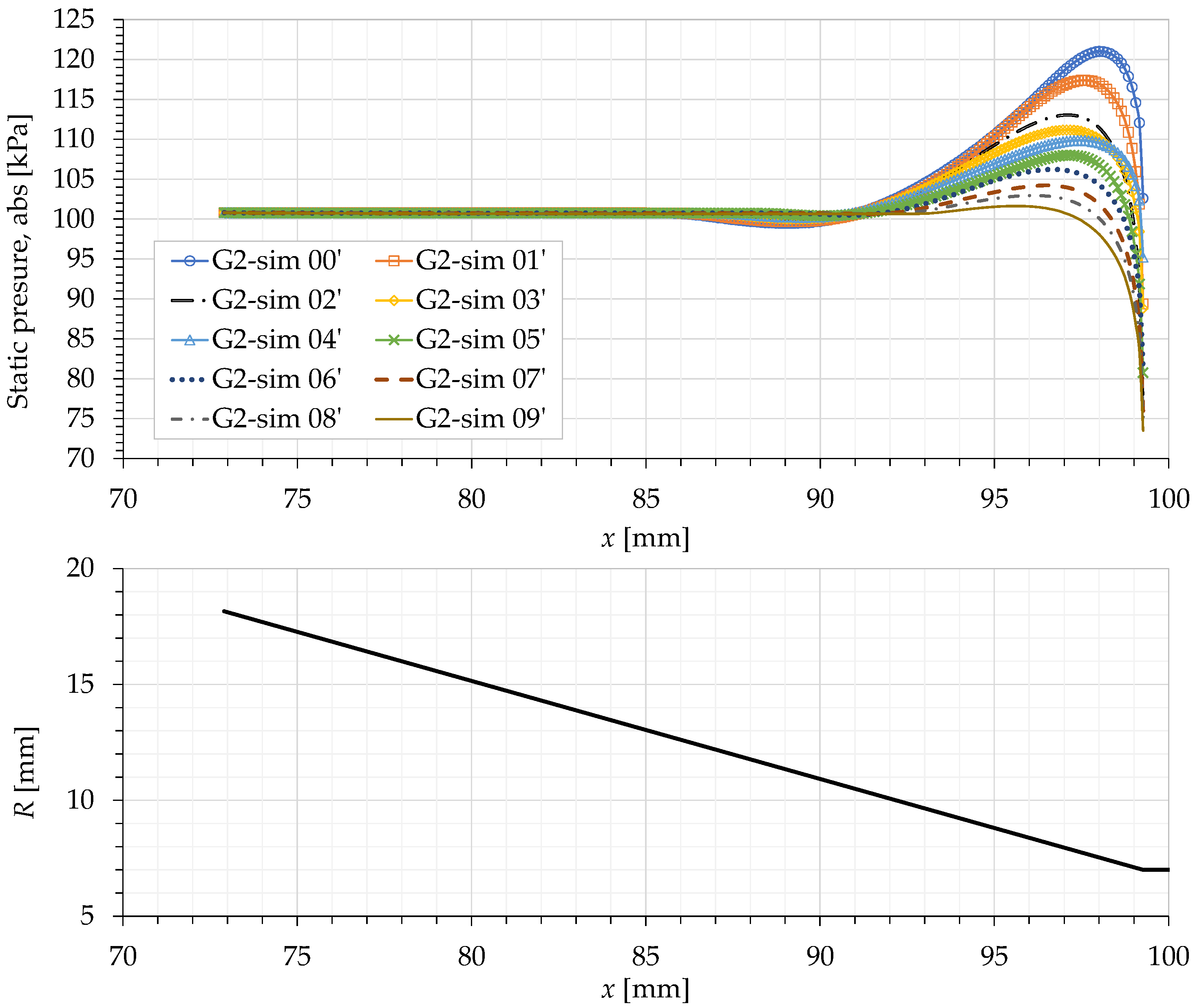
6.1. Pressure Variation on the Wall of the Converging Mixing Section

Figure 15 shows the pressure variation along the wall of the converging mixing section (80.7 ≤ $x$ ≤ 110 mm) of ejector G1. The wall of the converging mixing section consists of two contour patterns. One is the linear/straight contour with a steeper slope (80.7 mm ≤ $x$ ≤ 97 mm) and the other is the curved contour with a decreasing slope (97 mm ≤ $x$ ≤ 110 mm).

In general, all these pressure curves have the same pattern. They start to increase to reach a peak and then decrease, except for some curves, most notably the curves of sim 01 and 02. Note that the operating conditions for sim 00 to 09 in Figure 15 correspond to simulation no. 0 to 9 in Table 3, respectively. After the peak, these two curves decrease relatively a little and then increase again to finally decrease. Hence, there are two peaks. Such a pattern also exists, but is less obvious, in sim 03 and 05. This different pattern (the two peaks pattern) is mainly because of the different position and size of the shock train cells. Figure 16 compares simulation results having one peak pressure variation (sim 00) to that having two peaks (sim 01). The first pressure peak that occurs on the converging wall is due to the impingement of the secondary flow on the wall. After the impingement, part of the fluid flows into the ET and the remaining diverted into the steep converging wall to form a circulation. Regarding the second peak that exists on the other curves (ex: sim 01 in Figure 15), it is due to the different position and size of the cells of the shock train. The outer surface of the shock train and the ejector wall create a hypothetical annular duct that is continuously expanding and contracting along the $x$-direction. When the cross-sectional area of this annular duct increases (the duct diverges), the flow inside it will decelerate and, hence, the wall pressure increases (see the second pressure peak in Figure 16). The opposite will happen if the cross-sectional area of the duct decreases (the duct converges). A similar phenomenon is also seen in the flow of ejectors G2, G2.1, and G2.2, which will be presented next.

In the parametric study, the standard and the modified one-dimensional models were applied to the three ejectors (G2, G2.1, and G2.2), and the results were compared. All these ejectors were simulated at the critical conditions ($P_0\ge$ 308 kPa). The results of the modified model are encouraging. From Figure 17, Figure 18 and Figure 19, there are two important observations to point out. Firstly, looking at the curves in general, one can see that the ${\dot{m}}_s$ from CFD simulation decreases as the $P_0$ increases. This means that it has a negative slope. On the other hand, the standard model shows the opposite, i.e., a positive slope. However, the curve slope of the modified model gets closer to that of the CFD results. This means that the one-dimensional model is improved. The second observation to point out is that, at high $P_0$, the modified model improves the prediction of ${\dot{m}}_s$ significantly. Interestingly, such improvement is obtained by only a slight change in the average pressure of the converging mixing section wall as can be seen in

Table 5. The discrepancy (in percent) between the ${\dot{m}}_s$ obtained from the one-dimensional analytical models (std and mod) and CFD for various ejectors.

Sim no.	${\mathit{P}}_0 \left[\mathbf{kPa}\right]$	Ejector G2			Ejector G2.1			Ejector G2.2
		∆PCV 1 [%]	${\dot{m}}_{s,1D}$2 [%]		∆PCV 1 [%]	${\dot{m}}_{s,1D}$2 [%]		∆PCV 1 [%]	${\dot{m}}_{s,1D}$2 [%]
			1-D, std	1-D, mod		1-D, std	1-D, mod		1-D, std	1-D, mod
0’	618	1.91	43.43	11.84	2.85	41.03	12.62	3.87	30.47	13.41
1’	584	1.61	27.86	2.91	2.32	24.82	3.30	2.96	17.20	4.90
2’	549	1.19	9.39	−7.19	1.62	6.42	−7.00	1.79	1.89	−4.89
3’	515	1.11	2.77	−12.57	1.49	−0.08	−12.39	1.11	−8.51	−12.54
4’	480	1.01	−2.45	−16.53	1.34	−4.93	−16.11	1.33	−10.79	−15.81
5’	446	0.64	−14.59	−22.90	0.72	−16.49	−22.09	0.39	−19.57	−20.97
6’	412	0.42	−22.28	−27.60	0.33	−24.69	−27.19	−0.84	−29.18	−26.40
7’	377	0.13	−30.00	−31.54	−0.08	−31.61	−31.03	−1.22	−34.30	−30.23
8’	343	−0.06	−36.01	−35.29	−0.36	−37.28	−34.73	−1.72	−39.55	−33.88
9’	308	−0.28	−42.85	−39.55	−0.70	−43.91	−39.02	−2.25	−45.56	−38.28

¹$∆P_{CV}=\left(P_{CV,w,avg}-P_2\right)\times 100/P_2 [\%]$; where $P_2$ = 100.8 kPa and $P_{CV,w,avg}$ is the average wall pressure of the converging mixing section obtained from CFD. ² $∆{\dot{m}}_{s,1D}=\left({\dot{m}}_{s,1D}-{\dot{m}}_{s,CFD}\right)\times 100/{\dot{m}}_{s,CFD} [\%]$; ${\dot{m}}_{s,1D}$ and ${\dot{m}}_{s,CFD}$ are the secondary mass flow rates obtained from the one-dimensional model and CFD, respectively.

. As an example, for simulation no. 0’ of ejector G2, a pressure difference of only 1.91% leads to 31.59% improvement on the one-dimensional model prediction of the secondary mass flow rate.

The fact that there is only a slight improvement at lower $P_0$ leads to the following conclusions. Firstly, the pressure variation on the converging wall is too small which means that the average (area-weighted) pressure is close to $P_2$. This can be seen in Table 5 above. Secondly, it means that other phenomena, which are beyond the scope of this research, play a more significant role in this pressure region. Despite the slight improvement in the lower $P_0$ region, it is important to note that the one-dimensional prediction of ${\dot{m}}_s$ is very sensitive to the change of the converging wall pressure, regardless what the $P_0$ values are. Figure 20 helps to explain the statement.

In Figure 20, $∆P_{CV}$ has the same definition as that in Table 5. The ${\dot{m}}_{s,1D,mod-std}$ is defined as $\left({\dot{m}}_{s,1D,mod}-{\dot{m}}_{s,1D,std}\right)\times 100/{\dot{m}}_{s,CFD}$ in percent where ${\dot{m}}_{s,CFD}$ is the secondary mass flow rate obtained from CFD, and ${\dot{m}}_{s,1D,std}$ and ${\dot{m}}_{s,1D,mod}$ are the secondary mass flow rates obtained from the standard and modified one-dimensional models, respectively. In this figure, it can be concluded that the least sensitive ejector to wall pressure change is ejector G2.2. Yet, it is still something that cannot be ignored even at lower pressures. As an example, for the lowest $P_0$ (308 kPa), when the converging wall pressure decreases by 2.25%, the predicted mass flow rate increases by 7.28%. The most sensitive to the wall pressure change is ejector G2. At the lowest $P_0$ (308 kPa), an only 0.28% decrease in the wall pressure results in 3.30% increase in the predicted mass flow rate.

These results suggest that, instead of simply assuming $P_{CV,w,avg}$ to be equal to $P_2$, a good estimate of the pressure should be found and utilized. This finding also proves what has been suggested by Little and Garimella [1], i.e., more local flow phenomena should be included in the one-dimensional model to improve it further.

Figure 21 and Figure 22 are presented to show how the pressure varies along the converging mixing section wall for ejector G2 and G2.1, respectively. Ejector G2.2 results are similar; hence, they are not presented here. Like what has been observed in ejector G1, the pressure starts to vary when the primary flow jet gets closer to the wall. The pressure initially increases to reach a peak and then decreases as the flow is about to enter the throat. This is because the secondary flow impinges the converging wall as can be seen in Figure 23, hence the peak in the pressure variation curve. Around this region, the pressure is at maximum. The impinging flow is then divided into two streams; one enters the ET and the other stream diverts to the converging wall and forms circulation. Such flow circulation has been observed by Han et al. [25] in their CFD simulations.

Paying attention again to Figure 21 and Figure 22, one can see that the curve peak (“mountain” curve size) decreases gradually as the $P_0$ decreases. It is also observed that the curve pattern for simulation no. 4’ (sim 04’) is rather different, i.e., the decrease in wall pressure after the peak is not as steep as the others. The explanation for these two phenomena (the gradual decrease of the “mountain” curve size and “anomaly” of sim 04’ curve) is as follows in conjunction with Figure 24. At higher $P_0$, the secondary flow has higher momentum as it enters the ejector. This is because the shear effect between the two flows (primary and secondary) gets stronger. However, due to the larger diameter of the shock cell, the secondary flow will not be able to directly enter the ejector throat. Rather, it will impinge the converging mixing section wall before the flow divided into two streams (Figure 23) as explained before. Thus, the dynamic pressure (kinetic energy) will be converted to pressure as the flow hits the wall. The higher the momentum of the secondary flow is, the higher the pressure at the converging wall will be, and vice versa. This explains the gradual decrease in the “mountain” size in the two figures as the $P_0$ decreases.

Regarding the “anomaly” of simulation no. 4’ (sim 04’), it is related to the shock cells position and size inside the ejector, particularly in this case, inside the converging mixing section. Looking at sim 04’ in Figure 24, one can see that the end of one of the shock cells is located just before the ET inlet. Thus, the hypothetical annular duct formed is diverging. This will hinder the flow to accelerate. The decrease in the flow acceleration shows up in the pressure curve of sim 04’ as a less steep pressure drop after the peak. Observing the Mach contour plot of the other simulations in this figure, it is clearly seen that the hypothetical annular duct near the ET inlet is converging and, therefore, the pressure drop in the curve is steeper because the flow has higher acceleration.

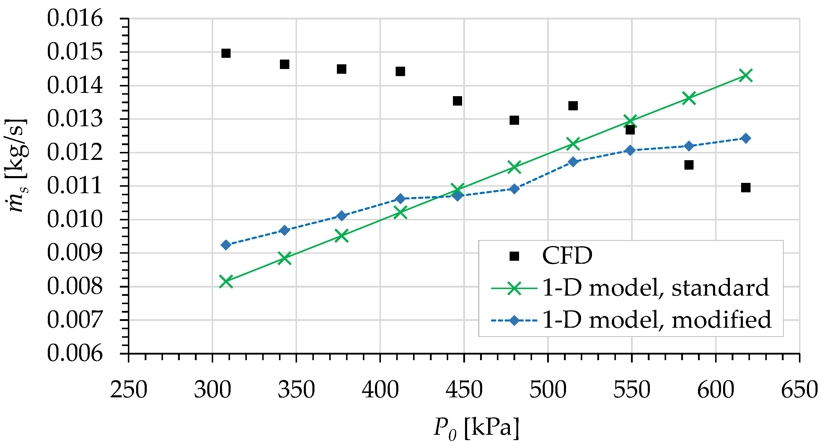
6.2. Secondary Mass Flow Rate Comparison

The effect of reducing the radius of the converging mixing section inlet, $R_{CV,in}$, is analyzed. Reducing this radius means that the angle of the converging mixing section is reduced. The angles for ejector G2, G2.1, and G2.2 are 22.94°, 16.60°, and 9.60°, respectively.

The CFD results show that the secondary mass flow rate increases as the radius decreases or, in other words, as the angle decreases. This trend can be seen in

Table 6. Comparison of secondary mass flow rates from CFD simulation for ejectors having different inlet radius/converging angle of the converging mixing section.

Sim. no.	${\mathit{P}}_0 \left[\mathbf{kPa}\right]$	$\mathbf{Sec}\mathbf{ondary} \mathbf{Mass} \mathbf{Flow} \mathbf{Rate}, {\dot{\mathit{m}}}_{\mathit{s}} [\mathbf{kg}/\mathbf{s}]$			$\mathbf{Increase} \mathbf{of} {\dot{\mathit{m}}}_{\mathit{s}} \mathbf{Relative} \mathbf{to} \mathbf{that} \mathbf{of} \mathbf{Ejector} \mathbf{G}2 [\%]$
		Ejector G2	Ejector G2.1	Ejector G2.2	Ejector G2.1	Ejector G2.2
0’	618	0.00997	0.01014	0.01096	1.71	9.93
1’	584	0.01066	0.01092	0.01163	2.44	9.10
2’	549	0.01182	0.01215	0.01269	2.79	7.36
3’	515	0.01193	0.01227	0.01340	2.85	12.32
4’	480	0.01186	0.01217	0.01297	2.61	9.36
5’	446	0.01275	0.01304	0.01354	2.27	6.20
6’	412	0.01315	0.01357	0.01443	3.19	9.73
7’	377	0.01360	0.01392	0.01449	2.35	6.54
8’	343	0.01383	0.01411	0.01464	2.02	5.86
9’	308	0.01426	0.01453	0.01497	1.89	4.98

. The finding agrees with that of Jeong et al. [30], however, they have found an optimum angle which will result in a maximum ${\dot{m}}_s$. Thus, the ${\dot{m}}_s$ keeps increasing as the angle decreases until it reaches a certain angle (the optimum angle). A further decrease in the angle will decrease the ${\dot{m}}_s$.

In the current work, such an optimum angle of converging mixing section has not been found because, most likely, the range of the angle variation is not wide enough. Jeong et al. [30] concluded that the optimum angle is 1° while the ejector considered in the current research has a minimum angle of 9.60°. Moreover, the dimension of the other parts of their ejector is different which may cause the difference in the optimum angle. Zhu et al. [18] have also found an optimum converging mixing section angle. Their results show that the optimum angle cannot be generalized to meet all operating conditions. Therefore, they suggested that research to develop an adjustable ejector should be conducted, especially an ejector with an adjustable primary nozzle exit position and adjustable converging mixing section angle.

7. Conclusions

A research on supersonic ejectors for refrigeration application using computational fluid dynamics (CFD) and one-dimensional analytical models has been conducted. Several ejectors with varying radius of converging mixing section inlet were studied. The objective was to show that the ejector one-dimensional analytical model can be improved by considering wall pressure variation in the converging mixing section. Typically, the pressure on this wall is assumed to be constant and equal to the secondary flow inlet pressure. Two turbulence models, i.e., k-omega SST and transition SST, have been tested to find which one gives the closest results to the experimental data. The predicted secondary mass flow rates, ${\dot{m}}_s$, obtained from the one-dimensional model have been compared before and after incorporating the above-mentioned pressure variation into the model.

The conclusions of this work are summarized as follows:

• In the CFD analysis, the transition SST turbulence model is better than the k-omega SST model in terms of how close the predicted ${\dot{m}}_s$ is to the experimental data. Most of the transition SST model results are within the experimental uncertainty of Al-Ansary’s work [9], i.e., no greater than 4%. On the other hand, many of the errors of k-omega SST results are ranging from 7% to 9%. These results are obtained when the ejector is operating in the critical region.
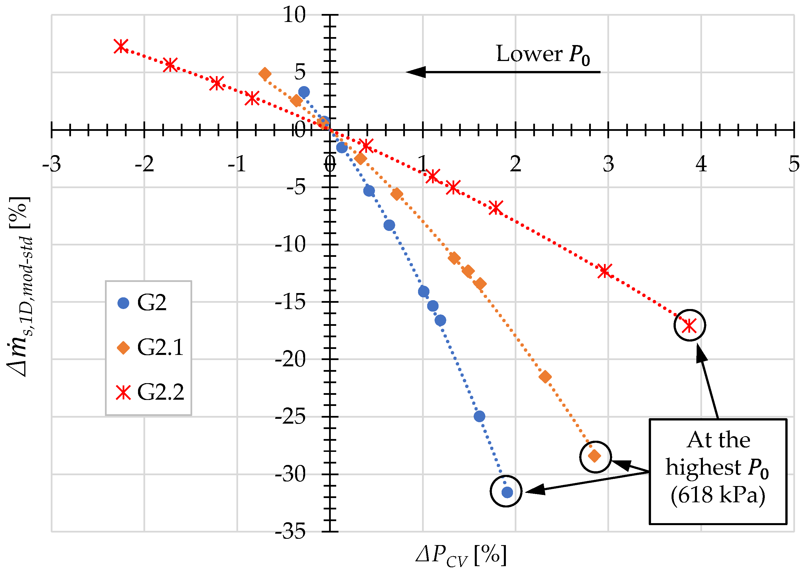
• The authors have found that the effect of wall pressure variation in the converging mixing section is actually prominent in the prediction of the one-dimensional model. Even a small amount of change in the converging wall pressure can result in a significant improvement of the model prediction of ${\dot{m}}_s$, especially at high $P_0$. However, regardless of the operating conditions, the sensitivity of ${\dot{m}}_s$ is high with respect to the change of the converging wall pressure, i.e., a small change in the pressure can result in a high change in ${\dot{m}}_s$. It has also been found that, in general, the inclusion of the wall pressure variation will improve the trend (slope) of the predicted ${\dot{m}}_s$. Based on these findings, this wall pressure variation should be considered in future modeling of ejectors.
• The pressure increase on the wall of the converging mixing section is due to the impingement of the secondary flow on that wall. This happens because the shock train of the primary jet partially blocks the secondary flow as it tries to enter the ET. On the other hand, the pressure decrease at the end of that converging wall is due to the acceleration of the secondary flow as it enters the ET. The effects of these two phenomena compete each other that result in the increase or decrease of the average wall pressure. Moreover, we have also found that the behaviors of these two phenomena are linked to the primary jet speed, and the cell size and position of the shock train.
• The CFD results show that the secondary mass flow rate increases as the angle of the converging mixing section decreases. However, due to the limited range of angles simulated, the current results have not verified the existence of an optimum angle value that has been observed by other researchers.

The future work will be an effort to compare other different ejector geometries and to obtain a mathematical relation that links the operating conditions ($P_0$, $P_2$, and $P_4$) and ejector geometry to the pressure of the converging mixing section wall. Moreover, other local flow phenomena should be analyzed to find out which ones that have significant effects on the one-dimensional model.

References

1. Little, A.B.; Garimella, S. A critical review linking ejector flow phenomena with component- and system-level performance. Int. J. Refrig. 2016, 70, 243–268. [Google Scholar] [CrossRef]
2. Huang, B.J.; Chang, J.M.; Wang, C.P.; Petrenko, V.A. A 1-D analysis of ejector performance. Int. J. Refrig. 1999, 22, 354–364. [Google Scholar] [CrossRef]
3. Keenan, J.H.; Neumann, E.P. A Simple Air Ejector. J. Appl. Mech. Trans. ASME 1942, 9, A75–A81. [Google Scholar]
4. Keenan, J.H.; Neumann, E.P.; Lustwerk, F. An investigation of ejector design by analysis and experiment. J. Appl. Mech. Trans. ASME 1950, 17, 299–309. [Google Scholar]
5. Chen, W.; Liu, M.; Chong, D.; Yan, J.; Little, A.B.; Bartosiewicz, Y. A 1D model to predict ejector performance at critical and sub-critical operational regimes. Int. J. Refrig. 2013, 36, 1750–1761. [Google Scholar] [CrossRef]
6. Chen, W.; Liu, M.; Chong, D.; Yan, J.; Little, A.B.; Bartosiewicz, Y. Corrigendum to “A 1D model to predict ejector performance at critical and sub-critical operational regimes” [JIJR 36/6 (2013) 1750–1761]. Int. J. Refrig. 2017, 75, 177. [Google Scholar] [CrossRef]
7. Kumar, N.S.; Ooi, K.T. One dimensional model of an ejector with special attention to Fanno flow within the mixing chamber. Appl. Therm. Eng. 2014, 65, 226–235. [Google Scholar] [CrossRef]
8. Zhu, Y.; Cai, W.; Wen, C.; Li, Y. Shock circle model for ejector performance evaluation. Energy Convers. Manag. 2007, 48, 2533–2541. [Google Scholar] [CrossRef]
9. Al-Ansary, H.A.M. Investigation and Improvement of Ejector-Driven Heating and Refrigeration Systems. Ph.D. Thesis, Georgia Institute of Technology, GA, USA, 2004. [Google Scholar]
10. Al-Ansary, H.A. A Semi-Empirical One-Dimensional Model for Flow in Ejectors Used for Gas Evacuation. In Proceedings of the Fluids Engineering Division Summer Meeting, Miami, FL, USA, 17–20 July 2006; pp. 41–48. [Google Scholar] [CrossRef]
11. Al-Ansary, H.A.M.; Jeter, S.M. Numerical and Experimental Analysis of Single-Phase and Two-Phase Flow in Ejectors. HvacR Res. 2004, 10, 521–538. [Google Scholar] [CrossRef]
12. Mazzelli, F.; Little, A.B.; Garimella, S.; Bartosiewicz, Y. Computational and experimental analysis of supersonic air ejector: Turbulence modeling and assessment of 3D effects. Int. J. Heat Fluid Flow 2015, 56, 305–316. [Google Scholar] [CrossRef]
13. Pianthong, K.; Seehanam, W.; Behnia, M.; Sriveerakul, T.; Aphornratana, S. Investigation and improvement of ejector refrigeration system using computational fluid dynamics technique. Energy Convers. Manag. 2007, 48, 2556–2564. [Google Scholar] [CrossRef]
14. Bartosiewicz, Y.; Aidoun, Z.; Desevaux, P.; Mercadier, Y. Numerical and experimental investigations on supersonic ejectors. Int. J. Heat Fluid Flow 2005, 26, 56–70. [Google Scholar] [CrossRef]
15. Besagni, G.; Inzoli, F. Computational fluid-dynamics modeling of supersonic ejectors: Screening of turbulence modeling approaches. Appl. Therm. Eng. 2017, 117, 122–144. [Google Scholar] [CrossRef]
16. Croquer, S.; Poncet, S.; Aidoun, Z. Turbulence modeling of a single-phase R134a supersonic ejector. Part 1: Numerical benchmark. Int. J. Refrig. 2016, 61, 140–152. [Google Scholar] [CrossRef]
17. Ruangtrakoon, N.; Thongtip, T.; Aphornratana, S.; Sriveerakul, T. CFD simulation on the effect of primary nozzle geometries for a steam ejector in refrigeration cycle. Int. J. Therm. Sci. 2013, 63, 133–145. [Google Scholar] [CrossRef]
18. Zhu, Y.; Cai, W.; Wen, C.; Li, Y. Numerical investigation of geometry parameters for design of high performance ejectors. Appl. Therm. Eng. 2009, 29, 898–905. [Google Scholar] [CrossRef]
19. Zhu, Y.; Jiang, P. Experimental and numerical investigation of the effect of shock wave characteristics on the ejector performance. Int. J. Refrig. 2014, 40, 31–42. [Google Scholar] [CrossRef]
20. Hemidi, A.; Henry, F.; Leclaire, S.; Seynhaeve, J.-M.; Bartosiewicz, Y. CFD analysis of a supersonic air ejector. Part I: Experimental validation of single-phase and two-phase operation. Appl. Therm. Eng. 2009, 29, 1523–1531. [Google Scholar] [CrossRef] [Green Version]
21. Hemidi, A.; Henry, F.; Leclaire, S.; Seynhaeve, J.-M.; Bartosiewicz, Y. CFD analysis of a supersonic air ejector. Part II: Relation between global operation and local flow features. Appl. Therm. Eng. 2009, 29, 2990–2998. [Google Scholar] [CrossRef] [Green Version]
22. Wang, L.; Yan, J.; Wang, C.; Li, X. Numerical study on optimization of ejector primary nozzle geometries. Int. J. Refrig. 2017, 76, 219–229. [Google Scholar] [CrossRef]
23. Sriveerakul, T.; Aphornratana, S.; Chunnanond, K. Performance prediction of steam ejector using computational fluid dynamics: Part 1. Validation of the CFD results. Int. J. Therm. Sci. 2007, 46, 812–822. [Google Scholar] [CrossRef]
24. Dong, J.; Yu, M.; Wang, W.; Song, H.; Li, C.; Pan, X. Experimental investigation on low-temperature thermal energy driven steam ejector refrigeration system for cooling application. Appl. Therm. Eng. 2017, 123, 167–176. [Google Scholar] [CrossRef]
25. Han, Y.; Wang, X.; Sun, H.; Zhang, G.; Guo, L.; Tu, J. CFD simulation on the boundary layer separation in the steam ejector and its influence on the pumping performance. Energy 2019, 167, 469–483. [Google Scholar] [CrossRef]
26. Mohamed, S.; Shatilla, Y.; Zhang, T. CFD-based design and simulation of hydrocarbon ejector for cooling. Energy 2019, 167, 346–358. [Google Scholar] [CrossRef]
27. Varga, S.; Soares, J.; Lima, R.; Oliveira, A.C. On the selection of a turbulence model for the simulation of steam ejectors using CFD. Int. J. Low Carbon Technol. 2017, 12, 233–243. [Google Scholar] [CrossRef]
28. Klein, S.A. Engineering Equation Solver (EES); Commercial V10.933-3D.; F-Chart Software; Available online: http://fchartsoftware.com (accessed on 5 October 2020).
29. ANSYS Fluent User’s Guide, Release 19.0; ANSYS, Inc.: Canonsburg, PA, USA, 2018.
30. Jeong, H.; Utomo, T.; Ji, M.; Lee, Y.; Lee, G.; Chung, H. CFD analysis of flow phenomena inside thermo vapor compressor influenced by operating conditions and converging duct angles. J. Mech. Sci. Technol. 2009, 23, 2366–2375. [Google Scholar] [CrossRef]
Figure 1. Schematic of a typical ejector.
Applsci 11 03245 g001
Figure 2. Various ejector operation modes at a fixed primary and secondary inlet pressures. Entrainment ratio (the y-axis) is the ratio of secondary to primary mass flow rates.
Applsci 11 03245 g002
Figure 3. The internal contour of Al-Ansary’s ejector [9] (ejector G1) used for the computational fluid dynamics (CFD) validation in the current study.
Applsci 11 03245 g003
Figure 4. The zoomed-in ejector geometry around the converging mixing section. The base geometry for the parametric study, ejector G2, (solid grey lines) is superimposed on the geometry for the CFD validation, ejector G1, (the solid green lines connecting the green dots).
Applsci 11 03245 g004
Figure 5. The variation in ejector geometry for the parametric study.
Applsci 11 03245 g005
Figure 6. Absolute static pressure along the axis (top). The ejector internal contour (bottom) is also presented to see the corresponding location of the static pressure. The turbulence model is the transition SST model.
Applsci 11 03245 g006
Figure 7. The sample of the chosen mesh (medium mesh) around the exit of the primary nozzle as well as the inlet of the secondary flow is shown in (a) and the “Detail A” is shown in (b).
Applsci 11 03245 g007aApplsci 11 03245 g007b
Figure 8. Qualitative comparison of the non-dimensional wall pressure ( P w / P 2 ) along the mixing section up to the diffuser between Han et al.’s work (a) and the current work (turbulence model: transition SST; P 0 = 618 kPa) (b). The left figure (a) is reprinted from the work of Han et al. [25] with the wall pressure ( y -axis) is non-dimensionalized by the secondary inlet pressure of their work ( P 2 = 3170 Pa).
Applsci 11 03245 g008
Figure 9. The Mach number contour plot for M ≥ 1 showing the periodically constricted hypothetical annular duct (turbulence model: transition SST; P 0 = 618 kPa).
Applsci 11 03245 g009
Figure 10. The dashed (blue) line and dotted (red) lines are showing control volumes A and B, respectively.
Applsci 11 03245 g010
Figure 11. The dotted line is showing control volume C.
Applsci 11 03245 g011
Figure 12. The dotted (red) and dashed (blue) lines are showing control volumes D and E, respectively.
Applsci 11 03245 g012
Figure 13. Forces and momentum flow on control volume C.
Applsci 11 03245 g013
Figure 14. Flowchart of the one-dimensional model.
Applsci 11 03245 g014
Figure 15. Pressure variation along the wall of the converging mixing section (80.7 mm ≤ x ≤ 110 mm) of ejector G1 (top) and the geometrical contour of the converging mixing section wall (bottom). The operating conditions of sim 00 to 09 can be seen in Table 3 (corresponding to simulation no. 0 to 9).
Applsci 11 03245 g015
Figure 16. Streamlines plot (colored by pressure) started from the secondary flow inlet for ejector G1 with operating conditions of sim 00 ( P 0 = 618 kPa; top), and 01 ( P 0 = 584 kPa; bottom). Mach number contour lines of the primary flow for M 1 (black lines) are superimposed onto it to see the shock cells position and size.
Applsci 11 03245 g016
Figure 17. The secondary mass flow rates of ejector G2 obtained from various methods for different primary pressures.
Applsci 11 03245 g017
Figure 18. The secondary mass flow rates of ejector G2.1 obtained from various methods for different primary pressures.
Applsci 11 03245 g018
Figure 19. The secondary mass flow rates of ejector G2.2 obtained from various methods for different primary pressures.
Applsci 11 03245 g019
Figure 20. The effect of the converging wall pressure change on the change of the secondary mass flow rate obtained from the one-dimensional model.
Applsci 11 03245 g020
Figure 21. Pressure variation along the wall of the converging mixing section (72.9 ≤ x ≤ 99.259 mm) of ejector G2 (top) and the geometrical contour of the converging mixing section wall (bottom). The operating conditions of sim 00’ to 09’ can be seen in Table 5 (correspond to sim no. 0’ to 9’).
Applsci 11 03245 g021
Figure 22. Pressure variation along the wall of the converging mixing section (72.9 ≤ x ≤ 99.259 mm) of ejector G2.1 (top) and the geometrical contour of the converging mixing section wall (bottom). The operating conditions of sim 00’ to 09’ can be seen in Table 5 (correspond to sim no. 0’ to 9’).
Applsci 11 03245 g022
Figure 23. Streamlines plot (colored by pressure) started from the secondary flow inlet for ejector G2 with operating condition of simulation no. 0’ (Table 5), i.e., P 0 = 618 kPa.
Applsci 11 03245 g023
Figure 24. Mach number contour plot (M ≥ 1) of CFD results of ejector G2.1. The operating conditions of sim 00’ to 09’ can be seen in Table 5 (correspond to sim no. 0’ to 9’).
Applsci 11 03245 g024