
Large-Scale Truss-Sizing Optimization with Enhanced Hybrid HS Algorithm
by
 , , , and
Sadik Ozgur Degertekin
1,* ,
,
Mohammad Minooei
2 ,
,
Lorenzo Santoro
2,
Bartolomeo Trentadue
2 and
Luciano Lamberti
2,* 1
Department of Civil Engineering, Dicle University, 21280 Diyarbakir, Turkey
2
Dipartimento di Meccanica, Matematica e Management, Politecnico di Bari, 70125 Bari, Italy
*
Authors to whom correspondence should be addressed.
Appl. Sci. 2021, 11(7), 3270; https://0-doi-org.brum.beds.ac.uk/10.3390/app11073270
Submission received: 27 January 2021
/
Revised: 29 March 2021
/
Accepted: 31 March 2021
/
Published: 6 April 2021
(This article belongs to the Special Issue Harmony Search Algorithm - Theoretical Background and Practical Applications)
Abstract
:Metaheuristic algorithms currently represent the standard approach to engineering optimization. A very challenging field is large-scale structural optimization, entailing hundreds of design variables and thousands of nonlinear constraints on element stresses and nodal displacements. However, very few studies documented the use of metaheuristic algorithms in large-scale structural optimization. In order to fill this gap, an enhanced hybrid harmony search (HS) algorithm for weight minimization of large-scale truss structures is presented in this study. The new algorithm, Large-Scale Structural Optimization–Hybrid Harmony Search JAYA (LSSO-HHSJA), developed here, combines a well-established method like HS with a very recent method like JAYA, which has the simplest and inherently most powerful search engine amongst metaheuristic optimizers. All stages of LSSO-HHSJA are aimed at reducing the number of structural analyses required in large-scale structural optimization. The basic idea is to move along descent directions to generate new trial designs, directly through the use of gradient information in the HS phase, indirectly by correcting trial designs with JA-based operators that push search towards the best design currently stored in the population or the best design included in a local neighborhood of the currently analyzed trial design. The proposed algorithm is tested in three large-scale weight minimization problems of truss structures. Optimization results obtained for the three benchmark examples, with up to 280 sizing variables and 37,374 nonlinear constraints, prove the efficiency of the proposed LSSO-HHSJA algorithm, which is very competitive with other HS and JAYA variants as well as with commercial gradient-based optimizers.
1. Introduction
Metaheuristic optimization methods inspired by evolution theory, life sciences and zoology, physics and astronomy, human sciences, etc., are successfully utilized in science and engineering. For example, genetic algorithms (GA) [1], differential evolution [2], simulated annealing (SA) [3], particle swarm optimization (PSO) [4], ant colony optimization (ACO) [5], firefly algorithm (FFA) [6], cuckoo search (CS) [7], ant lion optimizer [8], Tabu search (TS) [9], harmony search (HS) [10], teaching-learning based optimization (TLBO) [11], JAYA [12], big bang-big crunch (BBBC) [13], charged system search (CSS) [14], ray optimization (RO) [15], colliding bodies optimization [16], water evaporation optimization (WEO) [17], cyclical parthenogenesis algorithm (CPA) [18], and coyote optimization algorithm (COA) [19] are representative metaheuristic methods with several variants documented in the optimization literature.
Generally speaking, optimization algorithms may be trajectory-based or population-based. In the former case, a single design is elaborated in each iteration, thus building a “trajectory” connecting the initial solution with the optimal solution and passing through all intermediate solutions found in each iteration. Trajectory-based algorithms include gradient-based methods using linear or quadratic approximations of the optimization problem as well as some metaheuristic algorithms such as, for example, simulated annealing, randomized local search and simplified variants of differential evolution. Population-based algorithms update a population of candidate solutions until the search process converges to the optimum design after a predefined number of iterations or function evaluations. This category practically includes all metaheuristic algorithms except those classified above as trajectory-based algorithms.
While metaheuristic algorithms practically became the standard approach to engineering optimization (see, for example, the review articles and books [20,21,22,23,24] focusing on structural optimization), the “no free lunch” theorem [25,26] had an important consequence in the fact that no metaheuristic algorithm can prove itself superior over all other algorithms in all problems. A general-purpose universal optimization algorithm does not exist from the theoretical point of view. However, an algorithm can outperform its competitors if it is specialized to the specific problem at hand. For this reason, most of the metaheuristic algorithms lost their appeal just after a very few years. This is not the case of Harmony Search (HS) [10], which was developed almost 20 years ago, but remains a very popular optimization algorithm.
The HS method is a population-based metaheuristic algorithm that simulates the process of searching for a perfect state of harmony performed by jazz players. The relationship of HS to music is well summarized in Yang [27]. Three possible options are available to a skilled musician who is improvising: (1) play any famous piece of music (a series of pitches in harmony) exactly from his or her memory; (2) play something similar to a known piece (thus adjusting the pitch slightly); (3) compose new or random notes. These three options were formalized by Geem et al. [10] into the harmony search optimization algorithm. A set of NPOP randomly generated solutions are stored in a matrix called harmony memory [HM]. New trial designs may be extracted from [HM] or randomly selected according to the value taken by the harmony memory considering rate (HMCR) parameter. Design variables may be modified according to the value taken by the pitch adjustment rate (PAR) parameter; the bandwidth parameter (bw) quantifies the amount of variation given to a variable in the pitch adjustment operation.
Structural optimization is an important field of engineering concerned with the optimum design of structures [28,29,30]. The most common goal in structural optimization is to minimize the weight of the structure in the presence of limitations on deformations, stresses, critical loads, natural frequencies, etc. However, other objectives can be considered such as, for example, to minimize stresses or maximize stiffness. Structural optimization problems may be of three types: (i) sizing optimization where design variables correspond to geometric dimensions such as, for example, the cross-sectional areas of the elements forming the structure; (ii) shape optimization where design variables define the profile of the structure (e.g., coordinates of nodes); (iii) topology optimization where design variables define the distribution of the material in the structure.
The easiness of implementation of HS soon attracted many structural optimization experts that developed several variants of the algorithm after the pioneering studies by Lee and Geem [31,32]. In particular, researchers attempted to (i) minimize the sensitivity of convergence behavior to the setting of HMCR, PAR and bw parameters; (ii) reduce the number of structural analyses and speed up the search process by removing trial solutions yielding no improvements in design. These abilities turn very useful, especially in the optimization of large-scale structures. For example, Saka [33] used an adaptive error strategy to handle slightly infeasible designs. Maheri and Narimani [34] considered designs deemed worse than the worst design stored in [HM], yet distant from local optima. Murren and Khandelwal [35] generated random trial solutions within intelligently specified search neighborhoods. Mahdavi et al. [36] dynamically updated the PAR and bw parameters in the search process, while Carbas and Saka [37] used another dynamic scheme for updating the HMCR and PAR parameters. Hasancebi et al. [38] probabilistically selected HS parameters to the adapt search to varying features of design space. A self-adaptive HS algorithm also implemented by Degertekin [39]. Kaveh and Naiemi [40] developed a multi-adaptive HS variant updating internal parameters linearly or exponentially. Geem and Sim [41] developed a parameter-setting-free technique selecting specific operators for each variable stored in [HM]. Turky and Abdullah [42] developed a multi-population approach where each sub-population operates on a different region of search space. Finally, HS was hybridized with other metaheuristic methods [43,44,45,46,47,48], gradient-based optimizers [49] and approximate line search strategies exploiting explicitly available gradient information [50,51,52]. In a very recent study, Ficarella et al. [53] synthesized all approaches mentioned above by combining the HS metaheuristic engine with search direction mechanisms, gradient information-based search, and 1-D simulated annealing search. While the different studies published in the literature considered structures of increasing complexity over the years, it has to be noted that only Ref. [51] directly deals with large-scale structural optimization problems, including more than 250 sizing variables.
The JAYA algorithm was developed by Rao [12] in 2016. This population-based method relies on the simplest search strategy ever implemented in metaheuristic optimization: trial solutions are generated, always moving towards the best design and away from the worst design of the population. Remarkably, JAYA needs only two standard control parameters, such as population size and limit number of iterations. The very simple formulation and inherently efficient search strategy explain why JAYA is probably the most exploited metaheuristic algorithm in the last few years. However, while JAYA often achieves a high success rate in finding the global optimum regardless of population size and initial solutions, the number of required analyses is not always significantly lower than those reported for the other state-of-the-art metaheuristic methods (see, for example, Ref. [53]). In this regard, Degertekin et al. [54,55,56] developed an efficient JAYA variant for weight minimization of truss structures, trying to avoid unnecessary structural analyses that would not yield design improvements. While this enhancement made JAYA suitable also for structural optimization problems, since only one test case in [54,55,56] included more than 200 sizing variables, similar to HS, also JAYA’s performance in large-scale structural optimization should further be investigated.
The above arguments indicate that very few studies focused on the use of metaheuristic algorithms in large-scale structural optimization problems. The same conclusion can be drawn for all methods besides HS and JAYA. In order to overcome this limitation, a novel hybrid harmony search–JAYA algorithm for large-scale sizing optimization of truss structures is developed in this paper. As mentioned above, both HS and JAYA are highly attractive algorithms for the engineering community: the former has a well-established practice over 20 years while the latter has an inherently powerful search engine. Here, we try to combine these algorithms in order to solve large-scale structural optimization problems where it is essential to limit the total number of structural analyses required by the search process as each analysis is computationally expensive. The HS engine is the backbone of the newly developed algorithm, but trial designs and search directions generated in the HS phase are enhanced by the JAYA strategy. Explicit gradient information available from the formulation of the truss optimization problem are utilized to perturb design.
The new algorithm developed in this study, denoted as LSSO-HHSJA (i.e., Large-Scale Structural Optimization–Hybrid Harmony Search JAYA), is, in essence, an enhanced hybrid HS algorithm with multiple line searches, which uses the JAYA search strategy to minimize the number of structural analyses required in the optimization process. This makes LSSO-HHSJA suitable for computationally expensive large-scale structural optimization problems, including multiple loading conditions, hundreds of variables, and thousands of nonlinear constraints on nodal displacements and element stresses. In large-scale structural optimization, metaheuristic algorithms are competitive with gradient-based algorithms as long as the number of structural analyses per design cycle NAN-cycle is significantly smaller than the number of optimization variables NDV. In metaheuristic optimization, NAN-cycle is usually equal to or at most twice the population size NPOP. In gradient-based optimization, NAN-cycle is at least equal to (NDV+1) if one assumes that forward finite differences are used for computing gradients of nonlinear constraints with respect to design variables. A vast number of studies demonstrated that population-based metaheuristic optimizers can find global optima or nearly global optimum designs even if NPOP << NDV. Basically, by improving the quality of the trial designs generated in each iteration, it is possible to efficiently search the design space even with up to one order of magnitude smaller populations than the number of design variables. Such a condition is also satisfied by the formulation of the proposed LSSO-HHSJA algorithm.
In summary, the proposed LSSO-HHSJA formulation attempts to reduce the number of structural analyses entailed by the optimum design of large-scale structures. For this purpose, trial designs are generated by perturbing optimization variables along descent directions where it is very likely to reduce cost function in a fast way. Such a goal is accomplished both directly, using explicitly available gradient information in the HS phase, and indirectly, correcting trial designs with JA-based operators that push the search towards the best designs included in the current population or in a neighborhood of the currently analyzed trial design.
The LSSO-HHSJA algorithm will be tested in three large-scale weight minimization problems of truss structures: (i) a planar 200-bar truss subject to five independent loading conditions, optimized with 200 sizing variables and 3500 nonlinear constraints; (ii) a spatial 1938-bar tower subject to three independent loading conditions, optimized with 204 sizing variables and 20,700 nonlinear constraints; (iii) a spatial 3586-bar tower subject to three independent loading conditions, optimized with 280 sizing variables and 37,374 nonlinear constraints. Truss structures are pin-connected skeletal structures very often selected by designers for testing novel structural optimization algorithms.
Optimization results demonstrate the validity of the proposed approach: LSSO-HHSJA is very competitive with other HS and JAYA variants as well as commercial gradient-based optimizers.
The paper is structured as follows. Section 2 recalls the basic formulations of HS and JAYA used as a starting point for the present investigation. Section 3 describes the new hybrid algorithm LSSO-HHSJA developed in this study. Section 4 recalls the formulation of the truss-sizing design problem, outlines the implementation of the optimization process, describes the three benchmark cases, and discusses optimization results. Finally, Section 5 summarizes the main findings of this study and outlines directions for future research.
2. Basic Formulations of HS and JAYA Algorithms
2.1. The HS Algorithm
The classical HS formulation includes the following steps.
- (1)
- NPOP solutions are stored in the Harmony Memory [HM] matrix: each row corresponds to a candidate design while columns store the values of variables. Designs are sorted by increasing structural weights (feasible designs) or penalized weights (infeasible designs). The limit number of iterations Nitermax is specified by the user. The harmony memory considering rate (HMCR), pitch adjustment rate (PAR), and bandwidth amplitude (bw) parameters may be specified by the user or adaptively changed in the search process.
- (2)
- A trial design (called “harmony”) is generated using three rules: (i) random selection; (ii) harmony memory consideration; (iii) design vector adjustment. In random selection, each variable is randomly chosen from [HM]. The harmony memory considering rate HMCR ranges between 0 and 1, and expresses the probability of selecting a value xi′ from the available set (, , …, , ) stored in the [HM].The trial design X′ = {x1′, x2′, …, xN′} is kept or modified based on the pitch adjustment rate parameter PAR, which states the probability (1 − PAR) of keeping the set values xi′.
- (3)
- A random number (rnd) is generated for each design variable. If rnd < HMCR, HS takes a value from the corresponding column of [HM] and checks if it has to be pitch adjusted. If rnd < PAR, the variable is modified as (xi′ ± rnd · bw) where bw is an arbitrary distance bandwidth. Conversely, if rnd > HMCR, a new value is randomly generated for the design variable.
- (4)
- If the new harmony X′ is better than the worst design Xworst, it is included in [HM] replacing Xworst.
- (5)
- Steps (1) through (4) are repeated until a pre-specified number of iterations or function evaluations (i.e., structural analyses) are executed. The computational cost of the optimization process hence is NPOP × Nitermax analyses, which may not be affordable for large-scale problems.
The convergence behavior of HS may be improved by adapting internal parameters HMCR, PAR and bw or generating trial designs that always lie in descent directions. The latter improves the HS ability to find global optima or nearly global optimum solutions (see, for example, [53]). However, performing too many line searches may complicate the original formulation of HS by a large extent.
2.2. The JAYA Algorithm
The JAYA method is very simple to implement because it has only one equation for perturbing design. Let Xj,k,it be the value of the jth design variable (j = 1, …, NDV) for the kth design of population (k = 1, …, NPOP) at the itth iteration. The Xj,k,it value is modified as follows:
where: is the updated value of variable ; and are two random numbers in the interval [0,1] for the jth variable; and , respectively, are the values of the jth variable for the best design Xbest,it and worst design Xworst,it of the population in the current iteration.
The term describes the JAYA’s tendency to approach the best design Xbest,it, while the term refers to the tendency of moving away from the worst design Xworst,it. Random factors r1 and r2 allow design space to be well explored while the absolute value in Equation (2) further enhances exploration [12].
The new trial solution Xknew generated with Equation (2) is compared with its counterpart Xkpre stored in the population. If Xknew is better than Xkpre, the population is updated by replacing Xkpre with Xknew. This process is repeated until reaching the limit number of iterations/analyses. Similar to HS, the computational cost of the JAYA search may be NPOP × Nitermax structural analyses. Degertekin et al. [54,55,56] attempted to limit the number of analyses by directly rejecting heavier designs than those stored in the population. However, such a strategy did not allow to find the global optimum in all structural design problems (see, for example, Ref. [53]).
3. The LSSO-HHSJA Algorithm
The LSSO-HHSJA algorithm developed here combines the HS and JAYA methods. The main goal of the new algorithm is to efficiently explore design space, generating high quality trial designs on descent directions without complicating too much the inherently simple formulations of HS and JAYA. This allows limiting the number of structural analyses making it affordable to solve large-scale structural optimization problems. The new algorithm is now described in detail. Its flow chart is shown in Figure 1. A population of NPOP candidate designs is randomly generated as follows:
where NDV is the number of optimization variables and
is a random number in the (0,1) interval.
Similar to [53], parameters HMCR and PAR are adaptively changed in the optimization process. The bw parameter also is not necessary as new trial designs always lie on descent directions.
3.1. Step 1: Generation of New Trial Designs
Let XOPT = {xOPT,1, xOPT,2, …, xOPT,NDV} be the best design of population and (XOPT) the cost function gradient computed at XOPT. A random number NRND,j in the (0,1) interval is generated for each optimization variable. A recursive cycle is performed for each design variable from 1 to NDV.
If NRND,j > HMCR, the new value xTR,j randomly assigned to the currently perturbed jth design variable (j = 1, 2, …, NDV) is:
where ∂W/∂xj is the sensitivity of cost function to the currently perturbed jth design variable while μj = (∂W/∂xj)/||(XOPT)|| is the normalized sensitivity. Sensitivities ∂W/∂xj are explicitly available for truss-sizing optimization problems (the cost function W corresponds to the structural weight) and positive over the whole design space. Hence, using the ‘−’ sign allows generating trial points lying on descent directions based on gradient information available for the cost function.
Similar to classical HS, the new value xTR,j is not selected from the NPOP values available in the corresponding column of the [HM] matrix if NRND,j > HMCR. Equation (4) is more likely to be used when HMCR takes a small value. Perturbations of optimization variables (xTR,j − xOPT,j) are weighted by sensitivities ∂W/∂xj to compute cost function variation ΔWTR for the new harmony XTR. This variation is the scalar product of the gradient vector (XOPT) and the search direction STRT = (XTR − XOPT) defined by the new trial design and the current best record:
If ΔWTR < 0, the STRT vector defines a descent direction. For that purpose, all increments (xTR,j − xOPT,j) ∂W/∂xj should be negative. The strategy stated in Equation (6) is used for retaining or adjusting variable perturbations (j = 1, 2, …, NDV):
The second relationship is a mirroring strategy to transform a non-descent direction STR into its opposite, the descent direction −STR. Random numbers NRND,j < 1 limit variable step sizes, reducing the risk that the corrected design may turn infeasible if it tends to reduce cost function too quickly. The scalar product of STR and the actual descent direction SMIRR defined by the mirroring is −NRND,j (xTR,j − xOPT,j)2, hence rather large if NRND,j tends to unity.
If NRND,j < HMCR, regardless of the current value of PAR, we define an interval limited by the two adjacent values and to the xOPT,j value stored in the current best record XOPT, such that < xOPT,j < . The jth variable is updated as (j = 1, 2, …, NDV):
By considering the difference (NRND,j − 0.5), the value xOPT,j is reduced or increased using Equation (7). However, the latter may not be the best strategy if the sensitivities ∂W/∂xj are positive over the whole design space, such as it occurs in the weight minimization problems of truss structures considered in this study. For this reason, if (xTR,j − xOPT,j) ∂W/∂xj < 0, the trial value xTR,j generated with Equation (7) is retained and checked for pitch adjustment later. Otherwise, if (xTR,j − xOPT,j) ∂W/∂xj > 0, the JAYA’s characteristic Equation (2) is modified as follows in order to adjust the value of xTR,j:
where: β1,j and β2,j are two random numbers in the interval [0,1]; = and . In Equation (8), the absolute value is not necessary for xOPT,j as this is a sizing variable. Basically, LSSO-HHSJA attempts to escape from the “bad” value xTR,j of the jth design variable (i.e., larger than xOPT,j) and to approach the “good” value xTR,j′ (i.e., smaller than xOPT,j), which satisfies the (xTR,j′ − xOPT,j) ∂W/∂xj < 0 condition. The (2 xTR,j − xOPT,j) value is obtained by mirroring xTR,j with respect to xOPT,j to transform the nondescent direction (xTR,j − xOPT,j) into the descent direction −(xTR,j − xOPT,j). Rather than considering the whole population stored in [HM], the JAYA-based strategy implemented by LSSO-HHSJA limits the search in the [; ] neighborhood of currently best value xOPT,j for the jth variable by exploring the descent directions ( − xOPT,j) and −( − xOPT,j).
Unlike Ref. [53] where the and values defining the search interval for NRND,j < HMCR were related to a generic value extracted from the [HM] memory, which may even be very far from the optimum, LSSO-HHSJA always keeps searching for high quality trial designs in the neighborhood of the best design currently stored in the population. This elitist strategy is implemented in Equation (7) and even more in Equation (8), which defines descent directions for the JAYA operator.
If NRND,j < HMCR and NRND,j < PAR, the xTR,j (or xTR,j′) value is pitch adjusted as:
where NGpitch,adj is the total number of pitch adjusted values while NGtot is the total number of generated trial designs. The latter is reset as (NGpitch,adj + 1) if the number of pitch-adjusted variables included in a new harmony is larger than the number of design variables perturbed with gradient information. Similar to [53], the bandwidth parameter bw of classical HS is not necessary. Equation (9) accounts for optimization history by including the ratio between the number of trial designs NGpitch,adj generated via pitch adjustment and the total number of trial designs NGtot generated until that moment. However, it is enough to consider only the reduction of design variables with respect to the corresponding values stored in XOPT.
Since for truss-sizing problems, it holds ∂W/∂xj > 0 over the whole design space, all values xTR,j or xTR,j′ or defined with Equations (4) and (6) or Equations (7)–(9) are forced to be smaller than the corresponding values xOPT,j stored in XOPT in order to lie on descent directions. While this may increase the rate of reduction of structural weight, it may, however, lead to generating infeasible trial designs if sizing variables are reduced too quickly. For this purpose, another pitch adjusted value is defined for xTR,j or xTR,j′ using a JAYA-based strategy:
where x2nd-best,j is the value of the jth variable stored in the 2nd best design of the population. The pitch adjusted value for xTR,j or xTR,j′ is finally defined as:
The median value given by Equation (11) represents a good balance between taking large perturbations of sizing variables along descent directions to achieve a very fast reduction of structural weight (this ability turns very useful in the early optimization iterations especially if the population is dominated by conservative designs) and exploring for high quality solutions that are likely not to violate constraints. For example, the latter may occur if x2nd-best,j > xOPT,j.
Similar to [53], HMCR and PAR are automatically adapted by LSSO-HHSJA in each iteration as:
where: q denotes the current iteration; WHSaver,initq−1 and WHSaver,endq−1, respectively, are the average costs of designs stored in [HM] at the beginning and the end of the previous iteration (rated successful if WHSaver,endq−1/WHSaver,initq−1 < 1); XOPT,init and XWORST,init, XOPT,end and XWORST,end, respectively, are the best and worst designs at the beginning and the end of the previous iteration. The number of trial designs NGgradient generated using gradient information is reset to (NGgradient + 1) if more than NDV/2 design variables are perturbed with Equation (4) without using the mirroring strategy of Equation (6).
Random values HMCRextractedq and PARextractedq are defined as:
where ξHMCR and ξPAR are two random numbers in the interval (0,1). The bounds of 0.01 and 0.99 set in Equation (13) allow all possible values of internal parameters to be covered [37]. For q = 1, it holds HMCRq = HMCRextractedq and PARq = PARextractedq.
It can be seen that HMCR and PAR tend to decrease more sharply if the cost function is reduced by a great extent. This occurs when the definition of new trial designs is dominated by gradient information and it is easier to satisfy the condition NRND,j > HMCR. This scenario is consistent with small values of the NGpitch,adj/NGgradient ratio. Pitch adjusting becomes less effective for a less sparse population characterized by small values of the ||XOPT,end − XWORST,end||/||XOPT,init − XWORST,init|| ratio.
3.2. Step 2: Evaluation of Trial Design XTR and Population Updating
LSSO-HHSJA evaluates the new trial design XTR defined in Step 1 by considering the following four cases: (1) XTR feasible & W(XTR) < WOPT; (2) XTR feasible but W(XTR) > WOPT; (3) XTR infeasible & W(XTR) < WOPT; (4) XTR infeasible & W(XTR) > WOPT. This is a far more general approach than classical HS where XTR may at most replace only the worst design Xworst stored in [HM].
3.2.1. Case 1: XTR Feasible and W(XTR) < WOPT
Xworst is removed from [HM] and the new trial design XTR is reset as XOPT. The former optimum hence becomes the second-best design of the population and is hence reset as X2ndBEST. The second worst design of the previous population is reset as Xworst in the updated population. In [53], the remaining (NPOP − 2) designs were updated by randomly combining the directions formed by XOPT and the currently selected harmony, XOPT and 2nd best design, XOPT and the harmony corresponding to the largest approximate gradient with respect to XOPT.
Since in truss-sizing optimization problems the gradients of the cost function are constant over the whole design space, the above-mentioned process may be significantly simplified and enhanced by implementing a JAYA-based approach. For that purpose, each (XNPOP−2)r harmony is tentatively updated by LSSO-HHSJA using Equation (14), with r ∈ (NPOP − 2):
where ω1 and ω2 are two vectors of NDV random numbers in the interval [0,1]: in particular, ω1,j and ω2,j are generated for the jth component of the processed harmony, best and worst designs. Since the goal is to improve the (XNPOP−2)r harmony, LSSO-HHSJA tries to search along the descent direction (XOPT − (XNPOP−2)r) with respect to (XNPOP−2)r and escape from the worst design of the population Xworst, which certainly will not improve (XNPOP−2)r.
If (XNPOP−2)r,new is feasible and W((XNPOP−2)r,new) < W((XNPOP−2)r), it replaces the old harmony (XNPOP−2)r in [HM]. Otherwise, (XNPOP−2)r is retained. The population is reordered based on the cost of each designs and the next harmony is processed. LSSO-HHSJA finally checks for convergence in Step 3.
3.2.2. Case 2: XTR Feasible but W(XTR) > WOPT
The trial design XTR was compared with the rest of the population in [53] by modifying only the (NPOP − p) candidate designs that ranked below XTR. Again, the directions formed by XOPT and the currently selected harmony, XOPT and 2nd best design, XOPT and the harmony corresponding to the largest approximate gradient with respect to XOPT were combined in order to generate each new trial design. The LSSO-HHSJA algorithm developed in this study adopts a much more comprehensive approach. First, a mirroring strategy is used for transforming the non-descent direction (XTR − XOPT) into a descent direction. For that purpose, the trial design is defined as:
where ηMIRR is a random number in the interval (0,1), which limits step size to reduce the probability of generating an infeasible trial design. If W, is directly discharged; is hence compared with the designs stored in [HM]. Conversely, if is feasible and it holds W. (this is likely to occur because the cost function of truss-sizing optimization problems is linear), is compared with the designs stored in [HM].
Similar to case (1), LSSO-HHSJA utilizes Equation (14) to update the (NPOP − p) harmonies ranking below XTR or . Each new harmony is then evaluated as explained for case (1). Convergence check is done in Step 3.
3.2.3. Case 3: XTR Infeasible and W(XTR) < WOPT
An approximate line search is performed on the descent direction STR = (XTR − XOPT) limited by XOPT and XTR. As explained in Ref. [53], three random numbers ξ1, ξ2 and ξ3 in the interval (0,1) are generated to respectively define points XTR,appr(1) = XOPT + ξ1STR, XTR,appr(2) = XOPT + ξ2STR and XTR,appr(3) = XOPT + ξ3STR on STR. Optimization constraints are evaluated at these points; by including responses for XOPT and XTR, it is possible to fit the 4th order polynomials Gk,APP(α) for active constraints. For sizing optimization problems of truss structures, cost function (i.e., structural weight) is linear with respect to sizing variables and it obviously takes its minimum at α = 1, that is at XTR. The algebraic equations Gk,APP(α) = 0 are solved for all active constraints that turn infeasible moving from XOPT to XTR. A new trial design is hence defined as = XOPT + Min{1;αMIN}STR where αMIN is the smallest root found for the Gk,APP(α) = 0 equations.
If a better design than XOPT is found, it is stored as the new best record and the worst design Xworst is removed from the population. The second worst design becomes the new worst design and the former best design becomes the second best design. The (NPOP − 2) designs ranked below XOPT and X2ndBEST are analyzed and eventually updated with the JAYA-based strategy, Equation (14), used for case (1). The convergence check is hence done in Step 3. Unlike Ref. [53], LSSO-HHSJA now updates the whole population each time the approximate line search provides a good trial design . This allows the candidate designs stored in [HM] to improve more rapidly.
If the approximate line search is unsuccessful, Ref. [53] re-iterated the search by increasing the order of polynomial approximation up to 10 and eventually performed a 1-D probabilistic search based on simulated annealing. However, this process may require too many structural analyses in large-scale optimization. For this reason, the LSSO-HHSJA algorithm developed in this study combines a mirroring strategy with a JAYA-based strategy to turn XTR feasible. For that purpose, two trial designs (XTR)′ and (XTR)″ are defined as follows:
where ηMIRR is a random number in the interval (0,1) while random vectors ω1 and ω2 are similar to those of Equation (14). The mirroring strategy used for generating , Equation 16(a) (i.e., the first relationship of Equation (16)), steers the search in the opposite direction (XOPT − XTR) to the infeasible direction (XTR − XOPT); however, (XOPT − XTR) is a non-descent direction. Hence, the random number ηMIRR has two functions: (i) to reduce step size in order not to increase cost function too much; (ii) if XOPT lies on or is very close to the boundary of feasible search domain, it may be good to limit step size in order to reduce the probability of generating another infeasible trial design.
The JAYA-based strategy used for generating , Equation (16) (i.e. the second relationship of Equation (16)), tries to approach XTR to the current best record by moving along (XOPT − XTR), which is opposite to the infeasible direction (XTR − XOPT). Furthermore, the search is “confined” between the best two candidate solutions currently stored in [HM], where it may be easier to define high quality trial designs. This would allow at least to minimize the increase in cost function.
The new trial designs and are evaluated. If both designs are feasible, they are checked against XOPT according to case (1) and case (2) described above. The same is done if only one between and is feasible. If no feasible solution is obtained, a trial design between XOPT and X2ndBEST is generated as follows:
where α is a random number between 0 and 1. The new trial design will be in all likelihood feasible if both XOPT and X2ndBEST are feasible and hence it will be evaluated according to case (1) or case (2).
3.2.4. Case 4: XTR Infeasible and W(XTR) > WOPT
This is the worst possible case, although very unlikely to occur because LSSO-HHSJA forms trial designs by perturbing variables so as to move along descent directions. Nevertheless, the present algorithm utilizes a mirroring strategy to transform the non-descent direction (XTR − XOPT) into the descent direction (XTRmirr − XOPT). Furthermore, (XTR − XOPT) is also an unfeasible direction and hence LSSO-HHSJA tries to move along (XTRmirr − XOPT) to recover such a gap. The new trial design XTRmirr is defined as:
The new harmony XTRmirr is evaluated. The best record and the population are updated as explained above if case (1) or case (2) or case (3) occurs. Convergence check is then done in Step 3.
If XTR and XTRmirr are infeasible and Min{W(XTR); W(XTRmirr)} > WOPT, their positions are updated by reducing distances from XOPT and in all likelihood constraint violations. That is:
where: k = 1, …, NCact is the number of violated constraints; Max{Gk} is the largest nodal displacement or element stress (including buckling) computed from structural analysis and GLIM is the corresponding allowable limit.
In Ref. [53], Equation (18) was re-iterated until at least one trial point among (XTR)′ and (XTRmirr)′ became feasible and, ultimately, a 1-D simulated annealing search in the neighborhood of XOPT was carried out to locally improve designs included in [HM]. A different strategy is adopted by LSSO-HHSJA to reduce the number of structural analyses entailed by this phase. If (XTR)′ or (XTRmirr)′ is feasible, the new design is ranked with respect to the current population as described for cases (1) and (2), where the latter case (i.e., W(XTR) > WOPT) is much more likely to occur. If both (XTR)′ and (XTRmirr)′ are infeasible, the best design with the lowest constraint violation amongst XTR, (XTR)′ and (XTRmirr)′ is set as XTR,WORST and a JAYA-based equation is used for generating yet another trial design:
where random vectors ω1 and ω2 are similar to those of Equations (14) and (16). Basically, LSSO-HHSJA attempts first to simultaneously reduce constraint violation and cost function with Equations (16) and (18). Should this not work, Equation (19) moves XTR towards XOPT by escaping from the infeasible region of search space. If also turns infeasible and the population has at least one infeasible design, the trial solution with the lowest constraint violation amongst XTR, (XTR)′, (XTRmirr)′ and is compared with the infeasible designs stored in [HM]. Conversely, if XTR, (XTR)′, (XTRmirr)′ and violate constraints but [HM] has only feasible designs, the four trial points are discharged and a new trial design between XOPT and X2ndBEST is generated using Equation (17); the corresponding operations described in Section 3.2.3 are then carried out.
3.3. Step 3: Check for Convergence
Standard deviations on variables and cost functions of the candidate designs stored in [HM] decrease as LSSO-HHSJA approaches the global optimum. Hence, the present algorithm normalizes standard deviations with respect to the average design (the generic component is ) and the average weight . The termination criterion is:
where the convergence limit εCONV is 10−15, less than the double-precision limit of available computers. Steps 1 through 3 are repeated until the LSSO-HHSJA algorithm converges to the global optimum.
3.4. Step 4: Terminate Optimization Process
LSSO-HHSJA terminates the optimization process and writes output data in the results file.
4. Test Problems and Optimization Results
4.1. Statement of the Optimization Problem
The sizing optimization problem for a truss structure with NOD nodes (k = 1, 2, …, NOD) and NEL elements (j = 1, 2, …, NEL), subject to NLC independent loading conditions (ilc = 1, 2, …, NLC), can be stated as a weight minimization problem:
where:
- xj is the cross-sectional area of the jth element of the truss, included as a sizing design variable, ranging between its lower bound and upper bound ;
- lj is the length of the jth element of the structure;
- g is the gravity acceleration (9.81 m/s2) and ρ is the material density. The g term must not be considered if structural weight is expressed in kg as it was done in the present study;
- u(x,y,z),k,ilc are the displacements of the kth node in the coordinate directions, varying between the lower limit and the upper limit ;
- σj,ilc is the stress in the jth element, varying between (compressive stress limit accounting also for bucking strength) and (allowable tension limit);
- ilc indicates the ilcth loading condition acting on the structure. Constraints on nodal displacements, element stresses and buckling strengths are normalized with respect to their corresponding limits.
A large-scale truss structure is comprised of hundreds or thousands of elements, which may be categorized into groups in order to reduce the number of sizing variables. Hence, a large-scale optimization problem usually counts at least 200 design variables. Since the structure must withstand several independent loading conditions, the optimization problem has several thousands of nonlinear constraints on nodal displacements, element stresses (including buckling strength). Here, we optimize a planar 200-bar truss subject to five independent loading conditions (200 sizing variables and 3500 nonlinear constraints), a spatial 1938-bar tower subject to three independent loading conditions (204 sizing variables and 20,700 nonlinear constraints), and a spatial 3586-bar tower subject to three independent loading conditions (280 sizing variables and 37,374 nonlinear constraints).
4.2. Implementation of the LSSO-HHSJA Algorithm and Comparison with Other Optimizers
The proposed algorithm was implemented in the Fortran programming language. A standard Fortran compiler was utilized for this purpose. The finite element analyses of truss structures entailed by optimization runs were performed by means of another Fortran routine developed by the authors. The linear system {F} = [K]{u} formed by nodal forces, global stiffness matrix and nodal displacements for each loading condition was solved by inverting the stiffness matrix [K] with a classical matrix triangularization algorithm. The main program perturbs design as explained in Section 3 and calls the structural analysis routine each time a new trial solution has to be evaluated.
The optimized designs of LSSO-HHSJA were compared with the best solutions quoted in the literature for each test problem. In particular, the following algorithms were considered: (i) other HS variants such as the hybrid HS algorithms with line search strategy of Refs. [51,53], the adaptive HS (AHS) algorithm of Ref. [38], the self-adaptive HS (SAHS) algorithm of Ref. [39]; (ii) other JAYA variants like the improved and parameterless JAYA algorithms of Refs. [54,55,56]; (iii) the multi-level and multi-point simulated annealing (CMLPSA) of Ref. [51] and the hybrid fast simulated annealing (HFSA) of Ref. [53]; (iv) the hybrid big bang–big crunch (hybrid BBBC) algorithms with line search strategies of Refs. [51,53]; (v) the BBBC algorithm with upper bound search strategy (BBBC-UBS) of Ref. [57]; (vi) the sinusoidal differential evolution (SinDE) algorithm of Ref. [58]; (vii) the SQP optimization routine of MATLAB [59] and the SQP/SLP optimization routines of DOT [60]. The selected metaheuristic algorithms are similar to LSSO-HHSJA because they include parameter adaptation and strategies to generate trial designs in all likelihood better than the current candidate solutions stored in the population. SQP (sequential quadratic programming) and SLP (sequential linear programming), respectively, are the best and the simplest gradient-based optimization algorithms and hence turn very useful in evaluating how fast LSSO-HHSJA reduces structural weight or constraint violation once the initial population is given.
All algorithms were coded in the Fortran programming language following the indications given in literature by their developers in order to have a homogeneous basis of comparison with LSSO-HHSJA. Commercial optimizers were executed in their recommended software environments. When SLP/SQP could not directly provide a good design for some test problem, they were alternatively executed in a cascade optimization. For each population size, twenty independent optimization runs starting from different populations were performed for LSSO-HHSJA and the other metaheuristic optimizers in order to account for their stochastic nature. Initial points selected for CMLPSA, SQP and SLP coincided with the best/average/worst designs included in the initial populations generated for each independent run of LSSO-HHSJA. Uniform initial designs with sizing variables all set to their upper or lower bounds also were considered for gradient-based optimization.
The population size of LSSO-HHSJA was determined from sensitivity analysis while, for adaptive HS [38,39], BBBC-UBS [57] and sinDE [58], it was set as NPOP = 20 or 50 to limit the theoretical computational cost of these algorithms to NPOP×ITERmax structural analyses. The latter values are fully consistent with the population size values indicated in the above-mentioned references. The NPOP = 20 value was also chosen for improved/parameterless JAYA, actually insensitive to population size in truss optimization problems (see results reported in Refs. [54,55,56]). It should be noted that the parameterless JAYA algorithm of Ref. [56] was not executed using the suggested initial population size of 10 × NDV, because the generation of each population in the independent runs would have required between 2000 and 2800 structural analyses, which is up to 30% of the computational costs quoted in the literature for the selected design examples. Such a choice allowed computational cost of structural optimization to be limited by a significant extent.
Optimum designs were rated feasible if they fully satisfied design constraints. Although LSSO-HHSJA does not require penalty function (similar to the CMLPSA, HFSA, hybrid HS and hybrid BBBC with line search algorithms of Refs. [51,53]), the option of using a static penalty function strategy with a constant penalty factor throughout the optimization process was also made available to the user. Penalty factor was varied from 0 (i.e., original LSSO-HHSJA formulation with no penalty functions) to 1020 (i.e., 0, 100 = 1, 101, 102, …, 1020). The very large values of penalty factor prevent inefficient metaheuristic search engines to converge to a feasible optimized design. Remarkably, standard deviation on optimized weight never exceeded 10−4 of the target structural weight for all test problems, thus proving the LSSO-HHSJA’s insensitivity to constraint handling strategy. The results tables given in the rest of this section refer to the standard case without penalty function.
4.3. Planar 200-Bar Truss Structure
The planar 200-bar truss structure shown in Figure 2 was optimized with 200 sizing variables corresponding to the cross-sectional areas of each element. The structure is subject to five independent loading conditions:
- (a)
- 4449.741 N (i.e., 1000 lbf) in the positive X-direction at nodes 1, 6, 15, 20, 29, 34, 43, 48, 57, 62, 71;
- (b)
- 44.497 kN (i.e., 10,000 lbf) in the negative Y-direction at nodes 1, 2, 3, 4, 5, 6, 8, 10, 12, 14, 15, 16, 17, 18, 19, 20, 22, 24, 26, 28, 29, 30, 31, 32, 33, 34, 36, 38, 40, 42, 43, 44, 45, 46, 47, 48, 50, 52, 54, 56, 57, 58, 59, 60, 61, 62, 64, 66, 68, 70, 71, 72, 73, 74, 75;
- (c)
- Loading conditions a) and b) acting together.
- (d)
- 4449.741 N (i.e., 1000 lbf) in the negative X-direction at nodes 5, 14, 19, 28, 33, 42, 47, 56, 61, 70, 75;
- (e)
- Loading conditions (b) and (d) acting together.
This test problem has 3500 non-linear constraints on nodal displacements and element stresses. The displacements of all free nodes in both coordinate directions X and Y must be less than ±1.27 cm (i.e., ±0.5 in). The allowable stress (the same in tension and compression) is 206.91 MPa (i.e., 30,000 psi). All non-linear constraints were independently evaluated, and no constraint grouping was adopted. The same was done for all test problems considered in this study. Cross-sectional areas vary between 0.64516 cm2 (i.e., 0.1 in2) and 645.16 cm2 (i.e., 100 in2).
In order to make a direct comparison with the hybrid HS algorithm of Ref. [51], LSSO-HHSJA optimizations were also executed for different population sizes: respectively, NPOP = 20, 50, 100, 200, 500 and 1000. The same was done for the other hybrid HS algorithm of Ref. [53] compared with LSSO-HHSJA. Table 1 shows that all HS variants were practically insensitive to population size. However, only the present algorithm always converged to feasible designs while the other hybrid HS variants found optimal solutions that slightly violate displacement constraints. The robustness of LSSO-HHSJA is confirmed by the fact that it is not possible to establish any direct relationship between population size and computational cost of the optimization process in terms of the required number of structural analyses.
Table 2 shows the optimization results obtained by LSSO-HHSJA and its competitors in the 200-bar truss problem. The results of the independent optimization runs that provided the lowest and the highest structural weights for each algorithm are respectively denoted by “Best” and “Worst” in the table. Furthermore, results of the optimization runs completed within the smallest and largest number of structural analyses are respectively denoted by “Fastest” and “Slowest” in the table. The same nomenclature has been utilized for all results tables presented in the article.
The present algorithm clearly outperformed the other metaheuristic methods because it achieved the lowest structural weight and always converged to feasible solutions. LSSO-HHSJA was the best optimizer overall because it designed the lightest structure (weighing 12,483.339 kg) within only 5637 analyses. The other algorithms found heavier designs in their best optimization runs and completed those runs within at least 5679 analyses. CMLPSA also converged to feasible designs in all optimization runs but its best weight was almost 10 kg heavier than the one found by LSSO-HHSJA. The worst optimization runs of JAYA, adaptive HS variants, BBBC-UBS, sinDE and SQP-MATLAB converged to feasible solutions, but the corresponding structural weights were between 18–19 kg (for BBBC-UBS, JAYA and SQP-MATLAB) and 57–293 kg (for sinDE and adaptive HS variants) heavier than the worst design found by the present algorithm.
The weight reduction achieved by LSSO-HHSJA with respect to the hybrid HS algorithm described in [51] was only 0.0560%, but the present algorithm completed the optimization process within less structural analyses and, as mentioned above, it converged to a feasible solution. The other hybrid HS variant described in [53] also was implemented for this test problem and achieved a better design than the one quoted in [51]: however, the optimized weight was practically the same (i.e., only 0.007% reduction) and the corresponding optimal solution remained infeasible although constraint violation was reduced by about 50%. The computational cost of the optimization did not change much passing from the hybrid HS variants of Refs. [51,53] to the present algorithm. In fact, Table 2 shows that LSSO-HHSJA saved on average only 225 structural analyses with respect to Ref. [51] and only 160 analyses with respect to Ref. [53], which is about 3.5% of the computational cost of the optimization. However, it must be remarked once again that only LSSO-HHSJA could find feasible solutions in all optimization runs.
As far as it concerns the adaptive HS variants compared with LSSO-HHSJA, Table 2 confirms that using line search strategies that generate trial designs lying on descent directions is far more effective than adapting only the HMCR and PAR parameters in the context of a classical HS formulation. In fact, the best designs found by AHS [38] and SAHS [39] exhibited the largest constraint violations amongst the different methods as well as the largest structural weights for the worst optimization runs.
A very important point is to limit the number of descent directions utilized to form high quality trial designs and update population in the current iteration. The JAYA-based Equations (14), (16) and (19) combined by LLSO-HHSJA with the line search-based HS architecture greatly help to accomplish these tasks. Furthermore, JAYA naturally tries to avoid low quality designs, and this reduces the probability of dealing with infeasible regions of search space. Finally, Equations (14), (16) and (19) make it unnecessary to perform 1-D probabilistic searches based on SA if trial designs are worse than the current best record. Indeed, these searches were significantly reduced passing from the hybrid HS formulation [51] to its enhanced version [53]. However, they still played some role in the optimization process, thus complicating the practical implementation of the algorithm.
Interestingly, improved/parameterless JAYA [54,55,56] ranked right after LSSO-HHSJA, hybrid HS and BBBC variants [51,53] and CMLPSA [51]. In fact, while most of the algorithms listed in Table 2 converged to structural weights between 12,483.3 and 12,492.9 kg, JAYA’s average constraint violation was only 0.01888%, much less than for BBBC-UBS [57] (0.03048%), sinDE [58] (0.03030%) and adaptive HS [38,39] (between 0.08363 and 0.09718%). This confirms the inherent ability of JAYA to move towards good regions of search space but also that a sufficient number of descent directions must be considered in order to form new trial designs of very high quality in each iteration.
LSSO-HHSJA ranked 2nd overall after hybrid BBBC [51] in terms of the average number of required structural analyses but BBBC’s computational cost increased by almost five times passing from NPOP = 20 to 1000: in particular, the slowest optimization run of hybrid BBBC, corresponding to NPOP = 1000, took 9460 structural analyses vs. only 6373 analyses of LSSO-HHSJA (just one more analysis than the hybrid HS variant of Ref. [53]). CMLPSA [51], JAYA [54,55,56] and BBBC-UBS [57] ranked after the hybrid HS and hybrid BBBC algorithms and were on average two times slower than LSSO-HHSJA. Adaptive HS [38,39] variants and sinDE [58] were the slowest metaheuristic methods and required on average from 15,618 to 20,766 structural analyses vs. only 5806 analyses of the present algorithm. SQP-MATLAB was considerably slower than the other optimizers and required five times more analyses than LSSO-HHSJA. Such behavior was seen regardless of starting SQP optimizations from very conservative or unconservative designs and can be explained with the inherent complexity of the 200-bar truss problem that makes it difficult for SQP to solve the approximate sub-problems built in each iteration.
The present algorithm was slightly less robust in terms of optimized weight than the other HS, BBBC and SA methods analyzed in Refs. [51,53] but considerably less sensitive to initial population/design than all other optimizers including SQP-MATLAB. However, the standard deviation on optimized weight was always less than 1.4% of the best design for all algorithms compared in this study. LSSO-HHSJA obtained the second lowest standard deviation on the required number of structural analyses after the hybrid HS variant of Ref. [53] but the referenced algorithm obtained slightly heavier designs that violate displacement constraints on average by 0.003254%. Hence, the present algorithm is also the most robust optimizer overall for the 200-bar truss design problem.
Figure 3 compares the convergence curves recorded for the best optimization runs of LSSO-JAYA and its competitors. For the sake of clarity, the plot is limited to the first 13,000 structural analyses, and the 8000–128,000 kg structural weight range is selected for the Y-axis. Second, the curves relative to hybrid HS variants [51,53] are averaged. Last, the figure includes only the plot relative to the best adaptive HS method [38,39].
It can be seen from the figure that all methods started their optimizations from initial populations, including best individual/designs about 16 times heavier than the target optimization weight of about 12,490 kg. However, structural weight was drastically reduced (by about 150,000 kg) within the first 400 structural analyses by all optimizers except hybrid BBBC with line search strategy [51]. CMLPSA [51] also utilizes line search to perturb design but the set of descent directions considered for this purpose delivers only one trial design at a time while LSSO-JAYA, hybrid HS and hybrid BBBC [51,53] operate on a population of candidate solutions. Adaptive HS [38,39], BBBC-UBS [57] and improved/parameterless JAYA [54,55,56] were even faster than LSSO-HHSJA between 400 and 3200 analyses but then had to penalize weight for recovering constraint violations while the present algorithm always conducted its search in the feasible design space and generated the best intermediate designs amongst all methods until the end of the optimization process.
In summary, the results presented for the 200-bar problem demonstrate with no shadow of a doubt that the LSSO-HHSJA’s selection of good descent directions is much more effective than (i) considering a larger set of search directions that however explore the fraction of design space covered by the current population in less detail (i.e., LSSO-HHSJA vs. hybrid HS/BBBC with line search [51,53]) or (ii) simply escaping from the worst design and approaching the best design stored in the current population (i.e., LSSO-HHSJA vs. improved/parameterless JAYA [54,55,56]). Hence, the hybrid algorithmic formulation implemented by LSSO-HHSJA is very effective.
4.4. Spatial 1938-Bar Tower
The second design example considered in this study is the weight minimization of the spatial 1938-bar truss tower with 481 nodes shown in Figure 4. The tower is 285 m tall; its layout section is a regular dodecagon at the ground level and a square at the top segment. The numbering of nodes proceeds from structure’s top to bottom as follows: (i) Segment 1 ends into the top node 1; (ii) 25 sets of 4 nodes each, from 2-3-4-5 to 98-99-100-101, belonging to segments 1 and 2; (iii) 16 sets of 8 nodes each, from 102-103-104-105-106-107-108-109 to 222-223-224-225-226-227-228-229, belonging to Segment 3; (iv) 21 sets of 12 nodes each, from 230-231-232-233-234-235-236-237-238-239-240-241 to 470-471-472-473-474-475-476-477-478-479-480-481, belonging to Segment 4. The nomenclature of segments included in the tower is detailed in the appendix. This large-scale optimization problem included 204 sizing variables and was originally presented in [53,54]. The Young’s modulus E of the material is 68.971 GPa, while the mass density is 2767.991 kg/m3. Structural symmetry allows to categorize bars into 204 groups (see Table A1 of the Appendix A) each of which includes elements with the same cross-sectional area taken as a sizing variable.
The tower must carry the three independent loading conditions listed in Table 3. The first loading condition presents concentrated forces at all free nodes acting downward; force magnitude increases from top to bottom of the structure: the total load acting on the tower is more than 20 times larger than the gravity load corresponding to the target structural weight. The second loading condition includes concentrated forces acting in the X-direction; forces applied to the left side of the tower (for example, at nodes 98, 101, 228 etc.) act in the positive X-direction while forces applied to the right side of the tower (for example, at nodes 99, 100, 224 etc.) act in the negative X-direction: hence, the resultant forces of this loading condition bend the tower rightwards. The third loading condition includes concentrated forces acting in the Y-direction; forces applied to the front side of the tower (for example, at nodes 100, 101, 226 etc.) act in the positive Y-direction while forces applied to the rear side of the tower (for example, at nodes 98, 99, 222 etc.) act in the negative Y-direction: hence, the resultant forces of this loading condition tend to compress the tower about the XZ symmetry plane of the structure.
The optimization problem has 20,070 non-linear constraints on nodal displacements, member stresses and critical buckling loads. Displacements of free nodes in the X, Y, Z directions must not exceed ±40.64 cm (i.e., ±16 in). The allowable tensile stress is 275.9 MPa (i.e., 40,000 psi). The buckling strength of the jth element of the structure is −100.01πEAj/8lj2 as the tower includes tubular elements with a nominal diameter to thickness ratio of 100. Cross-sectional areas vary between 0.64516 and 1290.32 cm2 (i.e., between 0.1 and 200 in2).
The optimization results obtained for the 1938-bar tower design example are presented in Table 4. LSSO-HHSJA’s optimization runs were carried out for NPOP = 20 and 500 in order to have a fair comparison with the hybrid HS, hybrid BBBC and HFSA algorithms of Ref. [53] and the improved JAYA algorithm of Ref. [54]. No data are listed in the table for sinDE [58] and SQP-MATLAB as those algorithms could not find satisfactory designs. In particular, sinDE’s best record after 104,000 structural analyses still weighted about 111.4 ton (i.e., more than 10 ton heavier than the optimized designs achieved by its competitors) and violated displacement constraints by about 1%. SQP-MATLAB could not complete a single loop optimization successfully and was hence alternated with SQP-DOT. However, after about 25,000 structural analyses, the SQP’s current best record was still heavier than the feasible solutions obtained by all metaheuristic algorithms compared in Table 4 (i.e., about 101.5 kg vs. at most 101.120 kg) and violated constraints by 0.258%.
It can be seen from Table 4 that LSSO-HHSJA was the best algorithm also in this design example because it converged to the global minimum weight of 98.822 kg within only 7529 structural analyses. All metaheuristic algorithms found a feasible solution ranking in the following order in terms of optimized weight: LSSO-HHSJA, hybrid BBBC with line search [53], improved JAYA [54], HFSA [53], hybrid HS with line search [53], SAHS [39], AHS [38] and BBBC-UBS [57]. In particular, structural weight increased by about 2.33% passing from the present algorithm to BBBC-UBS.
The computational cost of optimization process varied much more significantly than structural weight: from the 7529 structural analyses required by the present algorithm to the 20,051 analyses required by improved JAYA [54]. In general, the optimizers that implemented more sophisticated line search strategies such as LSSO-HHSJA, hybrid HS and hybrid BBBC [53], HFSA [53] and improved JAYA [54] outperformed their competitors. Interestingly, improved JAYA was about 2.7 times slower than LSSO-HHSJA, while hybrid HS and hybrid BBBC were at most 15% slower than the present algorithm. This is a direct consequence of the fact that improved JAYA actually worked with a simplified line search strategy comparing each trial design Xknew only with its counterpart design Xkpre of the current population. Conversely, hybrid HS and hybrid BBBC always considered a rather large set of descent directions to form a new trial design XTR. Parameter adaptation confirmed itself definitely less effective than line search strategy. In fact, the AHS [38] and SAHS [39] algorithms exhibited the largest average weights and the heaviest worst designs over the independent optimization runs.
LSSO-HHSJA was also the most robust optimizer overall with the lowest standard deviations on optimized weight and required number of structural analyses. As expected, adaptive HS variants [38,39] were characterized by the largest statistical dispersions on structural weight and computational cost. This is fully consistent with the fact that AHS [38] and SAHS [39] are inherently more sensitive than LSSO-HHSJA to the sequence of generated random numbers in the search process. In fact, while SAHS and AHS, respectively, need NDV or (NDV + 2) random numbers to form a new trial design in the current iteration, LSSO-HHSJA may need up to (NDV + 2) + 2 × NDV × (NPOP − 2) random numbers because the new trial design must also be evaluated according to the four cases described in Section 3.2. Hence, LSSO-HHSJA may dispose of a much larger number of optimal combinations of random numbers than SAHS and AHS and this makes the present algorithm less sensitive to independent optimization runs.
Convergence curves of the best optimization runs executed for the algorithms listed in Table 4 are compared in Figure 5. Again, the plot is limited to the first 13,000 structural analyses for the sake of clarity while the 50–650 ton weight range is represented for the Y-axis; the figure includes only the plot relative to the best adaptive HS method [38,39].
Interestingly, LSSO-HHSJA generated better intermediate designs than the hybrid HS with line search [53] throughout optimization process. Adaptive HS was initially faster than the present algorithm, but such a fast weight reduction resulted in the presence of several steps in the convergence curve with marginal improvements in design. LSSO-HHSJA recovered the weight gap with respect to adaptive HS within only 3000 structural analyses. Hybrid fast SA [53] and improved JAYA [54] were the most competitive algorithms with LSSO-HHSJA but they soon reduced their structural weight reduction rates crossing the LSSO-HHSJA’s best run convergence curve after about 4850 and 5150 analyses, respectively. SLP-DOT soon generated infeasible designs and had to penalize weight in order to recover constraint violation.
4.5. Spatial 3586-Bar Truss Tower
The last design example is the weight minimization of the spatial 3586-bar tower with 897 nodes shown in Figure 6. This large-scale optimization problem, originally presented in [51], has 280 sizing variables. Material properties are the same as in the 1938-bar tower problem. Structural symmetry allows to categorize bars into 280 groups (see Figure A1 and Table A1 of the Appendix A) each of which includes elements with the same cross-sectional area taken as a sizing variable.
The tower is 415 m tall, includes five segments and three junction modules; its layout section is a regular hexadecagon at the ground level and a square at the top segment. In Figure 6b, the segments of the structure are represented in different colors. Figure 6c–f clarifies the storey numbering, progressing from the top to the bottom of the structure. The layout view of Figure 6g indicates the nodes limiting the tower cross-sections for the different segments. Node and element group numbering increases from the top to the bottom of the structure.
The square-based pyramid “Segment 1” includes element groups 1 through 57; the square-based prismatic “Segment 2” groups 58 through 97; group 98 connects segments 1 and 2; the octagon-based prismatic “Segment 3” includes groups 99 through 143; group 144 connects segments 3 and 4; the dodecagon-based prismatic “Segment 4” includes groups 145 through 204; group 205 connects segments 4 and 5; the hexadecagon-based prismatic “Segment 5” includes groups 206 through 280.
It can be seen from Figure 6g that the node numbering is the same as for the 1938-bar tower up to node 481. The tower is then completed by 25 sets of 16 nodes each, from 482-483-484-485-486-487-488-489-490-491-492-493-494-495-496-497 to 882-883-884-885-886-887-888-889-890-891-892-893-894-895-896-897, belonging to Segment 5.
The tower must carry the three independent loading conditions listed in Table 5. The explanation given in Section 4.4 holds true also for the 3586-bar structure. However, the total load acting on the tower (i.e., about 4862 ton) now is about 15 times larger than the gravity load corresponding to the target structural weight. In the second loading condition, forces acting in the positive X-direction on the left side of the tower are applied, for example, at nodes 98, 101, 228, 479, etc.; forces acting in the negative X-direction on the right side of the tower are applied, for example, at nodes 99, 100, 224, 473, etc. In the third loading condition, forces acting in the positive Y-direction on the front side of the tower are applied, for example, at nodes 100, 101, 226, 476, etc.; forces acting in the negative Y-direction on the rear side of the tower are applied, for example, at nodes 98, 99, 222, 470, etc.
The optimization problem includes 37,374 non-linear constraints on nodal displacements, member stresses and critical buckling loads using the same limits defined for the 1938-bar tower problem. Side constraints on sizing variables also coincide with those of the previous design example.
Table 6 presents the results obtained for the 3586-bar tower design example. LSSO-HHSJA’s optimization runs were carried out for NPOP = 20 and NPOP = 500 for two reasons: (i) to have statistically more significant results than Ref. [51], which illustrated only the case NPOP = 500; (ii) to make optimization runs of adaptive HS variants [38,39], improved/parameterless JAYA [54,55,56], BBBC-UBS [57] and sinDE [58] computationally affordable as the computational cost of those algorithms is proportional to the population size NPOP. In regard to issue (i), the hybrid HS, hybrid BBBC and HFSA algorithms of [53] were used to solve this test problem as none of the metaheuristic algorithms described in Ref. [51] could find a feasible solution. In regard to issue (ii), by setting NPOP = 20 and a computational budget of 20,000 structural analyses, it was possible to complete up to 1000 optimization iterations for adaptive HS and sinDE, and about 2000 iterations for the improved/parameterless JAYA and BBBC-UBS algorithms. The selected 20,000 analyses computational budget is consistent with the data listed in Table 4 for the 1938-bar tower, a similar structure yet with about one-half nodes/elements than the 3586-bar tower. The largest fraction of computation time entailed by a single structural analysis of a 3D truss structure is associated with the inversion of the global stiffness matrix [K] to solve the linear system {F} = [K]{u}: this operation was found to be four times more expensive for the 3586-bar tower.
No data are listed in Table 6 for adaptive HS variants [38,39] and sinDE [58] because the best candidate designs included in the population after 20,000 structural analyses still were between 10% and 15% heavier than the optimum design found by LSSO-HHSJA and violated displacement constraints by an amount between 3% and 5%. Once again, using parameter adaptation without any line search strategy does not allow to efficiently solve large structural optimization problems.
LSSO-HHSJA was once again the most efficient optimizer overall converging to the lowest structural weight of 323.175 ton, within the smallest number of structural analyses, 10,997. The hybrid HS and hybrid BBBC variants including line search strategies and 1-D probabilistic search developed in [53] found lighter designs than those reported in [51] also reducing constraint violations. HFSA [53] totally outperformed CMLPSA [51] converging to a lighter feasible design, very close to the global optimum found by the present algorithm (i.e., 323.567 vs. 323.175 ton). Hence, HFSA should be considered the 2nd best optimizer overall after LSSO-HHSJA.
Improved/parameterless JAYA [54,55,56] and BBBC-UBS [57] also found feasible solutions, lighter than those quoted in [51] for hybrid HS, hybrid BBBC and CMPLSA, but their optimization runs were always stopped before reaching a fully converged solution in the sense of Equation (20). However, improved/parameterless JAYA’s design was only 0.248% heavier than the global optimum found by LSSO-HHSJA. This confirms the utility of integrating JAYA-based operators in a harmony search architecture. BBBC-UBS [57] also reached a rather satisfactory performance (i.e., feasible solution with only 0.595% weight penalty with respect to LSSO-HHSJA) but was outperformed by improved/parameterless JAYA [54,55,56], which adopts a very similar elitist strategy as BBBC-UBS to accept/reject new trial designs but has the inherent capability to move towards the best design of the population and move away from the worst design.
SQP also converged to a feasible solution that is about 1% heavier than the best design found by LSSO-HHSJA. However, the rate of success of this gradient-based algorithm was rather low and less than 10% of the different optimization runs started from each of the 500 designs included in the LSSO-HHSJA’s initial population converged to feasible designs lighter than 330 ton. The average constraint violation was of the order of 0.15%, similar to that reported in [51] for SQP.
Similar to that seen for the 200-bar truss and 1938-bar tower problems, the number of structural analyses varied more significantly than the optimized weight passing from one algorithm to another. HFSA [53] was on average about 30% slower than LSSO-HHSJA while improved/parameterless JAYA [54,55,56] and BBBC-UBS [57] were about two times slower than the present algorithm. Multiple line searches put in the context of a population-based search appear to be the most efficient approach to handle the complex design spaces with many design variables and nonlinear constraints that characterize large-scale structural optimization problems.
LSSO-HHSJA presented the lowest standard deviations on optimized weight and required structural analyses. All of the algorithms compared in Table 6 were actually robust and the ratio between standard deviation on optimized weight and average optimized weight never exceeded 0.34%. This confirms the validity of the selected competitors of LSSO-HHSJA that provide effective information on the real performance of the proposed algorithm.
Optimal values of sizing variables determined for the three design examples were not listed in the results tables for the sake of brevity. In the spatial towers examples, cross-sectional areas of bars increased from top to bottom of each segment thus realizing uniform stiffness designs. Each segment contributed to the total structural weight by the same extent regardless of having 3586 or 1938 elements in the tower. The bottom segment (i.e., respectively, “5” and “4” for the 3586-bar and 1938-bar towers) counted by almost 50% of the total weight. For example, Figure 7 compares the optimized cross-sections by LSSO-HHSJA and its competitors for the 3586-bar tower problem. Distributions relative to hybrid HS/BBBC variants with line search of [51,53] are averaged for the sake of clarity.
It can be seen from Figure 7 that cross-sectional areas of each segment are distributed in fashion of “oscillating waves” between very small and very large areas. Values of large areas tend to increase from the top to the bottom of the segment while values of small areas tend to be constant. In particular, the SQP’s design is characterized by linearly increasing element areas towards the bottom of each segment while the other members are sized at their minimum gage. Interestingly, optimal cross-sectional areas of LSSO-HHSJA and HFSA [53] are much closer to the SQP’s area distribution than those of the hybrid HS/BBBC variants [51,53]. The linearly increasing areas realize the uniform stiffness profile required by the second loading condition acting on the tower.
Convergence curves for this optimization problem are shown in Figure 8, where the plot is limited to the first 16,000 structural analyses and the 200–3000 ton weight range is represented for the Y-axis. The figure does not include the optimization histories of improved/parameterless JAYA [54,55,56] and BBBC-UBS [57] algorithms as these curves lie well above the one relative to hybrid BBBC with line search of Ref. [51]. This is a direct consequence of the low ratio (i.e., less than 0.1) between population size and number of optimization variables determined for NPOP = 20. Although convergence behavior of improved/parameterless JAYA was proven to be insensitive to population size in many studies, including the results presented here, it is a matter of fact that this algorithm (as well as BBBC-UBS) attempts to replace candidate designs one by one without discharging Xworst before all of the NPOP = 20 designs were perturbed in the current iteration. Such a strategy may lead to too many analyses being performed, especially when there is a large set of optimization variables that drive the search process. For example, the bottom segments “4” or “5” include between 27% and 30% of the total number of design variables and count by 50% of the structural weights of the two towers.
It can be seen that LSSO-HHSJA again generated better intermediate designs than hybrid HS with line search [51,53] throughout optimization process. The significant improvement in convergence behavior seen for the hybrid HS and hybrid BBBC variants of Ref. [53] over the formulations of [51] was due both to having enhanced the line search strategy and carried out independent optimization runs to have statistically significant results.
HFSA [53] was competitive with LSSO-HHSJA over the first 6400 structural analyses (see the inset of Figure 8 showing the detail of convergence curves in the weight range from 300 to 475 ton) and the convergence curves of the two algorithms repeatedly crossed each other before this turning point. Interestingly, the convergence trends of SA-based variants (i.e., CMLPSA and HFSA) almost overlapped with the SQP’s trend in the early optimization iterations. This can be explained with the informal argument that simulated annealing develops one design at a time like SLP/SQP and CMLPSA/HFSA form their trial designs by perturbing the current best record in the fashion XTR = XOPT + , which practically corresponds to a linearization with random coefficients; the “” symbol denotes a new vector is defined by multiplying term by term one vector of random numbers and one perturbation vector with respect to XOPT. This similarity becomes more evident as the initial design of the gradient-based optimizer is close to the starting point or the best design included in the initial population of the metaheuristic algorithm.
The SQP’s convergence curve shown in Figure 8 presents the typical steps corresponding to the transition from MATLAB to DOT optimization routines, which made it possible to reach a monotonic convergence behavior. As usual, the gradient-based optimizer reduced the structural weight by a great extent in the early optimization cycles and then stepped in order to recover the constraint violation. Conversely, LSSO-HHSJA operates on a set of descent directions and can select the best path to remain always in the feasible search space.
5. Conclusions
The paper presented a new hybrid metaheuristic optimization algorithm, LSSO-HHSJA, combining the harmony search optimization (HS) and JAYA methods. LSSO-HHSJA forms trial designs enhancing the HS architecture with multiple line searches based on explicitly available gradient information. These line searches are then augmented by JAYA’s based operators, which finally allow to minimize the number of structural analyses required in the optimization process. All stages of LSSO-HHSJA attempt to generate trial designs lying on descent directions with respect to the best individual(s) stored in the population of the current iteration. The new algorithm developed in this study was successfully tested in three large-scale sizing optimization problems of truss structures (i.e., planar 200-bar truss, spatial 1938-bar tower, spatial 3586-bar tower) including up to 280 sizing variables and 37,374 nonlinear constraints. LSSO-HHSJA was very competitive with other HS and JAYA variants, other state-of-the art metaheuristic methods (i.e., simulated annealing, big bang-big crunch and sinusoidal differential evolution), and commercially available gradient-based optimizers (i.e., sequential quadratic programming and sequential linear programming). Remarkably, the proposed algorithm always converged to the lowest structural weight, obtained feasible designs, and required less structural analyses than other HS variants that implemented line search and/or parameter adaptation strategies.
An interesting question that may arise looking at the formulation of LSSO-HHSJA is the following. Would it be possible to “capture” the effect of each strategy implemented in LSSO-HHSJA (i.e., the role played by each “decision” made by LSSO-HHSJA to activate one or another available option in its formulation) on final results? A careful analysis of the proposed algorithm reveals that all “decisions” actually are of two types: (i) to use gradient information, mirroring strategies and line searches to generate new trial designs on descent directions with respect to the current best record or currently selected individuals of population; (ii) to push the search towards the best designs currently stored in the population and at the same time escape from the worst designs. The proposed algorithm has a highly dynamic character that efficiently integrates types (i) and (ii) throughout optimization process. It can be concluded that the separating effects of each search strategy implemented in LSSO-HHSJA on the final results is definitely less important than how these strategies may concur to determine the optimal solution.
The results of this study confirmed the utility of using trial descent directions to form new candidate solutions. This approach is more effective than simply updating the internal parameters of HS with more or less sophisticated strategies. The JAYA’s rationale appears very suited for the purpose as it enhances the search of descent directions by avoiding the worst regions of design space. The generation of new trial designs hence relies only on the best quality directions without performing unnecessary analyses. Future investigations will regard discrete structural optimization problems also with non-explicitly available gradients, and other structural elements such as beams and shells.
Author Contributions
All authors contributed equally to all phases involved the preparation of the article. All authors have read and agreed to the published version of the manuscript.
Funding
This research received no external funding.
Institutional Review Board Statement
Not applicable.
Informed Consent Statement
Not applicable.
Data Availability Statement
Data on numerical optimization available upon request.
Conflicts of Interest
The authors declare no conflict of interest.
Appendix A. Details of Geometry for the 1938 and 3586-Bar Towers
As mentioned in the main part of the paper, the 3586-bar tower was obtained by adding the bottom segment to the 1938-bar tower. Hence, from the top of the spire to the ground level, the 3586-bar tower includes: (a) a 15-storey square-based pyramid segment of height 60 m; (b) a 10-storey square-based prismatic segment of height 40 m and side length 5 m; (c) a 15-storey octagon-based prismatic segment of height 75 m and radius 5 m; (d) a 20-storey dodecagon-based prismatic segment of height 100 m and radius 8 m; (e) a 25-storey hexadecagon-based prismatic segment of height 125 m and radius 12 m. The three intermediate modules (each is 5 m tall) of the tower, connect adjacent segments of different profile. The 1938-bar tower includes instead only segments (a–d) as well as two intermediate modules of height 5 m connecting segments (b) and (c), and (c) and (d).
Figure A1 illustrates in detail the segments and the connecting modules of the 3586-bar tower. Figure A1a–g cover also the case of the 1938-bar tower. Element group numbering progresses from the top to the bottom of the structure.

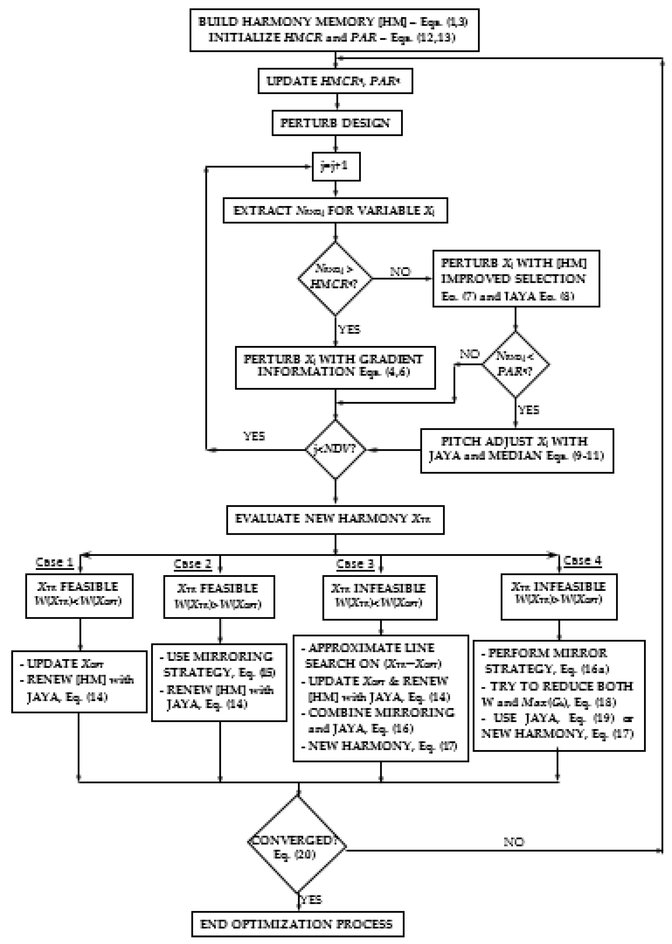
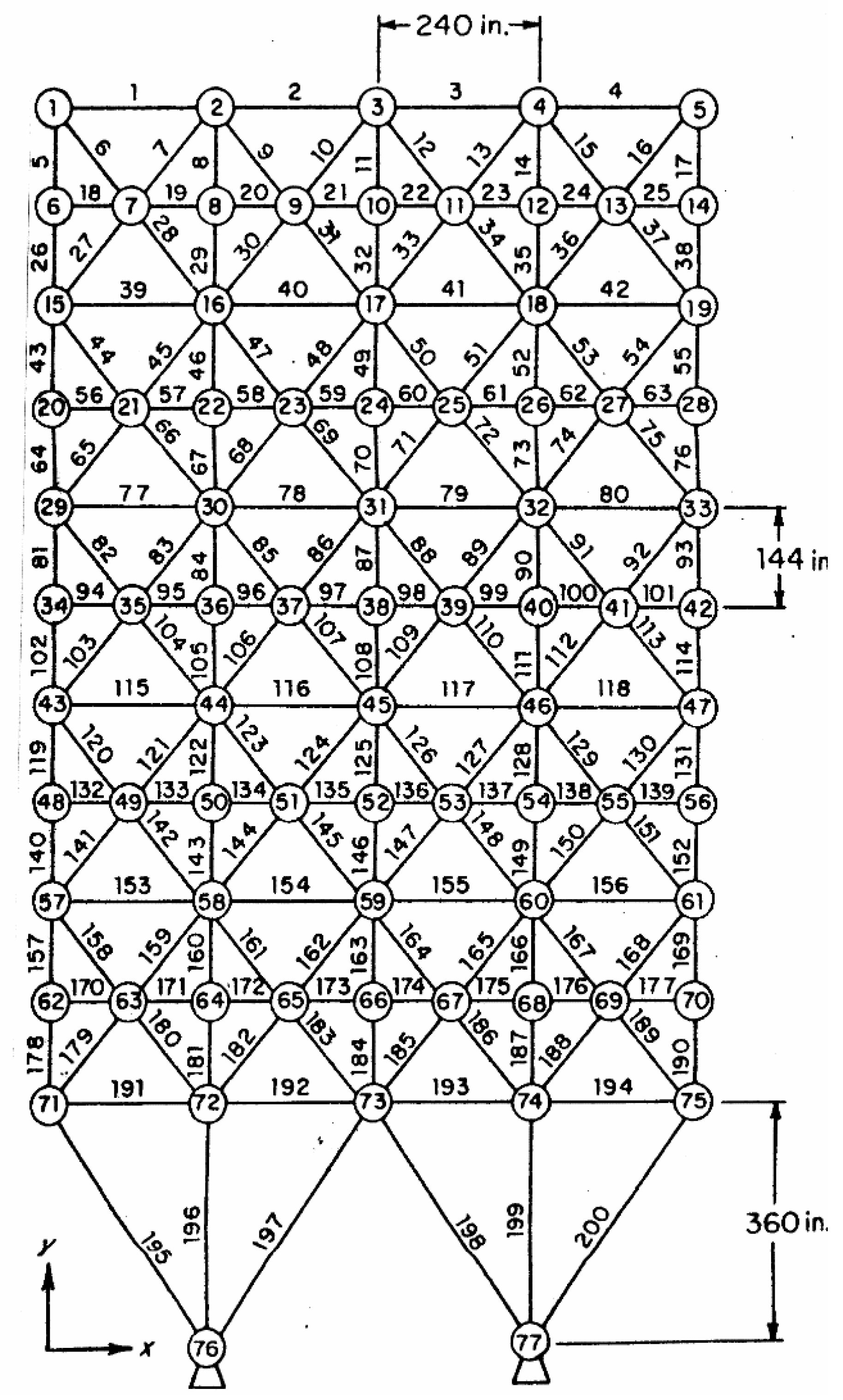
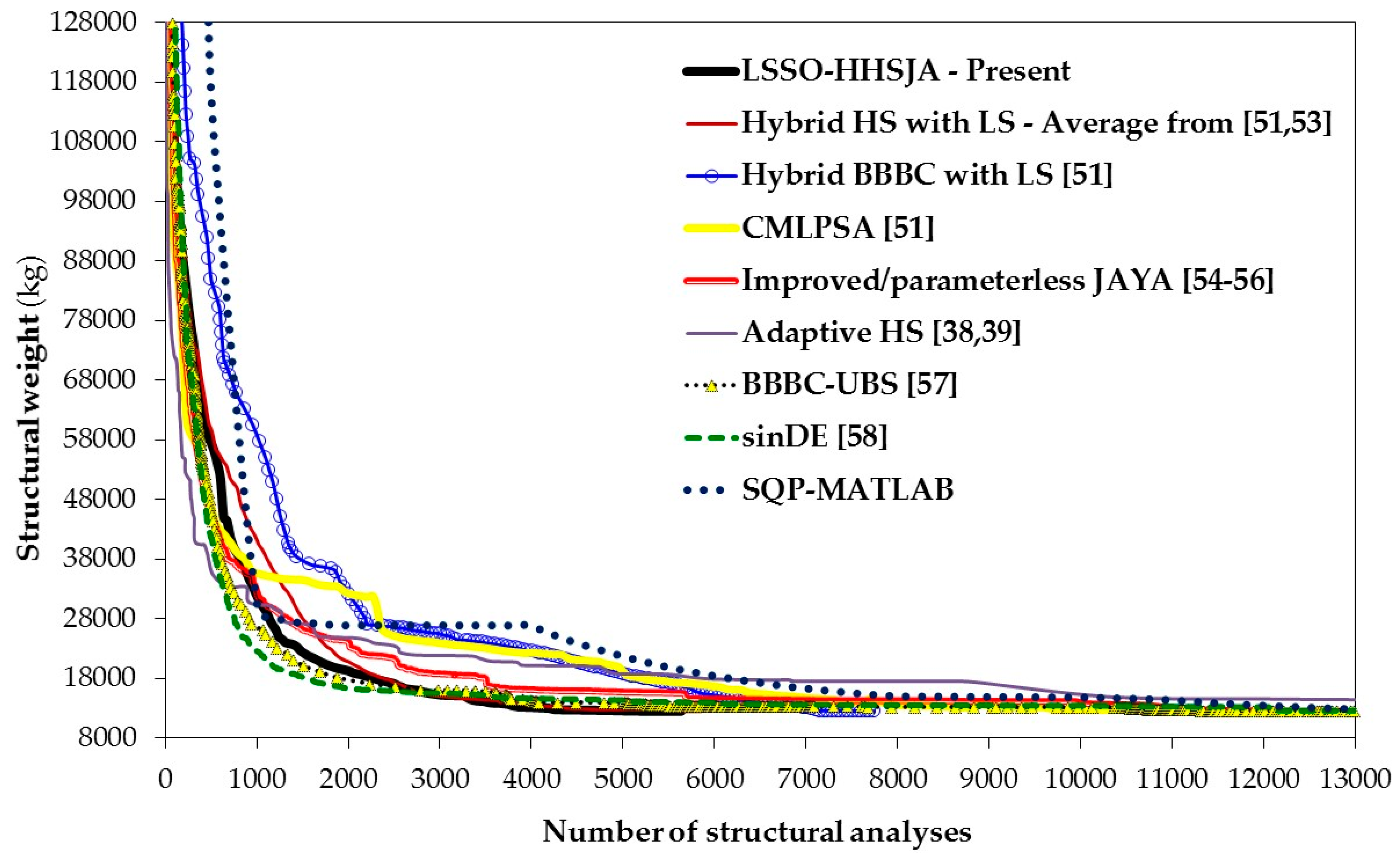
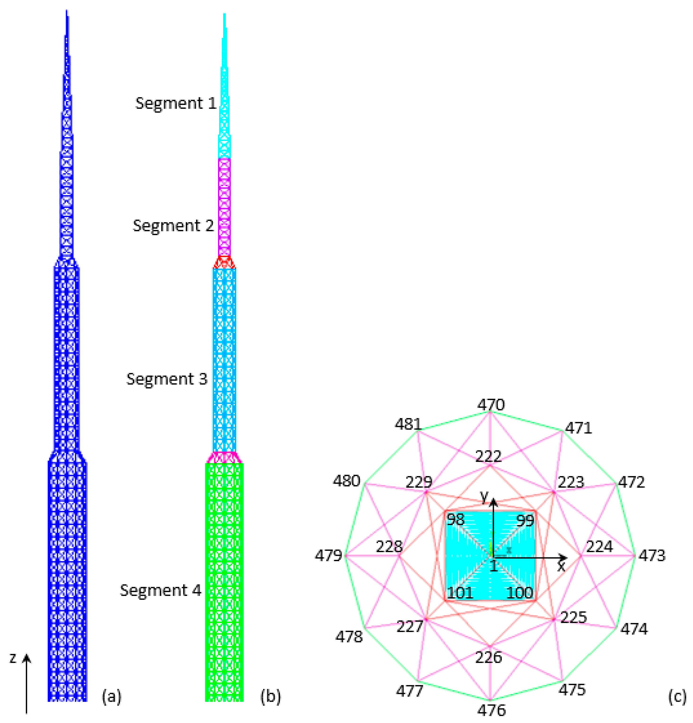
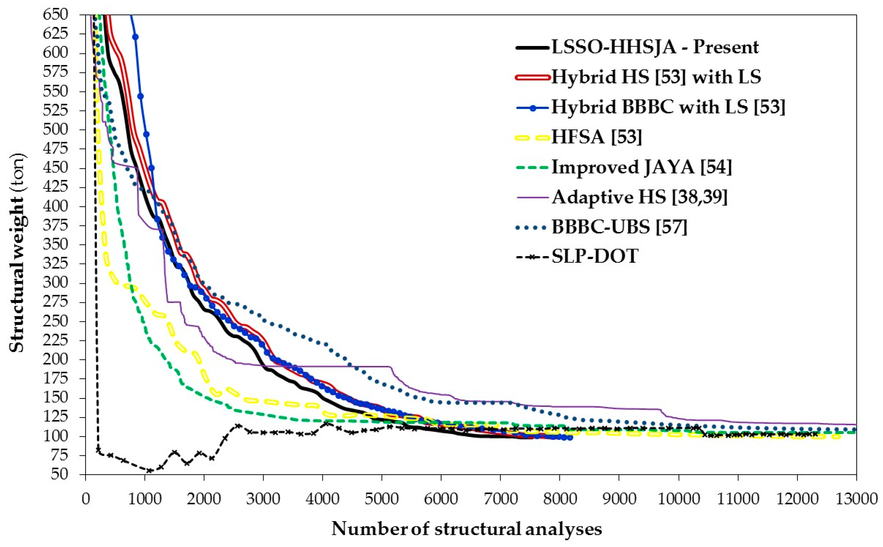
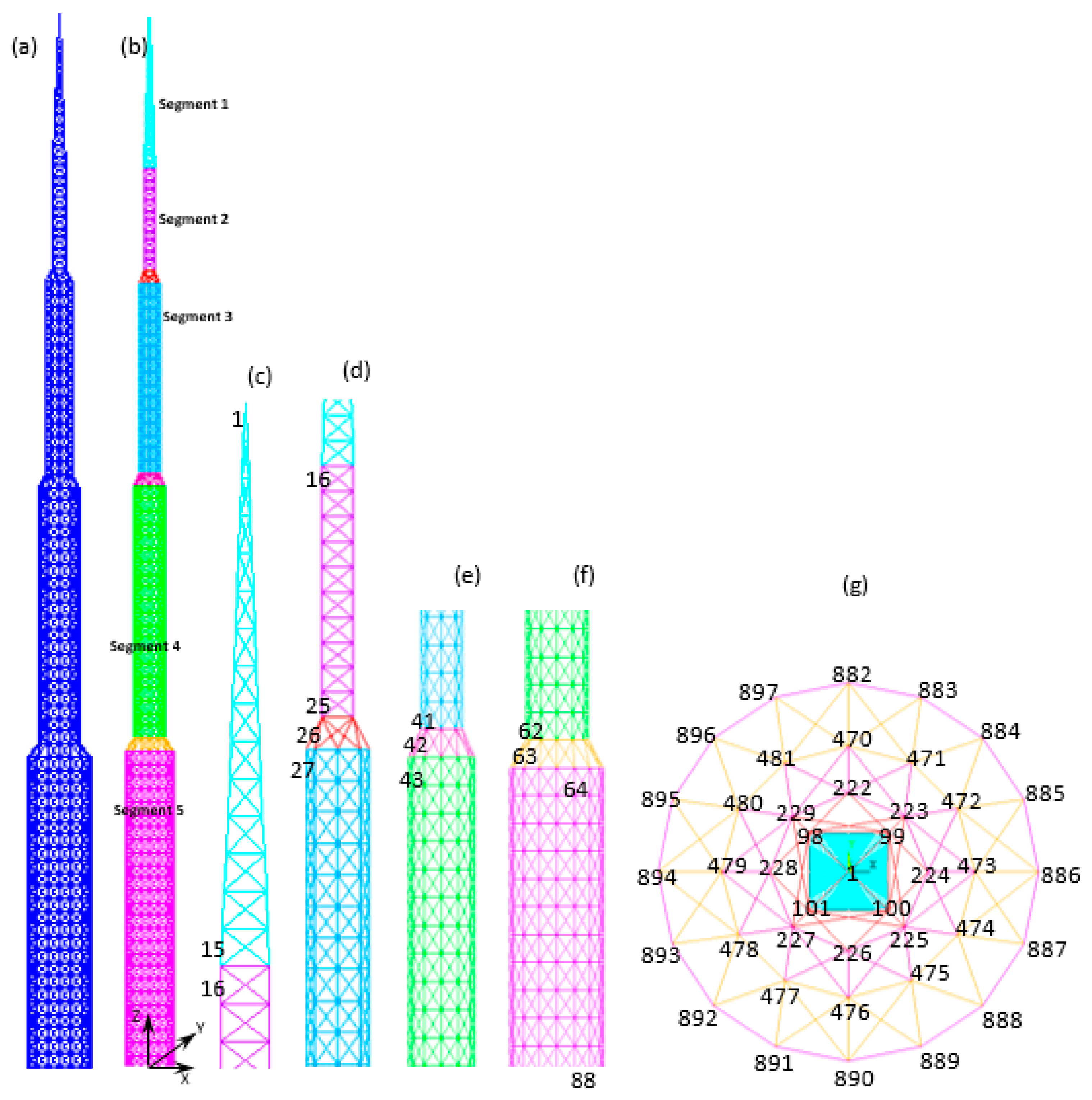
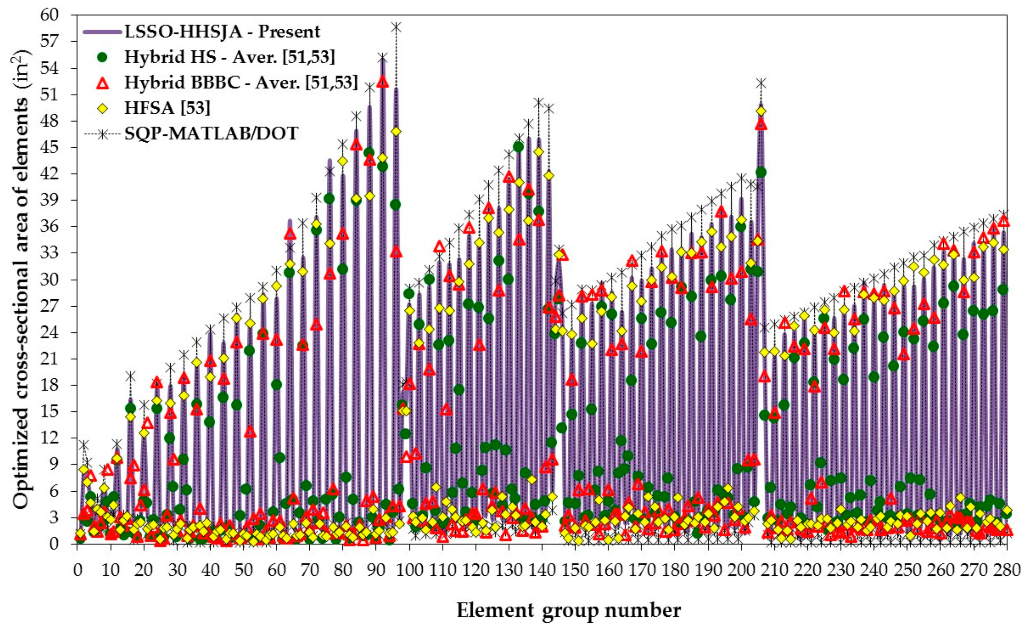
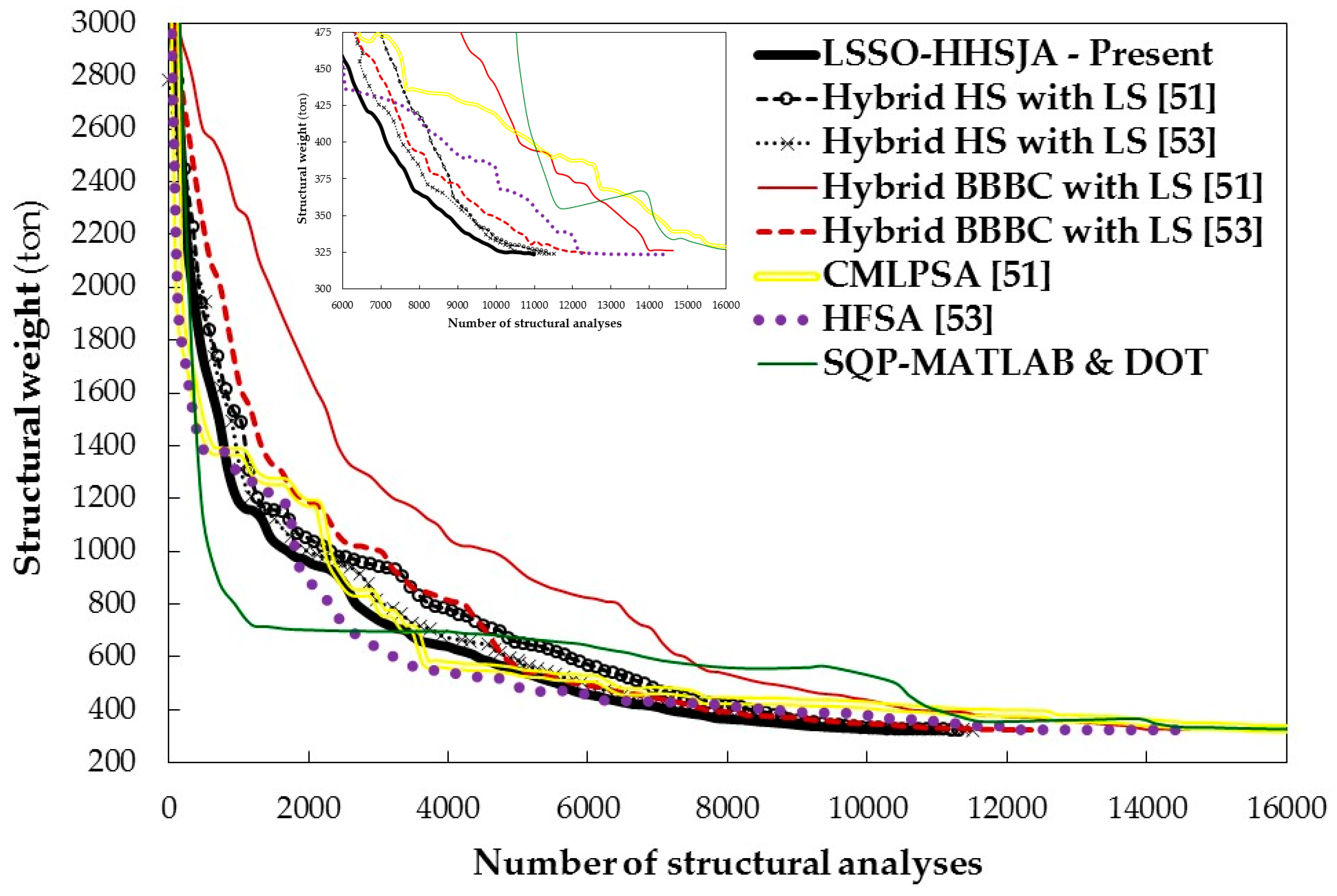
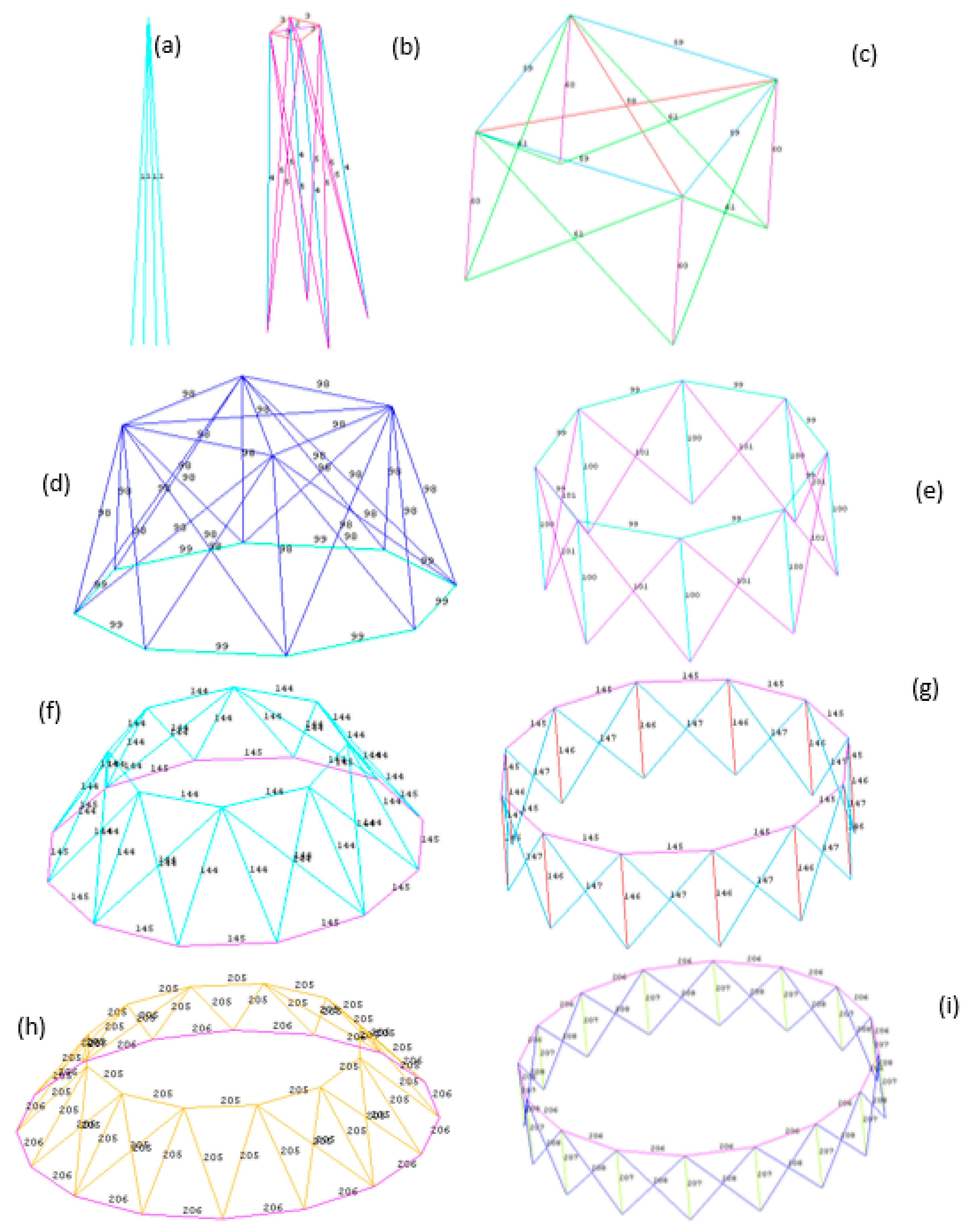
Table A1.
Element grouping for the two space towers optimized in this study. Group element numbers are indicated between parentheses. Elements shared by the two towers are typed in bold.
Table A1.
Element grouping for the two space towers optimized in this study. Group element numbers are indicated between parentheses. Elements shared by the two towers are typed in bold.
| (1) 1–4 | (41) 177–184 | (81) 357–364 | (121) 695–702 | (161) 1231–1242 | (201) 1867–1890 | (241) 2723–2754 |
| (2) 5–6 | (42) 185–186 | (82) 365–366 | (122) 703–718 | (162) 1243–1266 | (202) 1891–1902 | (242) 2755–2770 |
| (3) 7–10 | (43) 187–190 | (83) 367–370 | (123) 719–726 | (163) 1267–1278 | (203) 1903–1914 | (243) 2771–2786 |
| (4) 11–14 | (44) 191–194 | (84) 371–374 | (124) 727–734 | (164) 1279–1290 | (204) 1915–1938 | (244) 2787–2818 |
| (5) 15–22 | (45) 195–202 | (85) 375–382 | (125) 735–750 | (165) 1291–1314 | (205) 1939–1986 | (245) 2819–2834 |
| (6) 23–24 | (46) 203–204 | (86) 383–384 | (126) 751–758 | (166) 1315–1326 | (206) 1987–2002 | (246) 2835–2850 |
| (7) 25–28 | (47) 205–208 | (87) 385–388 | (127) 759–766 | (167) 1327–1338 | (207) 2003–2018 | (247) 2851–2882 |
| (8) 29–32 | (48) 209–212 | (88) 389–392 | (128) 767–782 | (168) 1339–1362 | (208) 2019–2050 | (248) 2883–2898 |
| (9) 33–40 | (49) 213–220 | (89) 393–400 | (129) 783–790 | (169) 1363–1374 | (209) 2051–2066 | (249) 2899–2914 |
| (10) 41–42 | (50) 221–222 | (90) 401–402 | (130) 791–798 | (170) 1375–1386 | (210) 2067–2082 | (250) 2915–2946 |
| (11) 43–46 | (51) 223–226 | (91) 403–406 | (131) 799–814 | (171) 1387–1410 | (211) 2083–2114 | (251) 2947–2962 |
| (12) 47–50 | (52) 227–230 | (92) 407–410 | (132) 815–822 | (172) 1411–1422 | (212) 2115–2130 | (252) 2963–2978 |
| (13) 51–58 | (53) 231–238 | (93) 411–418 | (133) 823–830 | (173) 1423–1434 | (213) 2131–2146 | (253) 2979–3010 |
| (14) 59–60 | (54) 239–240 | (94) 419–420 | (134) 831–846 | (174) 1435–1458 | (214) 2147–2178 | (254) 3011–3026 |
| (15) 61–64 | (55) 241–244 | (95) 421–424 | (135) 847–854 | (175) 1459–1470 | (215) 2179–2194 | (255) 3027–3042 |
| (16) 65–68 | (56) 245–248 | (96) 425–428 | (136) 855–862 | (176) 1471–1482 | (216) 2195–2210 | (256) 3043–3074 |
| (17) 69–76 | (57) 249–256 | (97) 429–436 | (137) 863–878 | (177) 1483–1506 | (217) 2211–2242 | (257) 3075–3090 |
| (18) 77–78 | (58) 257–258 | (98) 437–462 | (138) 879–886 | (178) 1507–1518 | (218) 2243–2258 | (258) 3091–3106 |
| (19) 79–82 | (59) 259–262 | (99) 463–470 | (139) 887–894 | (179) 1519–1530 | (219) 2259–2274 | (259) 3107–3138 |
| (20) 83–86 | (60) 263–266 | (100) 471–478 | (140) 895–910 | (180) 1531–1554 | (220) 2275–2306 | (260) 3139–3154 |
| (21) 87–94 | (61) 267–274 | (101) 479–494 | (141) 911–918 | (181) 1555–1566 | (221) 2307–2322 | (261) 3155–3170 |
| (22) 95–96 | (62) 275–276 | (102) 495–502 | (142) 919–926 | (182) 1567–1578 | (222) 2323–2338 | (262) 3171–3202 |
| (23) 97–100 | (63) 277–280 | (103) 503–510 | (143) 927–942 | (183) 1579–1602 | (223) 2339–2370 | (263) 3203–3218 |
| (24) 101–104 | (64) 281–284 | (104) 511–526 | (144) 943–978 | (184) 1603–1614 | (224) 2371–2386 | (264) 3219–3234 |
| (25) 105–112 | (65) 285–292 | (105) 527–534 | (145) 979–990 | (185) 1615–1626 | (225) 2387–2402 | (265) 3235–3266 |
| (26) 113–114 | (66) 293–294 | (106) 535–542 | (146) 991–1002 | (186) 1627–1650 | (226) 2403–2434 | (266) 3267–3282 |
| (27) 115–118 | (67) 295–298 | (107) 543–558 | (147) 1003–1026 | (187) 1651–1662 | (227) 2435–2450 | (267) 3283–3298 |
| (28) 119–122 | (68) 299–302 | (108) 559–566 | (148) 1027–1038 | (188) 1663–1674 | (228) 2451–2466 | (268) 3299–3330 |
| (29) 123–130 | (69) 303–310 | (109) 567–574 | (149) 1039–1050 | (189) 1675–1698 | (229) 2467–2498 | (269) 3331–3346 |
| (30) 131–132 | (70) 311–312 | (110) 575–590 | (150) 1051–1074 | (190) 1699–1710 | (230) 2499–2514 | (270) 3347–3362 |
| (31) 133–136 | (71) 313–316 | (111) 591–598 | (151) 1075–1086 | (191) 1711–1722 | (231) 2515–2530 | (271) 3363–3394 |
| (32) 137–140 | (72) 317–320 | (112) 599–606 | (152) 1087–1098 | (192) 1723–1746 | (232) 2531–2562 | (272) 3395–3410 |
| (33) 141–148 | (73) 321–328 | (113) 607–622 | (153) 1099–1122 | (193) 1747–1758 | (233) 2563–2578 | (273) 3411–3426 |
| (34) 149–150 | (74) 329–330 | (114) 623–630 | (154) 1123–1134 | (194) 1759–1770 | (234) 2579–2594 | (274) 3427–3458 |
| (35) 151–154 | (75) 331–334 | (115) 631–638 | (155) 1135–1146 | (195) 1771–1794 | (235) 2595–2626 | (275) 3459–3474 |
| (36) 155–158 | (76) 335–338 | (116) 639–654 | (156) 1147–1170 | (196) 1795–1806 | (236) 2627–2642 | (276) 3475–3490 |
| (37) 159–166 | (77) 339–346 | (117) 655–662 | (157) 1171–1182 | (197) 1807–1818 | (237) 2643–2658 | (277) 3491–3522 |
| (38) 167–168 | (78) 347–348 | (118) 663–670 | (158) 1183–1194 | (198) 1819–1842 | (238) 2659–2690 | (278) 3523–3538 |
| (39) 169–172 | (79) 349–352 | (119) 671–686 | (159) 1195–1218 | (199) 1843–1854 | (239) 2691–2706 | (279) 3539–3554 |
| (40) 173–176 | (80) 353–356 | (120) 687–694 | (160) 1219–1230 | (200) 1855–1866 | (240) 2707–2722 | (280) 3555–3586 |
Figure A1.
Details of element group numbering for the spatial 3586-bar truss tower: (a) Top-level storey of the square-based pyramid segment; (b) Second storey from the top of the tower; (c) Top-level storey of the square-based prismatic segment; (d) Transition from the bottom level-storey of the square-based prismatic segment to the top-level storey of the octagon-based prismatic segment; (e) Top-level storey of the octagon-based prismatic segment; (f) Transition from the bottom-level storey of the octagon-based prismatic segment to the top-level storey of the dodecagon-based prismatic segment; (g) Top-level storey of the dodecagon-based prismatic segment; (h) Transition from the bottom-level storey of the dodecagon-based prismatic segment to the top-level storey of the hexadecagon-based prismatic segment; (i) Top-level storey of the hexadecagon-based prismatic segment.

References
- Goldberg, D.E. Genetic Algorithms in Search, Operation and Machine Learning; Addison-Wesley: Boston, MA, USA, 1989. [Google Scholar]
- Storn, R.; Price, K. Differential Evolution—A Simple and Efficient Adaptive Scheme for Global Optimization over Continuous Spaces; Technical Report No. TR-95-012; International Computer Science Institute: Berkley, CA, USA, 1995. [Google Scholar]
- Van Laarhoven, P.J.M.; Aarts, E.H.L. Simulated Annealing: Theory and Applications; Kluwer Academic Publishers: Dordrecht, The Netherlands, 1987. [Google Scholar]
- Clerc, M. Particle Swarm Optimization; ISTE Publishing Company: London, UK, 2006. [Google Scholar]
- Dorigo, M.; Stutzle, T. Ant Colony Optimization; MIT Press: Cambridge, MA, USA, 2004. [Google Scholar]
- Gandomi, A.H.; Yang, X.S.; Alavi, A.H. Mixed variable structural optimization using firefly algorithm. Comput. Struct. 2011, 89, 2325–2336. [Google Scholar] [CrossRef]
- Gandomi, A.H.; Yang, X.S.; Alavi, A.H. Cuckoo search algorithm: A metaheuristic approach to solve structural optimization problems. Eng. Comput. 2013, 29, 17–35. [Google Scholar] [CrossRef]
- Mirjalili, S. The ant lion optimizer. Adv. Eng. Softw. 2015, 83, 80–98. [Google Scholar] [CrossRef]
- Glover, F.; Laguna, M. Tabu Search; Kluwer Academic Publishers: Boston, MA, USA, 1997. [Google Scholar]
- Geem, Z.W.; Kim, J.H.; Loganathan, G. A new heuristic optimization algorithm: Harmony search. Simulation 2001, 76, 60–68. [Google Scholar] [CrossRef]
- Rao, R.V.; Savsani, V.J.; Vakharia, D.P. Teaching–learning-based optimization: A novel method for constrained mechanical design optimization problems. Comput. Aided Des. 2011, 43, 303–315. [Google Scholar] [CrossRef]
- Rao, R.V. Jaya: A simple and new optimization algorithm for solving constrained and unconstrained optimization problems. Int. J. Ind. Eng. Comp. 2016, 7, 19–34. [Google Scholar]
- Erol, O.K.; Eksin, I. A new optimization method: Big bang-big crunch. Adv. Eng. Softw. 2006, 37, 106–111. [Google Scholar] [CrossRef]
- Kaveh, A.; Talatahari, S. A novel heuristic optimization method: Charged system search. Acta Mech. 2010, 213, 267–289. [Google Scholar] [CrossRef]
- Kaveh, A.; Khayat Azad, M. A new meta-heuristic method: Ray optimization. Comput. Struct. 2012, 112–113, 283–294. [Google Scholar] [CrossRef]
- Kaveh, A.; Mahdavi, V.R. Colliding bodies optimization: A novel meta-heuristic method. Comput. Struct. 2014, 139, 18–27. [Google Scholar] [CrossRef]
- Kaveh, A.; Bakhshpoori, T. A new metaheuristic for continuous structural optimization: Water evaporation optimization. Struct. Multidiscip. Optim. 2016, 54, 23–43. [Google Scholar] [CrossRef]
- Kaveh, A.; Zolghadr, A. Cyclical parthenogenesis algorithm for guided modal strain energy based structural damage detection. Appl. Soft Comput. 2017, 57, 250–264. [Google Scholar] [CrossRef]
- Pierezan, J.; Coelho, L.S. Coyote optimization algorithm: A new metaheuristic for global optimization problems. In Proceedings of the IEEE World Conference on Computational Intelligence, Congress on Evolutionary Computation, Rio de Janeiro, Brazil, 8–13 July 2018; pp. 2633–2640. [Google Scholar]
- Lamberti, L.; Pappalettere, C. Metaheuristic design optimization of skeletal structures: A review. Comput. Technol. Rev. 2011, 4, 1–32. [Google Scholar] [CrossRef]
- Saka, M.P.; Dogan, E. Recent developments in metaheuristic algorithms: A review. Comput. Technol. Rev. 2012, 5, 31–78. [Google Scholar] [CrossRef]
- Kaveh, A. Advances in Metaheuristic Algorithms for Optimal Design of Structures; Springer International Publishing: Cham, Switzerland, 2014. [Google Scholar]
- Kaveh, A. Applications of Metaheuristic Optimization Algorithms in Civil Engineering; Springer International Publishing: Cham, Switzerland, 2017. [Google Scholar]
- Kaveh, A.; Ilchi Ghazaan, M. Meta-Heuristic Algorithms for Optimal Design of Real-Size Structures; Springer International Publishing: Cham, Switzerland, 2018. [Google Scholar]
- Wolpert, D.H.; Macready, W.G. No Free Lunch Theorems for optimization. IEEE Trans. Evol. Comput. 1997, 1, 67–82. [Google Scholar] [CrossRef] [Green Version]
- Ho, Y.C.; Pepyne, D.L. Simple explanation of the No-Free-Lunch Theorem and its implications. J. Optim. Theory Appl. 2002, 115, 549–570. [Google Scholar] [CrossRef]
- Yang, X.-S. Harmony search as a metaheuristic algorithm. In Music-Inspired Harmony Search Algorithm: Theory and Applications; Geem, Z.W., Ed.; Springer: Berlin/Heidelberg, Germany, 2009; pp. 1–14. [Google Scholar]
- Haftka, R.T.; Gurdal, Z. Elements of Structural Optimization, 3rd ed.; Kluwer Academic Publishers: Dordrecht, The Netherlands, 1992. [Google Scholar]
- Vanderplaats, G.N. Numerical Optimization Techniques for Engineering Design; VR&D Inc.: Colorado Springs, CO, USA, 1998. [Google Scholar]
- Arora, J.S. Introduction to Optimum Design; McGraw-Hill Book Company: New York, NY, USA, 1989. [Google Scholar]
- Lee, K.S.; Geem, Z.W. A new structural optimization method based on the harmony search algorithm. Comput. Struct. 2004, 82, 781–798. [Google Scholar] [CrossRef]
- Lee, K.S.; Geem, Z.W. A new meta-heuristic algorithm for continuous engineering optimization: Harmony search theory and practice. Comput. Methods Appl. Mech. Eng. 2005, 194, 3902–3933. [Google Scholar] [CrossRef]
- Saka, M.P. Optimum design of steel sway frames to BS5950 using harmony search algorithm. J. Constr. Steel Res. 2009, 65, 36–43. [Google Scholar] [CrossRef]
- Maheri, M.R.; Narimani, M.N. An enhanced harmony search algorithm for optimum design of side sway steel frames. Comput. Struct. 2014, 136, 78–89. [Google Scholar] [CrossRef]
- Murren, P.; Khandelwal, K. Design-driven harmony search (DDHS) in steel frame optimization. Eng. Struct. 2014, 59, 798–808. [Google Scholar] [CrossRef]
- Mahdavi, M.; Fesanghary, M.; Damangir, E. An improved harmony search algorithm for solving optimization problems. Appl. Math. Comput. 2007, 188, 1567–1579. [Google Scholar] [CrossRef]
- Carbas, S.; Saka, M.P. Optimum topology design of various geometrically nonlinear latticed domes using improved harmony search method. Struct. Multidiscip. Optim. 2012, 45, 377–399. [Google Scholar] [CrossRef]
- Hasancebi, O.; Erdal, F.; Saka, M.P. Adaptive harmony search method for structural optimization. ASCE J. Struct. Eng. 2010, 136, 419–431. [Google Scholar] [CrossRef]
- Degertekin, S.O. Improved harmony search algorithms for sizing optimization of truss structures. Comput. Struct. 2012, 92–93, 229–241. [Google Scholar] [CrossRef]
- Kaveh, A.; Naiemi, M. Sizing optimization of skeletal structures with a multi-adaptive Harmony Search algorithm. Sci. Iran. Trans. Civil Eng. 2015, 22, 345–366. [Google Scholar]
- Geem, Z.W.; Sim, K.B. Parameter-setting-free harmony search algorithm. Appl. Math. Comput. 2010, 217, 3881–3889. [Google Scholar] [CrossRef]
- Turky, A.M.; Abdullah, S. A multi-population harmony search algorithm with external archive for dynamic optimization problems. Inform. Sci. 2014, 272, 84–95. [Google Scholar] [CrossRef]
- Kaveh, A.; Ahangaran, M. Discrete cost optimization of composite floor system using social harmony search model. Appl. Soft Comput. 2012, 12, 372–381. [Google Scholar] [CrossRef]
- Cheng, M.Y.; Prayogo, D.; Wu, Y.W.; Lukito, M.M. A Hybrid Harmony Search algorithm for discrete sizing optimization of truss structure. Auto. Constr. 2016, 69, 21–33. [Google Scholar] [CrossRef]
- Kaveh, A.; Talatahari, S. A particle swarm ant colony optimization for truss structures with discrete variables. J. Constr. Steel Res. 2009, 65, 1558–1568. [Google Scholar] [CrossRef]
- Kaveh, A.; Talatahari, S. Particle swarm optimizer, ant colony strategy and harmony search scheme hybridized for optimization of truss structures. Comput. Struct. 2009, 87, 267–283. [Google Scholar] [CrossRef]
- Omran, M.G.H.; Mahdavi, M. Global best harmony search. Appl. Math. Comput. 2008, 198, 643–656. [Google Scholar] [CrossRef]
- Al-Betar, M.A.; Abu Doush, I.; Khader, A.T.; Awadallah, M.A. Novel selection schemes for harmony search. Appl. Math. Comput. 2012, 218, 6095–6117. [Google Scholar] [CrossRef]
- Fesanghary, M.; Mahdavi, M.; Minary-Jolandan, M.; Alizadeh, Y. Hybridizing harmony search algorithm with sequential quadratic programming for engineering optimization problems. Comput. Methods Appl. Mech. Eng. 2008, 197, 3080–3091. [Google Scholar] [CrossRef]
- Lamberti, L.; Pappalettere, C. An improved harmony-search algorithm for truss structure optimization. In Proceedings of the Twelfth International Conference on Civil, Structural and Environmental Engineering Computing, Funchal, Portugal, 1–4 September 2009; Topping, B.H.V., Costa Neves, L.F., Barros, R.C., Eds.; [Google Scholar]
- Lamberti, L.; Pappalettere, C. Truss weight minimization using hybrid Harmony Search and Big Bang-Big Crunch algorithms. In Metaheuristic Applications in Structures and Infrastructures; Gandomi, A.H., Yang, X.S., Talatahari, S., Alavi, A.H., Eds.; Elsevier: Waltham, MA, USA, 2013; pp. 207–240. [Google Scholar]
- Degertekin, S.O.; Lamberti, L. Comparison of hybrid metaheuristic algorithms for truss weight optimization. In Proceedings of the Third International Conference on Soft Computing Technology in Civil, Structural and Environmental Engineering, Cagliari, Italy, 3–6 September 2013; Tsompanakis, Y., Ed.; [Google Scholar]
- Ficarella, E.; Lamberti, L.; Degertekin, S.O. Comparison of three novel hybrid metaheuristic algorithms for structural optimization problems. Comput. Struct. 2021, 244, 106395. [Google Scholar] [CrossRef]
- Degertekin, S.O.; Lamberti, L.; Ugur, I.B. Sizing, layout and topology design optimization of truss structures using the Jaya algorithm. Appl. Soft Comput. 2018, 70, 903–928. [Google Scholar] [CrossRef]
- Degertekin, S.O.; Lamberti, L.; Ugur, I.B. Discrete sizing/layout/topology optimization of truss structures with an advanced Jaya algorithm. Appl. Soft Comput. 2019, 79, 363–390. [Google Scholar] [CrossRef]
- Degertekin, S.O.; Yalcin Bayar, G.; Lamberti, L. Parameter free Jaya algorithm for truss sizing-layout optimization under natural frequency constraints. Comput. Struct. 2021, 245, 106461. [Google Scholar] [CrossRef]
- Kazemzadeh Azad, S.; Hasancebi, O.; Kazemzadeh Azad, S.; Erol, O.K. Upper bound strategy in optimum design of truss structures: A big bang-big crunch algorithm based application. Adv. Struct. Eng. 2013, 16, 1035–1046. [Google Scholar] [CrossRef]
- Draa, A.; Bouzoubia, S.; Boukhalfa, I. A sinusoidal differential evolution algorithm for numerical optimization. Appl. Soft Comput. 2015, 27, 99–126. [Google Scholar] [CrossRef]
- The MathWorks. MATLAB® Release 2018b; The MathWorks: Austin, TX, USA, 2018. [Google Scholar]
- Vanderplaats, G.N. DOTs Users Manual, Version 4.20; VR&D Inc.: Colorado Springs, CO, USA, 1995. [Google Scholar]
Figure 1.
Flow chart of the hybrid LSSO-HHSJA algorithm developed in this research.

Figure 2.
Schematic of the planar 200-bar truss structure.

Figure 3.
Convergence curves obtained for the 200-bar truss design example.

Figure 4.
Schematic of the spatial 1938-bar tower: (a) Assembly view; (b) Color view of the four segments and two junction modules included in the structure; (c) Layout view indicating key-nodes.
Figure 4.
Schematic of the spatial 1938-bar tower: (a) Assembly view; (b) Color view of the four segments and two junction modules included in the structure; (c) Layout view indicating key-nodes.

Figure 5.
Convergence curves obtained for the 1938-bar tower design example.

Figure 6.
Schematic of the spatial 3586-bar tower (representative story and junction numbers also are shown): (a) Assembly view; (b) Color view of the five segments and three junction modules included in the structure; (c) Transition from the top of the tower to segment 1 (top of the structure); (d,e) Transitions between segments 2 and 3, and between segments 3 and 4 (center of the structure); (f) Transition between segments 4 and 5 (bottom of the structure); (g) Layout view indicating key-nodes.

Figure 7.
Optimized cross-sectional areas of the 3586-bar tower.

Figure 8.
Convergence curves obtained for the 3586-bar tower design example.

Table 1.
Sensitivity of LSSO-HHSJA and other hybrid HS variants’ convergence behavior to population size for the 200-bar truss problem.
Table 1.
Sensitivity of LSSO-HHSJA and other hybrid HS variants’ convergence behavior to population size for the 200-bar truss problem.
| NPOP | Structural Weight (kg) | Structural Analyses | Constraint Tolerance (%) |
|---|---|---|---|
| 20 | 12,483.673 | 5562 | Feasible |
| 12,490.377 * | 5668 * | 0.00735 * | |
| 12,489.460 ♦ | 5716 ♦ | 0.003451 ♦ | |
| 50 | 12,483.563 | 5734 | Feasible |
| 12,490.482 * | 6604 * | 0.00750 * | |
| 12,489.457 ♦ | 6040 ♦ | 0.003250 ♦ | |
| 100 | 12,484.135 | 6096 | Feasible |
| 12,490.542 * | 6360 * | 0.00750 * | |
| 12,489.778 ♦ | 5621 ♦ | 0.002802 ♦ | |
| 200 | 12,483.982 | 5436 | Feasible |
| 12,490.332 * | 5679 * | 0.00730 * | |
| 12,489.700 ♦ | 5831 ♦ | 0.003168 ♦ | |
| 500 | 12,483.339 | 5637 | Feasible |
| 12,490.414* | 5940 * | 0.00643 * | |
| 12,489.619 ♦ | 6372 ♦ | 0.003524 ♦ | |
| 1000 | 12,484.054 | 6373 | Feasible |
| 12,490.427* | 5938 * | 0.00560 * | |
| 12,489.564 ♦ | 6217 ♦ | 0.003329 ♦ |
Table 2.
Optimization results obtained for the 200-bar truss design example.
| Optimized Weight (kg) | Number of Structural Analyses | Constraint Violation (%) | |
|---|---|---|---|
| LSSO-HHSJA Present | Best: 12,483.339 | Best: 5637 | |
| Worst: 12,484.135 | Fastest: 5436 | Feasible | |
| Mean: 12,483.791 | Slowest: 6373 | ||
| STD: 0.3144 | Mean/STD: 5806 ± 357 | ||
| Hybrid HS with LS [51] | Best: 12,490.332 | Best: 5679 | Best: 0.00730 |
| Worst: 12,490.542 | Fastest: 5668 | Worst: 0.00750 | |
| Mean: 12,490.430 | Slowest: 6604 | Mean: 0.00695 | |
| STD: 0.07470 | Mean/STD: 6031 ± 377 | STD: 0.000772 | |
| Hybrid HS with LS [53] | Best: 12,489.457 | Best: 6040 | Best: 0.003250 |
| Worst: 12,489.778 | Fastest: 5621 | Worst: 0.002802 | |
| Mean: 12,489.596 | Slowest: 6372 | Mean: 0.003254 | |
| STD: 0.1291 | Mean/STD: 5966 ± 324 | STD: 0.0002565 | |
| Hybrid BBBC with LS [51] | Best: 12,490.439 | Best: 7745 | Best: 0.00559 |
| Worst: 12,490.932 | Fastest: 1924 | Worst: 0.00625 | |
| Mean: 12,490.680 | Slowest: 9460 | Mean: 0.00626 | |
| STD: 0.1773 | Mean/STD: 5652 ± 2912 | STD: 0.000347 | |
| CMLPSA [51] | Best: 12,492.888 | Best: 11,726 | |
| Worst: 12,493.290 | Fastest: 10,338 | Feasible | |
| Mean: 12,493.081 | Slowest: 12,118 | ||
| STD: 0.2014 | Mean/STD: 11,394 ± 935 | ||
| Improved/parameterless JAYA [54,55,56] | Best: 12,490.603 | Best: 12,869 | Best: 0.03490 |
| Worst: 12,502.175 | Fastest: 12,316 | Worst: Feasible | |
| Mean: 12,494.460 | Slowest: 14,326 | Mean: 0.01888 | |
| STD: 3.056 | Mean/STD: 12,818 ± 601 | STD: 0.01644 | |
| AHS [38] | Best: 12,497.475 | Best: 16,981 | Best: 0.1570 |
| Worst: 12,777.339 | Fastest: 15,063 | Worst: Feasible | |
| Mean: 12,567.441 | Slowest: 21,412 | Mean: 0.08363 | |
| STD: 174.716 | Mean/STD: 17,130 ± 2996 | STD: 0.06836 | |
| SAHS [39] | Best: 12,495.939 | Best: 15,812 | Best: 0.1824 |
| Worst: 12,669.384 | Fastest: 13,384 | Worst: Feasible | |
| Mean: 12,553.754 | Slowest: 17,464 | Mean: 0.09718 | |
| STD: 144.817 | Mean/STD: 15,618 ± 1681 | STD: 0.07942 | |
| BBBC-UBS [57] | Best: 12,490.035 | Best: 15,250 | Best: 0.05540 |
| Worst: 12,502.346 | Fastest: 13,865 | Worst: Feasible | |
| Mean: 12,497.562 | Slowest: 16,198 | Mean: 0.03048 | |
| STD: 4.170 | Mean/STD: 14,795 ± 1141 | STD: 0.02837 | |
| sinDE [58] | Best: 12,502.536 | Best: 21,653 | Best: 0.05880 |
| Worst: 12,541.640 | Fastest: 17,124 | Worst: Feasible | |
| Mean: 12,520.999 | Slowest: 22,635 | Mean: 0.03030 | |
| STD: 16.369 | Mean/STD: 20,766 ± 2472 | STD: 0.03017 | |
| SQP-MATLAB | Best: 12,491.400 | Best: 28,198 | Best: 0.05131 |
| Worst: 12,503.300 | Fastest: 24,619 | Worst: Feasible | |
| Mean: 12,498.034 | Slowest: 38,410 | Mean: 0.03298 | |
| STD: 5.661 | Mean/STD: 30,990 ± 5957 | STD: 0.03969 |
Table 3.
Loading conditions acting on the 1938-bar tower.
| Loading Condition 1 | |
| X | None |
| Y | None |
| Z | −13.5 kN @ nodes 1 through 61 (the “–“ sign indicates that concentrated forces act in the negative Z-direction); −27 kN @ nodes 62 through 101; −40.5 kN @ nodes 102 through 229; −54 kN @ nodes 230 through 469. |
| Loading condition 2 | |
| X | +6.672 kN @ nodes 2, 5, 6, 9, 10, 13, 14, 17, 18, 21, 22, 25, 26, 29, 30, 33, 34, 37, 38, 41, 42, 45, 46, 49, 50, 53, 54, 57, 58, 61, 62, 65, 66, 69, 70, 81, 82, 85, 86, 89, 90, 93, 94, 97, 98, 101, 108, 116, 124, 132, 140, 148, 156, 164, 172, 180, 188, 196, 204, 220, 228, 239, 251, 263, 275, 287, 299, 311, 323, 335, 347, 359, 371, 383, 395, 407, 419, 431, 443, 455, 467; −4.448 kN @ nodes 3, 4, 7, 8, 11, 12, 15, 16, 19, 20, 23, 24, 27, 28, 31, 32, 35, 36, 39, 40, 43, 44, 47, 48, 51, 52, 55, 56, 59,60, 63, 64, 67, 68, 71, 72, 75, 76, 79, 80, 83, 84, 87, 88, 91, 92, 95, 96, 99, 100, 104, 112, 120, 128, 136, 144, 152, 160, 168, 176, 184, 192, 200, 208, 216, 224, 233, 245, 257, 269, 281, 293, 305, 317, 329, 341, 353, 365, 377, 389, 401, 413, 425, 437, 449, 461 (the “–“ sign indicates that concentrated forces act in the negative X-direction). |
| Y | None |
| Z | None |
| Loading condition 3 | |
| X | None |
| Y | −4.448 kN @ nodes 2, 3, 6, 7, 10, 11, 14, 15, 18, 19, 22, 23, 26, 27, 30, 31, 34, 35, 38, 39, 42, 43, 46, 47, 50, 51, 54, 55, 58, 59, 62, 63, 66, 67, 70, 71, 74, 75, 78, 79, 82, 83, 86, 87, 90, 91, 94, 95, 98, 99, 102, 110, 118, 126, 134, 142, 150, 158, 166, 174, 182, 190, 198, 206, 214, 222, 230, 242, 266, 278, 290, 302, 314, 326, 338, 350, 362, 374, 386, 398, 410, 422, 434, 446, 458 (the “–“ sign indicates that concentrated forces act in the negative Y-direction); +4.448 kN @ nodes 4, 5, 8, 9, 12, 13, 16, 17, 20, 21, 24, 25, 28, 29, 32, 33, 36, 37, 40, 41, 44, 45, 48, 49, 52, 53, 56, 57, 60, 61, 64, 65, 68, 69, 72, 73, 76, 77, 80, 81, 84, 85, 88, 89, 92, 93, 96, 97, 100, 101, 106, 114, 122, 130, 138, 146, 154, 162, 170, 178, 186, 194, 202, 210, 218, 226, 236, 248, 260, 272, 284, 296, 308, 320, 332, 344, 356, 368, 380, 392, 404, 416, 428, 440, 452, 464. |
| Z | None |
Table 4.
Optimization results obtained for the 1938-bar tower design example.
| Optimized Weight (ton) | Number of Structural Analyses | Constraint Violation (%) | |
|---|---|---|---|
| LSSO-JAYA Present | Best: 98.822 | Best: 7529 | Feasible |
| Worst: 98.860 | Worst: 7780 | ||
| Mean/STD: 98.832 ± 0.01980 | Mean/STD: 7680 ± 284 | ||
| Hybrid HS with LS [53] | Best: 100.008 | Best: 7931 | Feasible |
| Worst: 100.240 | Worst: 8694 | ||
| Mean/STD: 100.147 ± 0.467 | Mean/STD: 8395 ± 657 | ||
| Hybrid BBBC with LS [53] | Best: 99.164 | Best: 8167 | Feasible |
| Worst: 99.225 | Worst: 9655 | ||
| Mean/STD: 99.179 ± 0.02687 | Mean/STD: 8861 ± 526 | ||
| HFSA [53] | Best: 99.794 | Feasible | |
| Worst: 101.251 | 13201 ± 598 | ||
| Mean/STD: 100.523 ± 0.516 | |||
| Improved JA [54] | Best: 99.255 | Best: 20,051 | Feasible |
| Worst: 99.265 | Worst: 21,980 | ||
| Mean/STD: 99.263 ± 0.003536 | Mean/STD: 21,136 ± 843 | ||
| AHS [38] | Best: 100.750 | Best: 19,139 | Feasible |
| Worst: 103.421 | Worst: 17,184 | ||
| Mean/STD: 101.919 ± 1.653 | Mean/STD: 18,394 ± 1134 | ||
| SAHS [39] | Best: 100.120 | Best: 15,437 | Feasible |
| Worst: 104.368 | Worst: 14,297 | ||
| Mean/STD: 102.623 ± 2.188 | Mean/STD: 15,201 ± 1383 | ||
| BBBC-UBS [57] | Best: 101.120 | Best: 17,461 | Feasible |
| Worst: 102.628 | Worst: 19,980 | ||
| Mean/STD: 101.335 ± 0.3033 | Mean/STD: 18,930 ± 666 | ||
| SLP-DOT | 102.789 | 12,310 | Feasible |
Table 5.
Loading conditions acting on the 3586-bar tower.
| Loading Condition 1 | |
| X | None |
| Y | None |
| Z | −13.5 kN @ nodes 1 through 61 (the “–“ sign indicates that concentrated forces act in the negative Z-direction); −27 kN @ nodes 62 through 101; −40.5 kN @ nodes 102 through 229; −54 kN @ nodes 230 through 481; −67.5 kN @ nodes 482 through 881. |
| Loading condition 2 | |
| X | +6.672 kN @ nodes 2, 5, 6, 9, 10, 13, 14, 17, 18, 21, 22, 25, 26, 29, 30, 33, 34, 37, 38, 41, 42, 45, 46, 49, 50, 53, 54, 57, 58, 61, 62, 65, 66, 69, 70, 81, 82, 85, 86, 89, 90, 93, 94, 97, 98, 101, 108, 116, 124, 132, 140, 148, 156, 164, 172, 180, 188, 196, 204, 220, 228, 239, 251, 263, 275, 287, 299, 311, 323, 335, 347, 359, 371, 383, 395, 407, 419, 431, 443, 455, 467, 479, 494, 510, 526, 542, 558, 574, 590, 606, 622, 638, 654, 670, 686, 702, 718, 734, 750, 766, 782, 798, 814, 830, 846, 862, 878; −4.448 kN @ nodes 3, 4, 7, 8, 11, 12, 15, 16, 19, 20, 23, 24, 27, 28, 31, 32, 35, 36, 39, 40, 43, 44, 47, 48, 51, 52, 55, 56, 59, 60, 63, 64, 67, 68, 71, 72, 75, 76, 79, 80, 83, 84, 87, 88, 91, 92, 95, 96, 99, 100, 104, 112, 120, 128, 136, 144, 152, 160, 168, 176, 184, 192, 200, 208, 216, 224, 233, 245, 257, 269, 281, 293, 305, 317, 329, 341, 353, 365, 377, 389, 401, 413, 425, 437, 449, 461, 473, 486, 502, 518, 534, 550, 566, 582, 598, 606, 622, 638, 654, 670, 686, 702, 718, 734, 750, 766, 782, 798, 814, 830, 846, 862, 878 (the “–“ sign indicates that concentrated forces act in the negative X-direction). |
| Y | None |
| Z | None |
| Loading condition 3 | |
| X | None |
| Y | −4.448 kN @ nodes 2, 3, 6, 7, 10, 11, 14, 15, 18, 19, 22, 23, 26, 27, 30, 31, 34, 35, 38, 39, 42, 43, 46, 47, 50, 51, 54, 55, 58, 59, 62, 63, 66, 67, 70, 71, 74, 75, 78, 79, 82, 83, 86, 87, 90, 91, 94, 95, 98, 99, 102, 110, 118, 126, 134, 142, 150, 158, 166, 174, 182, 190, 198, 206, 214, 222, 230, 242, 266, 278, 290, 302, 314, 326, 338, 350, 362, 374, 386, 398, 410, 422, 434, 446, 458, 470, 482, 498, 514, 530, 546, 562, 578, 594, 610, 626, 642, 658, 674, 690, 706, 722, 738, 754, 770, 786, 802, 818, 834, 850, 866 (the “–“ sign indicates that concentrated forces act in the negative Y-direction); +4.448 kN @ nodes 4, 5, 8, 9, 12, 13, 16, 17, 20, 21, 24, 25, 28, 29, 32, 33, 36, 37, 40, 41, 44, 45, 48, 49, 52, 53, 56, 57, 60, 61, 64, 65, 68, 69, 72, 73, 76, 77, 80, 81, 84, 85, 88, 89, 92, 93, 96, 97, 100, 101, 106, 114, 122, 130, 138, 146, 154, 162, 170, 178, 186, 194, 202, 210, 218, 226, 236, 248, 260, 272, 284, 296, 308, 320, 332, 344, 356, 368, 380, 392, 404, 416, 428, 440, 452, 464, 476, 490, 506, 522, 538, 554, 570, 586, 602, 618, 634, 650, 666, 682, 698, 714, 730, 746, 762, 778, 794, 810, 826, 842, 858, 874. |
| Z | None |
Table 6.
Optimization results obtained for the 3586-bar tower design example.
| Optimized Weight (ton) | Number of Structural Analyses | Constraint Violation (%) | |
|---|---|---|---|
| LSSO-JAYA Present | Best: 323.175 | Best: 10,997 | Feasible |
| Worst: 323.722 | Worst: 11,753 | ||
| Mean/STD: 323.287 ± 0.158 | Mean/STD: 11,262 ± 534 | ||
| Hybrid HS with LS [51] | 325.381 | 11,312 | 0.06110 |
| Hybrid HS with LS [53] | Best: 323.611 | Best: 11,504 | Best: 0.03679 |
| Worst: 324.794 | Worst: 12,046 | Worst: 0.02170 | |
| Mean/STD: 324.202 ± 0.4358 | Mean/STD: 11,904 ± 628 | Mean/STD: 0.0317 ± 0.00986 | |
| Hybrid BBBC with LS [51] | 325.980 | 14,616 | 0.06180 |
| Hybrid BBBC with LS [53] | Best: 324.246 | Best: 12,356 | Best: 0.02376 |
| Worst: 325.752 | Worst: 13,403 | Worst: 0.03750 | |
| Mean/STD: 325.299 ± 0.5607 | Mean/STD: 13,295 ± 789 | Mean/STD: 0.0269 ± 0.0104 | |
| CMLPSA [51] | 326.185 | 16,240 | 0.105 |
| HFSA [53] | Best: 323.567 | Feasible | |
| Worst: 325.329 | 14,466 ± 565 | ||
| Mean/STD: 324.385 ± 0.4283 | |||
| Improved/parameterless JA [54,55,56] | Best: 323.977 | Feasible | |
| Worst: 324.431 | Computational budget: 20,000 structural analyses | ||
| Mean/STD: 324.130 ± 0.287 | |||
| BBBC-UBS [57] | Best: 325.097 | Feasible | |
| Worst: 327.681 | Computational budget: 20,000 structural analyses | ||
| Mean/STD: 325.541 ± 1.083 | |||
| SLP-MATLAB & DOT | 326.278 | 16,480 | Feasible |
Publisher’s Note: MDPI stays neutral with regard to jurisdictional claims in published maps and institutional affiliations. |
© 2021 by the authors. Licensee MDPI, Basel, Switzerland. This article is an open access article distributed under the terms and conditions of the Creative Commons Attribution (CC BY) license (https://creativecommons.org/licenses/by/4.0/).
Share and Cite
MDPI and ACS Style
Degertekin, S.O.; Minooei, M.; Santoro, L.; Trentadue, B.; Lamberti, L. Large-Scale Truss-Sizing Optimization with Enhanced Hybrid HS Algorithm. Appl. Sci. 2021, 11, 3270. https://0-doi-org.brum.beds.ac.uk/10.3390/app11073270
AMA Style
Degertekin SO, Minooei M, Santoro L, Trentadue B, Lamberti L. Large-Scale Truss-Sizing Optimization with Enhanced Hybrid HS Algorithm. Applied Sciences. 2021; 11(7):3270. https://0-doi-org.brum.beds.ac.uk/10.3390/app11073270
Chicago/Turabian StyleDegertekin, Sadik Ozgur, Mohammad Minooei, Lorenzo Santoro, Bartolomeo Trentadue, and Luciano Lamberti. 2021. "Large-Scale Truss-Sizing Optimization with Enhanced Hybrid HS Algorithm" Applied Sciences 11, no. 7: 3270. https://0-doi-org.brum.beds.ac.uk/10.3390/app11073270
Note that from the first issue of 2016, this journal uses article numbers instead of page numbers. See further details here.