Consistent Implicit Time Integration for Viscoplastic Modelingof Subsidence above Hydrocarbon Reservoirs

Abstract

The viscoplastic model proposed by Vermeer and Neher in 1999 is still currently used in the oil and gas industry for subsidence modeling, to predict the deformation of the ground surface induced by hydrocarbon withdrawal from underground reservoirs. Even though several different implementations of this model have been proposed in the literature, also very recently, a consistent fully implicit implementation is still missing, probably due to the technical difficulties involved in the rigorous derivation of the analytical tangent matrix. To fill this gap and to provide an effective tool to the engineering community, a fully implicit backward Euler integration is proposed and validated in this work. The consistent expression of the tangent stiffness matrix is also derived analytically, and its validation strategy is described in detail. The model was implemented in a commercial finite element code through a user-defined material subroutine. The advantages of the proposed implicit formulation in terms of stability with respect to an explicit formulation were assessed and validated. The examples include studies at material point level and at field scale for a case study of subsidence in a synthetic reservoir.

1. Introduction

The computation and prediction of subsidence, due to the exploitation of an underground deposit of hydrocarbons, is generally a very complex task and involves advanced numerical simulations [1,2]. The problem physics includes the evolution of the fluid pressure in the deposit and the correct evaluation of the time-varying stress field in the compacting soil/rock. The corresponding fluid and solid problems can be addressed in a coupled [3] or uncoupled approach [4] and other variants, including for example sequential coupling [5]. In the latter case, for a domain treated as a solid continuum, nonlinear constitutive models accounting for creep become necessary.

The several stress–strain time-dependent models for soils that have been presented in the literature mainly fall within the following two main categories:(i) models based on the concept of overstress and (ii) models based on nonstationary yield theory, where the classical plasticity yield limit is generalized to a viscoplastic yield locus that depends on a time-dependent function, see e.g., [6,7] and the reviews in [8,9]. By following the overtress approach, the Vermeer–Neher (V-N) model [10,11], which addresses materials with a high degree of compressibility, such as soft soils, and generalizes odometer test results to fully three-dimensional conditions accounting also for (secondary) creep through an elastic-viscoplastic model, has encountered a significant popularity and is still actively used in the oil and gas industry for subsidence modeling, to predict the deformation of the ground surface induced by hydrocarbon withdrawal from underground reservoirs. The reason for its success in engineering practice [12,13] rests on its relative simplicity and the limited number of required parameters that can be obtained by a few standard experimental tests.

As any other elastic-viscoplastic model, the V-N model requires a time integration scheme to be implemented in a finite element code. Both explicit [12,13] and (semi-)implicit schemes [10,14] were used in the past for the V-N model time integration at the local level. For the semi-implicit time integration approaches [10,14], there are unsolved issues: namely, the deviatoric strain increment is not accounted for [14], so that the integration is not actually fully implicit, and in general, the convergence is at best sublinear for the time integration at the global level.

Very recently [15], a fully implicit backward Euler formulation for the local time integration of the V-N model was proposed, in combination with a preconditioned conjugate gradient (PCG) technique for the global solver. In this formulation, the tangent stiffness matrix, however, is artificially symmetrized (this is a requirement for the PCG method), and its entries are computed numerically, without providing their analytical expression. Despite the popularity of the V-N model, its intense use in practical engineering applications, and the fact that its implementation is still the object of new contributions in the scientific literature, a robust and completely consistent implicit backward Euler integration of the model, together with an analytical expression of its consistent tangent matrix, is still missing. The reason for this deficiency is probably due to the technical difficulties involved in the formulation of the Newton–Raphson local iterative scheme, necessary to obtain the updated stress and viscoplastic strain increments, and most of all, in the laborious derivation of the analytical expression of the consistent tangent matrix for the global Newton–Raphson scheme.

A consistent tangent matrix formulation and Newton–Raphson scheme for the implicit integration of an elastoplastic finite element model in large strains was proposed for the first time by Nagtegaal [16]. Simo and Taylor [17] clarified the difference between the tangent matrix for the rate problem and the consistent tangent matrix for the backward Euler iterative scheme. Simo et al. [18] and Perego [19] discussed the formulation of consistent backward Euler approaches in the case of multi-surface plasticity models with corners. Borja [20,21] provided a detailed presentation of the consistent backward Euler integration of a Cam–Clay model. Despite the fact that the theoretical aspects connected with the backward Euler integration of elastoplastic constitutive models were exhaustively treated in the literature mentioned above, the application of implicit integration schemes to viscoplastic models has continued to attract the interest of the research community, due to the already mentioned technical difficulties. De Borst and Heeres [22] provided a unified scheme for standard and viscous plasticity models in geomechanics. Grimstad and Degago in [23] implemented an implicit backward Euler integration scheme for a similar (n-SAC) model (see also, e.g., [24,25] and the references therein).

To fill the gap in the implicit implementation of the V-N model and to provide an efficient analysis tool to the engineering community, in this work we present a rigorous backward Euler time integration scheme with a Newton–Raphson solution of the nonlinear equations at the integration point. In addition, we provide a closed form for the consistent tangent stiffness matrix, showing that superior performances are obtained when the non-symmetric nature of the tangent stiffness matrix is preserved. A short version of the algorithm proposed here was anticipated in a conference paper [26]. In the present paper, we present a complete and detailed derivation, together with a rigorous validation procedure. Indeed, one of the critical points in the analytical derivation of the consistent tangent matrix is its validation. The procedure followed for this purpose is therefore described in detail. The implicit integration of the model was implemented as a user material subroutine in the finite element code Abaqus Standard™. The accuracy and practical effectiveness of the implemented model were validated through numerical examples, both at material point level and at the scale of a real reservoir.

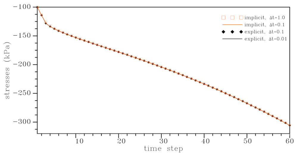
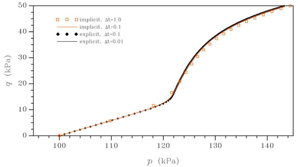
The computing performances of the proposed backward Euler integration were assessed by comparison against the fully explicit formulation proposed in [13] and the fully implicit one recently proposed in [15]. While implicit schemes are unconditionally stable, but generally require an iterative scheme for the solution of the implicit problem generated at each Gauss point, explicit integration schemes are only conditionally stable and require a high number of very small time increments. This drawback could be mitigated by adopting an adaptive sub-stepping technique. The obtained results show the superiority of the proposed backward Euler implementation with respect to the fully explicit references, confirming that the tangent stiffness matrix consistent with the global time integration, as the one derived in this paper, allows for a substantial computational gain in terms of overall analysis time with respect to both the explicit and implicit time integration approaches. It is also worthwhile to emphasize that the original version of the V-N model has a deficiency in the definition of the critical state (see e.g., [9]), but this problem is not addressed in the present paper. Finally, we mention that, while an anisotropic formulation for the V-N model has been provided [27], this work refers to the simpler, isotropic version [10,11].

2. Constitutive Model in Rate Form

Under the assumption of infinitesimal strains, the elasto-viscoplastic constitutive model of [11] is based on the following definition of the effective stress rate, positive if compressive (note that, to simplify the notation and in contrast to what is usually done in soil mechanics, the symbol σ is used to denote the effective stress and not the total stress):

$$\dot{\mathit{\sigma }}\left(t\right)=\mathbf{D}\left(t\right):\left[\dot{\mathit{ϵ}}\left(t\right)-{\dot{\mathit{ϵ}}}^{vp}\left(t\right)\right]$$

(1)

where t is the physical time, σ denotes the effective stress, e the total strain, and D the isotropic elastic tensor:

$$\mathbf{D}\left(t\right)=2G\left(t\right)\mathbf{I}\mathbf{I}+\left[K\left(t\right)-\frac{2}{3}G\left(t\right)\right]\mathbf{I}\otimes \mathbf{I}$$

(2)

where I is the second-order identity tensor and II is the fourth-order tensor of Cartesian components:

$${\left[II\right]}_{ijhk}={\delta }_{ih}{\delta }_{jk}+{\delta }_{ik}{\delta }_{jh}i,j,h,k=1,2,3$$

(3)

G and K are the shear and bulk modulus, respectively. Finally, ${\dot{\mathit{ϵ}}}^{vp}$ in (1) is the viscoplastic strain rate:

$${\dot{\mathit{ϵ}}}^{vp}=\dot{\gamma }\frac{\partial p^{\mathrm{eq}}}{\partial \mathit{\sigma }}$$

(4)

$\dot{\gamma }$ is a scalar viscoplastic multiplier, introduced for convenience of notation, and $p^{\mathrm{eq}}$ is the plastic potential, defined as:

$$\begin{array}{c}\hfill \dot{\gamma }=\frac{{\mu }^{*}}{\tau }\frac{1}{p_{,p}^{eq}}{\left({\displaystyle \frac{p^{\mathrm{eq}}}{p_p^{\mathrm{eq}}}}\right)}^{\frac{{\lambda }^{*}-{\kappa }^{*}}{{\mu }^{*}}}\\ \hfill p^{\mathrm{eq}}(p,q)=p+\frac{q^2}{M^{2}p}\end{array}$$

(5)

In (5), a comma denotes the partial derivative with respect to the variable after the comma, $\tau$ and the non-dimensional parameters ${\mu }^{*}$, ${\lambda }^{*}$, and ${\kappa }^{*}$ are material parameters, which will be defined below, $p=\mathit{\sigma }:\mathbf{I}/3$ is the effective hydrostatic pressure, $q=\sqrt{3/2\mathbf{s}:\mathbf{s}}$ is the effective deviatoric stress, s being the deviatoric stress tensor, and M is the slope of the critical state line in the $q-p$ plane (see Figure 1). Finally, $p_p^{eq}$ (note that in this case, there is no comma before the subscript p) is an internal variable, to be interpreted as a generalized consolidation pressure, governing the hardening behavior of the viscoplastic response.

$\tau$, ${\mu }^{*}$, ${\lambda }^{*}$, and ${\kappa }^{*}$ are material parameters with a clear physical meaning and easily identifiable through standard laboratory tests, such as odometric tests. $\tau$ is a characteristic time, usually set equal to 24 h. ${\mu }^{*}$ is the modified creep index (modified because it is expressed in terms of the volumetric strain rather than the void ratio), which can be obtained in the long term from: (i) the slope of volumetric strain ${ϵ}_v$ versus the logarithm of time [11] (see Figure 2a), (ii) the slope of the inverse of volumetric strain rate versus time (see [28]), and (iii) the slope of logarithm of strain rate versus strain (see [29]), while ${\lambda }^{*}$ is the modified compression index, measuring the slope of the normal consolidation line in the ${ϵ}_v-logp$ plane (see Figure 2b), and ${\kappa }^{*}$ is the modified swelling index, measuring the slope of the unloading or swelling curve in the same plot. The parameters ${\lambda }^{*}$ and ${\kappa }^{*}$ should not be confused with the more commonly used $\lambda$ and $\kappa$ (without the ${}^{*}$ at the apex): Equation (31) in [11] states their relationships (it is ${\lambda }^{*}=\lambda /(1+e)$ and ${\kappa }^{*}=\kappa /(1+e)$, where e is the void ratio).

The evolution of the consolidation pressure, $p_p^{eq}$ in (5), is governed by the following law:

$$p_p^{\mathrm{eq}}=p_{p0}^{\mathrm{eq}}exp\left(\frac{{ϵ}_v^{vp}}{{\lambda }^{*}-{\kappa }^{*}}\right)$$

(6)

where ${ϵ}_v^{vp}$ is the volumetric viscoplastic strain and $p_{p0}^{\mathrm{eq}}$ is a reference parameter defining the initial value of the consolidation pressure. Figure 1 shows two contour plots of $p^{eq}$ in the $q-p$ plane, the original one and an evolved state. The critical state line of slope M is also shown in the plot. Equation (6) shows that the evolution of the plastic potential is independent of the deviatoric component of stress and, together with (4), defines an associative evolution of the viscoplastic strains. It should be noted that these inelastic strains start to develop whenever $p^{\mathrm{eq}}>0$, though, due to the power law in (5), for common values of the parameters, the growth rate is very small as long as $p^{\mathrm{eq}}/p_p^{\mathrm{eq}}<1$.

In general, both G and K in (2) are taken to depend on the current pressure state $p\left(t\right)$, and hence on time, through the following relation:

$$K\left(t\right)=\frac{p\left(t\right)}{{\kappa }^{*}},G\left(t\right)=\frac{3}{2}\frac{1-2\nu }{1+\nu }\frac{p\left(t\right)}{{\kappa }^{*}}$$

(7)

$\nu$ being Poisson’s coefficient.

For the subsequent developments, it is convenient to introduce the projector operators m and n defined as:

$$\mathbf{m}=\frac{\partial p}{\partial }=\frac{1}{3}\mathbf{I},\mathbf{n}=\frac{\partial q}{\partial }=\frac{\partial q}{\partial \mathbf{s}}=\frac{3}{2}\frac{\mathbf{s}}{q}$$

(8)

such that:

$$p=\mathbf{m}:\mathit{\sigma },q=\mathbf{n}:\mathit{\sigma },\mathbf{m}:\mathbf{D}=3K\mathbf{m},\mathbf{n}:\mathbf{D}=2G\mathbf{n}$$

(9)

Following [20], the key idea is that, by using m and n, the viscoplastic strain rate can be easily decomposed into its volumetric and deviatoric components:

$${\dot{\mathit{ϵ}}}^{vp}=\dot{\gamma }\frac{\partial p^{\mathrm{eq}}}{\partial \mathit{\sigma }}=\dot{\gamma }\left(p_{,p}^{\mathrm{eq}}\mathbf{m}+p_{,q}^{\mathrm{eq}}\mathbf{n}\right)$$

(10)

Noting that $\mathbf{m}:\mathbf{n}=0$, $\mathbf{m}:\mathbf{m}=1/3$, and $\mathbf{n}:\mathbf{n}=3/2$, the rates of the stress invariants p and q can be directly obtained from (1), (4), and (10) as:

$$\begin{array}{cc}\hfill \dot{p}& =\mathbf{m}:\mathbf{D}:\dot{\mathit{ϵ}}-\mathbf{m}:\mathbf{D}:\left(p_{,p}^{\mathrm{eq}}\mathbf{m}+p_{,q}^{\mathrm{eq}}\mathbf{n}\right)\dot{\gamma }={\dot{p}}^{\mathrm{trial}}-K{p}_{,p}^{\mathrm{eq}}\dot{\gamma }\hfill \end{array}$$

(11)

$$\begin{array}{cc}\hfill \dot{q}& =\mathbf{n}:\mathbf{D}:\dot{\mathit{ϵ}}-\mathbf{n}:\mathbf{D}:\left(p_{,p}^{\mathrm{eq}}\mathbf{m}+p_{,q}^{\mathrm{eq}}\mathbf{n}\right)\dot{\gamma }={\dot{q}}^{\mathrm{trial}}-3G{p}_{,q}^{\mathrm{eq}}\dot{\gamma }\hfill \end{array}$$

(12)

In (12), ${\dot{p}}^{\mathrm{trial}}=K{\dot{ϵ}}_v/3$ and ${\dot{q}}^{\mathrm{trial}}=2G\mathbf{n}:\dot{\mathit{ϵ}}$ (and hence, also ${\dot{\mathit{\sigma }}}^{\mathrm{trial}}=\mathbf{D}:\dot{\mathit{ϵ}}$) represent tentative values of the stress rates under the assumption of a purely elastic stress variation. In view of the already mentioned absence of a stress threshold for the activation of the viscoplastic strains, a purely elastic stress variation is impossible and, therefore, the trial quantities are purely theoretical.

Equation (10) implicitly defines the rate of the volumetric viscoplastic strain as:

$${\dot{ϵ}}_v^{vp}=p_{,p}^{\mathrm{eq}}\dot{\gamma }$$

(13)

whose integration is required to compute the evolution of the internal variable $p_p^{\mathrm{eq}}$ in (6).

3. Implicit Backward-Difference Time Integration

Let $\Delta t=t^{n+1}-t^n>0$, with $t^n$, $t^{n+1}\in [0-T]$, a time interval along which the constitutive law (1) has to be integrated. A fully implicit, backward-difference scheme is adopted here, whereby all the quantities are evaluated at the end $t^{n+1}$ of the step, whereas the state of the system is assumed to be completely known at $t^n$. In the following derivations, the isotropic elastic tensor D is considered constant in the time step, as is commonly assumed in the literature; see, e.g., [20]. Its value will be updated based on Equation (7) only at the end of the considered time step. An implicit formulation of the algorithm considering also the evolution of D within the time step would be possible, at the cost however of additional complications in the formulation of the integration scheme and of the consequent increase of the computing time, with little expected improvement of accuracy.

The stress at the end of the step can be expressed as:

$${\mathit{\sigma }}^{n+1}={\mathit{\sigma }}^{\mathrm{trial}}-\mathbf{D}:\Delta {\mathit{ϵ}}^{vp}$$

(14)

where ${\mathit{\sigma }}^{\mathrm{trial}}=\mathbf{D}:\left({\mathit{ϵ}}^{n+1}-{\mathit{ϵ}}^{vpn}\right)$ is the stress value at the end of the step under the theoretical assumption of a purely elastic increment and ${\mathit{ϵ}}^{n+1}$ is assumed to be a prescribed quantity. The symbol $\Delta$ will be used to denote the finite increments of all quantities between $t^n$ and $t^{n+1}$.

From (10), the increment of viscoplastic strains is expressed as:

$$\Delta {\mathit{ϵ}}^{vp}=\Delta \gamma {\left(\frac{\partial p^{\mathrm{e}q}}{\partial \mathit{\sigma }}\right)}^{n+1}=\Delta \gamma \left[{\left(p_{,p}^{\mathrm{eq}}\right)}^{n+1}\mathbf{m}+{\left(p_{,q}^{\mathrm{eq}}\right)}^{n+1}{\mathbf{n}}^{n+1}\right]$$

(15)

Exploiting the well-known property for which ${\mathbf{n}}^{n+1}={\mathbf{n}}^{\mathrm{trial}}=(3/2){\mathbf{s}}^{\mathrm{trial}}/q^{\mathrm{trial}}$ (see Appendix A), with $q^{\mathrm{trial}}=\sqrt{3/2{\mathbf{s}}^{\mathrm{trial}}:{\mathbf{s}}^{\mathrm{trial}}}$, the increment of viscoplastic strains can be written as:

$$\Delta {\mathit{ϵ}}^{vp}=\Delta {ϵ}_v^{vp}\mathbf{m}+\Delta e^{vp}\mathbf{n}$$

(16)

with:

$$\Delta {ϵ}_v^{vp}=\Delta \gamma {\left(p_{,p}^{eq}\right)}^{n+1},\Delta e^{vp}=\Delta \gamma {\left(p_{,q}^{eq}\right)}^{n+1}$$

(17)

and the notation $\mathit{n}$ is used instead of ${\mathit{n}}^{\mathrm{trial}}$. Based on (12), the hydrostatic and deviatoric invariants are in turn written as:

$$p^{n+1}=p^{\mathrm{trial}}-K\Delta {ϵ}_v^{vp},q^{n+1}=q^{\mathrm{trial}}-3G\Delta e^{vp}$$

(18)

According to the definition (5) of $\dot{\gamma }$, the increments of the volumetric viscoplastic strain (13) and of the internal variable ${\left(p_p^{\mathrm{eq}}\right)}^{n+1}$ (6) at the end of the step are given by:

$$\begin{array}{cc}\hfill \Delta {ϵ}_v^{vp}& ={\left(p_{,p}^{\mathrm{eq}}\right)}^{n+1}\Delta \gamma =\frac{{\mu }^{*}}{\tau }\Delta t{\left[{\left(\frac{p^{\mathrm{eq}}}{p_p^{\mathrm{eq}}}\right)}^{n+1}\right]}^{\frac{{\lambda }^{*}-{\kappa }^{*}}{{\mu }^{*}}}\hfill \\ \hfill {\left(p_p^{\mathrm{eq}}\right)}^{n+1}& =p_{p0}^{\mathrm{eq}}exp\left(\frac{{ϵ}_v^{vpn}+\Delta {ϵ}_v^{vp}}{{\lambda }^{*}-{\kappa }^{*}}\right)\hfill \end{array}$$

(19)

Using (13), one can express the increment of the plastic multiplier as:

$$\Delta \gamma =\frac{\Delta {ϵ}_v^{vp}}{{\left(p_{,p}^{eq}\right)}^{n+1}}=\frac{{\mu }^{*}}{\tau }\frac{\Delta t}{{\left(p_{,p}^{eq}\right)}^{n+1}}{\left[{\left(\frac{p^{\mathrm{eq}}}{p_p^{\mathrm{eq}}}\right)}^{n+1}\right]}^{\frac{{\lambda }^{*}-{\kappa }^{*}}{{\mu }^{*}}}$$

(20)

and use this expression for the computation of $\Delta e^{vp}$ in (17).

The local non-linear problem defined by Equations (16)–(20) is solved at each Gauss point in an iterative way using the Newton–Raphson method. Once the values $p^{n+1}$, $q^{n+1}$ in (18) have been computed, the value of the stress at the end of the step is determined as:

$${\mathit{\sigma }}^{n+1}={\mathbf{s}}^{n+1}+p^{n+1}\mathbf{I}=\frac{2}{3}{q}^{n+1}\mathbf{n}+p^{n+1}\mathbf{I}$$

(21)

The selected unknowns are collected in the vector ${\displaystyle \mathit{X}}$ defined as:

$$\begin{array}{c}{\displaystyle \mathbf{X}}\\ (5\times 1)\end{array}={\left[\begin{array}{ccccc}\Delta e^{vp}& \Delta {ϵ}_v^{vp}& {\left(p_p^{\mathrm{eq}}\right)}^{n+1}& p^{n+1}& q^{n+1}\end{array}\right]}^T$$

(22)

whose corresponding residuals are:

$$\begin{array}{cc}\hfill {\mathrm{\Psi }}_1& =\Delta e^{vp}-{\left(p_{,q}^{\mathrm{eq}}\right)}^{n+1}\frac{\Delta {ϵ}_v^{vp}}{{\left(p_{,p}^{eq}\right)}^{n+1}}=0\hfill \end{array}$$

(23)

$$\begin{array}{cc}\hfill {\mathrm{\Psi }}_2& =\Delta {ϵ}_v^{vp}-\frac{{\mu }^{*}}{\tau }\Delta t{\left[{\left(\frac{p^{\mathrm{eq}}}{p_p^{\mathrm{eq}}}\right)}^{n+1}\right]}^{\frac{{\lambda }^{*}-{\kappa }^{*}}{{\mu }^{*}}}=0\hfill \end{array}$$

(24)

$$\begin{array}{cc}\hfill {\mathrm{\Psi }}_3& ={\left(p_p^{\mathrm{eq}}\right)}^{n+1}-p_{p0}^{\mathrm{eq}}exp\left(\frac{{ϵ}_v^{vpn}+\Delta {ϵ}_v^P}{{\lambda }^{*}-{\kappa }^{*}}\right)=0\hfill \end{array}$$

(25)

$$\begin{array}{cc}\hfill {\mathrm{\Psi }}_4& =p^{n+1}-p^{\mathrm{trial}}+K\Delta {ϵ}_v^{vp}=0\hfill \end{array}$$

(26)

$$\begin{array}{cc}\hfill {\mathrm{\Psi }}_5& =q^{n+1}-q^{\mathrm{trial}}+3G\Delta e^{vp}=0\hfill \end{array}$$

(27)

For convenience, these can be collected in a residual vector ${\displaystyle \mathrm{\Psi }}$:

$$\begin{array}{c}{\displaystyle \mathrm{\Psi }}\\ (5\times 1)\end{array}={\left[\begin{array}{ccccc}{\mathrm{\Psi }}_1& {\mathrm{\Psi }}_2& {\mathrm{\Psi }}_3& {\mathrm{\Psi }}_4& {\mathrm{\Psi }}_5\end{array}\right]}^T$$

(28)

The trial values in (26) and in (27) are given by:

$$\begin{array}{cc}\hfill {\mathit{\sigma }}^{\mathrm{trial}}& =\mathbf{D}:\left({\mathit{ϵ}}^{n+1}-{\mathit{ϵ}}^{vpn}\right),p^{\mathrm{trial}}=\mathbf{m}:{\mathit{\sigma }}^{\mathrm{trial}},{\mathbf{s}}^{\mathrm{trial}}=\mathbf{n}:{\mathit{\sigma }}^{\mathrm{trial}},\hfill \\ \hfill q^{\mathrm{trial}}& =\sqrt{\frac{3}{2}{\mathit{s}}^{\mathrm{trial}}:{\mathit{s}}^{\mathrm{trial}}}\hfill \end{array}$$

(29)

It should be noted that not all residuals explicitly depend on all unknowns, as can be seen below:

$$\begin{array}{cc}\hfill {\mathrm{\Psi }}_1& ={\mathrm{\Psi }}_1\left(\Delta e^{vp},\Delta {ϵ}_v^{vp},p^{n+1},q^{n+1}\right)\hfill \end{array}$$

(30)

$$\begin{array}{cc}\hfill {\mathrm{\Psi }}_2& ={\mathrm{\Psi }}_2\left(\Delta {ϵ}_v^{vp},{\left(p_p^{\mathrm{eq}}\right)}^{n+1},p^{n+1},q^{n+1}\right)\hfill \end{array}$$

(31)

$$\begin{array}{cc}\hfill {\mathrm{\Psi }}_3& ={\mathrm{\Psi }}_3\left(\Delta {ϵ}_v^{vp},{\left(p_p^{\mathrm{eq}}\right)}^{n+1}\right)\hfill \end{array}$$

(32)

$$\begin{array}{cc}\hfill {\mathrm{\Psi }}_4& ={\mathrm{\Psi }}_4\left(\Delta {ϵ}_v^{vp},p^{n+1}\right)\hfill \end{array}$$

(33)

$$\begin{array}{cc}\hfill {\mathrm{\Psi }}_5& ={\mathrm{\Psi }}_5\left(\Delta e^{vp},q^{n+1}\right)\hfill \end{array}$$

(34)

Proceeding iteratively with a first-order linearization of the resolving system, at the $(i+1)$-th iteration, one has:

$${\displaystyle {{\Psi }}_{i+1}\cong {{\Psi }}_i+{\left.\frac{d{\Psi }}{d\mathit{X}}\right|}_i\delta \mathit{X}=\mathbf{0}}$$

(35)

where ${{\Psi }}_i$ defines the residual vector at iteration i and ${\displaystyle \delta \mathit{X}}$ is the increment of the unknown variables between two subsequent iterations:

$$\begin{array}{c}{\displaystyle \delta \mathit{X}}\\ (5\times 1)\end{array}={\left[\begin{array}{ccccc}\delta \Delta e^{vp}& \delta \Delta {ϵ}_v^{vp}& \delta p_p^{\mathrm{eq}}& \delta p& \delta q\end{array}\right]}^T$$

(36)

The residual gradient $d{\Psi }/d\mathit{X}$ is a $5\times 5$ matrix containing the derivatives of the residuals w.r.t. the unknowns. Its detailed expression is given in Appendix B. It can be shown that the gradient $d{\Psi }/d\mathit{X}$ is non-symmetric. Consequently, a non-symmetric solver must be used for the local problem, if a consistent tangent matrix is desired to assure an asymptotic quadratic convergence.

4. Consistent Tangent Stiffness

Starting from the known material state at $t^{n+1}$, a virtual total stress variation $\delta \mathit{\sigma }$ occurring in the infinitesimal time $\delta t$ can be expressed as (since all quantities are evaluated at $t^{n+1}$, the superscript $n+1$ is omitted to simplify the notation):

$$\begin{array}{c}\hfill \delta \mathit{\sigma }=\frac{\partial \mathit{\sigma }}{\partial \mathit{ϵ}}:\delta \mathit{ϵ}+\frac{\partial \mathit{\sigma }}{\partial t}\delta t\end{array}$$

(37)

where the term $\partial \mathit{\sigma }/\partial t·\delta t$ accounts for the viscous stress relaxation at constant strains. Using (21), the stress variation $\delta \mathit{\sigma }$ can also be written as:

$$\delta \mathit{\sigma }=\frac{2}{3}\mathbf{n}\delta q+\frac{2}{3}q\delta \mathbf{n}+\mathbf{I}\delta p=\frac{2}{3}\mathbf{n}\left(\frac{\partial q}{\partial \mathit{ϵ}}:\delta \mathit{ϵ}+\frac{\partial q}{\partial t}\delta t\right)+\frac{2}{3}q\frac{\partial \mathbf{n}}{\partial \mathit{ϵ}}:\delta \mathit{ϵ}+\left(\mathbf{I}\frac{\partial p}{\partial \mathit{ϵ}}:\delta \mathit{ϵ}+\mathbf{I}\frac{\partial p}{\partial t}\delta t\right)$$

(38)

After reordering, we obtain:

$$\delta \mathit{\sigma }=\underset{{\displaystyle \frac{\partial \mathit{\sigma }}{\partial \mathit{ϵ}}}}{\underbrace{\left(\frac{2}{3}\mathbf{n}\otimes \frac{\partial q}{\partial \mathit{ϵ}}+\frac{2}{3}q\frac{\partial \mathbf{n}}{\partial \mathit{ϵ}}+\mathbf{I}\otimes \frac{\partial p}{\partial \mathit{ϵ}}\right)}}:\delta \mathit{ϵ}+\underset{{\displaystyle \frac{\partial \mathit{\sigma }}{\partial t}}}{\underbrace{\left(\frac{2}{3}\mathbf{n}\frac{\partial q}{\partial t}+\mathbf{I}\frac{\partial p}{\partial t}\right)}}\delta t$$

(39)

The first term $\partial \mathit{\sigma }/\partial ϵ$ is the contribution to the global tangent matrix to be used in the finite element code (i.e., in an UMAT user subroutine in the software Abaqus™).

The computation of (39) requires the derivation of $\delta \mathbf{n}$, $\delta p$, and $\delta q$ in terms of $\delta \mathit{ϵ}$ and $\delta t$ n does not depend on time and its variation with $\delta$ can be obtained starting from its definition (8)${}_2$:

$$\delta \mathbf{n}=\frac{3}{2}\left(\frac{1}{q^{\mathrm{trial}}}\delta {\mathbf{s}}^{\mathrm{trial}}-\frac{{\mathbf{s}}^{\mathrm{trial}}}{{q^{\mathrm{trial}}}^2}\delta q^{\mathrm{trial}}\right)$$

(40)

with:

$$\begin{array}{cc}\hfill \delta {\mathbf{s}}^{\mathrm{trial}}& =2G\mathbf{Dev}:\delta \mathit{ϵ}\hfill \\ \hfill \delta q^{\mathrm{trial}}& =\frac{\partial q^{\mathrm{trial}}}{{\partial \mathbf{s}}^{\mathrm{trial}}}:\delta {\mathbf{s}}^{\mathrm{trial}}=2G\mathbf{n}:\mathbf{Dev}:\delta \mathit{ϵ}=2G\mathbf{n}:\delta \mathit{ϵ}\hfill \end{array}$$

(41)

where $\mathbf{Dev}$ is the deviatoric operator defined as:

$$\mathbf{Dev}=\mathbf{I}\mathbf{I}-\frac{1}{3}\mathbf{I}\otimes \mathbf{I}$$

(42)

Replacing (41) in (40) and taking into account that ${\mathbf{s}}^{\mathrm{trial}}=2/3q^{\mathrm{trial}}\mathbf{n}$, one has:

$$\delta \mathbf{n}=\frac{3G}{q^{\mathrm{trial}}}\left(\mathbf{Dev}-\frac{2}{3}\mathbf{n}\otimes \mathbf{n}\right):\delta \mathit{ϵ}$$

(43)

The variations $\delta p$ and $\delta q$ are obtained from (18) and (17):

$$\begin{array}{cc}\hfill \delta p& =\delta p^{\mathrm{trial}}-K\left(p_{,pp}^{\mathrm{eq}}\delta p+p_{,pq}^{\mathrm{eq}}\delta q\right)\Delta \gamma -K{p}_{,p}^{\mathrm{eq}}\delta \Delta \gamma \hfill \\ \hfill \delta q& =\delta q^{\mathrm{trial}}-3G\left(p_{,qp}^{\mathrm{eq}}\delta p+p_{,qq}^{\mathrm{eq}}\delta q\right)\Delta \gamma -3G{p}_{,q}^{\mathrm{eq}}\delta \Delta \gamma \hfill \end{array}$$

(44)

with $\delta q^{\mathrm{trial}}$ given in (41)${}_2$ and:

$$\delta p^{\mathrm{trial}}=3K\mathbf{m}:\delta \mathit{ϵ}$$

(45)

After rearranging, Equation (44) can be rewritten as:

$$\begin{array}{cc}\hfill \left(1+K{p}_{,pp}^{\mathrm{eq}}\Delta \gamma \right)\delta p+\left(K{p}_{,pq}^{\mathrm{eq}}\Delta \gamma \right)\delta q& =3K\mathbf{m}:\delta \mathit{ϵ}-K{p}_{,p}^{\mathrm{eq}}\delta \Delta \gamma \hfill \\ \hfill \left(3G{p}_{,qp}^{\mathrm{eq}}\Delta \gamma \right)\delta p+\left(1+3G{p}_{,qq}^{\mathrm{eq}}\Delta \gamma \right)\delta q& =2G\mathbf{n}:\delta \mathit{ϵ}-3G{p}_{,q}^{\mathrm{eq}}\delta \Delta \gamma \hfill \end{array}$$

(46)

The computation of $\delta p$ and $\delta q$ in (44) requires the definition of $\delta \Delta \gamma$. This can be obtained from the expression (19)${}_1$ of $\Delta {ϵ}_v^{vp}$:

$$\delta \Delta {ϵ}_v^{vp}=\delta \left(p_{,p}^{\mathrm{eq}}\Delta \gamma \right)=\frac{{\mu }^{*}}{\tau }\Delta t\delta \left[{\left(\frac{p^{\mathrm{eq}}}{p_p^{\mathrm{eq}}}\right)}^{\frac{{\lambda }^{*}-{\kappa }^{*}}{{\mu }^{*}}}\right]+\frac{{\mu }^{*}}{\tau }{\left(\frac{p^{\mathrm{eq}}}{p_p^{\mathrm{eq}}}\right)}^{\frac{{\lambda }^{*}-{\kappa }^{*}}{{\mu }^{*}}}\delta t$$

(47)

with:

$$\begin{array}{cc}\hfill \delta \left(p_{,p}^{\mathrm{eq}}\Delta \gamma \right)& =p_{,pp}^{\mathrm{eq}}\Delta \gamma \delta p+p_{,pq}^{\mathrm{eq}}\Delta \gamma \delta q+p_{,p}^{\mathrm{eq}}\delta \Delta \gamma \hfill \\ \hfill \delta \left[{\left(\frac{p^{\mathrm{eq}}}{p_p^{\mathrm{eq}}}\right)}^{\frac{{\lambda }^{*}-{\kappa }^{*}}{{\mu }^{*}}}\right]& =\frac{{\lambda }^{*}-{\kappa }^{*}}{{\mu }^{*}}{\left(\frac{p^{\mathrm{eq}}}{p_p^{\mathrm{eq}}}\right)}^{\frac{{\lambda }^{*}-{\kappa }^{*}-{\mu }^{*}}{{\mu }^{*}}}\delta \left(\frac{p^{\mathrm{eq}}}{p_p^{\mathrm{eq}}}\right)\hfill \\ \hfill \delta \left(\frac{p^{\mathrm{eq}}}{p_p^{\mathrm{eq}}}\right)& =\frac{1}{p_p^{\mathrm{eq}}}\left(p_{,p}^{\mathrm{eq}}\delta p+p_{,q}^{\mathrm{eq}}\delta q\right)-\frac{p^{\mathrm{eq}}}{{\left(p_p^{\mathrm{eq}}\right)}^2}\delta p_p^{\mathrm{eq}}\hfill \\ \hfill \delta p_p^{\mathrm{eq}}& =\frac{1}{{\lambda }^{*}-{\mu }^{*}}{\left(p_p^{\mathrm{eq}}\right)}^{n}exp\left(\frac{\Delta {ϵ}_v^{vp}}{{\lambda }^{*}-{\mu }^{*}}\right)\delta \Delta {ϵ}_v^{vp}\hfill \end{array}$$

(48)

Replacing (48)${}_{2,3,4}$ in (47), one has:

$$\begin{array}{cc}\hfill \delta \Delta {ϵ}_v^{vp}& =\frac{\Delta t}{\tau }\left({\lambda }^{*}-{\kappa }^{*}\right){\left[\frac{p^{\mathrm{eq}}}{p_p^{\mathrm{eq}}}\right]}^{\frac{{\lambda }^{*}-{\kappa }^{*}-{\mu }^{*}}{{\mu }^{*}}}·\hfill \\ \hfill & ·\left[\frac{\left(p_{,p}^{\mathrm{eq}}\delta p+p_{,q}^{\mathrm{eq}}\delta q\right)}{p_p^{\mathrm{eq}}}-\frac{p^{\mathrm{eq}}}{{\left(p_p^{\mathrm{eq}}\right)}^2}\frac{{\left(p_p^{\mathrm{eq}}\right)}^n}{{\lambda }^{*}-{\mu }^{*}}exp\left(\frac{\Delta {ϵ}_v^{vp}}{{\lambda }^{*}-{\mu }^{*}}\right)\delta \Delta {ϵ}_v^{vp}\right]+\hfill \\ \hfill & +\frac{{\mu }^{*}}{\tau }{\left[\frac{p^{\mathrm{eq}}}{p_p^{\mathrm{eq}}}\right]}^{\frac{{\lambda }^{*}-{\kappa }^{*}}{{\mu }^{*}}}\delta t\hfill \end{array}$$

(49)

Rearranging the different terms, Equation (49) can be rewritten as:

$$A\delta \Delta {ϵ}_v^P=B\left(p_{,p}^{\mathrm{eq}}\delta p+p_{,q}^{\mathrm{eq}}\delta q\right)+\frac{{\mu }^{*}}{\tau }{\left(\frac{p^{\mathrm{eq}}}{p_p^{\mathrm{eq}}}\right)}^{\frac{{\lambda }^{*}-{\kappa }^{*}}{{\mu }^{*}}}\delta t$$

(50)

with

$$\begin{array}{cc}\hfill B& =\Delta t\frac{{\lambda }^{*}-{\kappa }^{*}}{\tau }{\left(\frac{p^{\mathrm{eq}}}{p_p^{\mathrm{eq}}}\right)}^{\frac{{\lambda }^{*}-{\kappa }^{*}-{\mu }^{*}}{{\mu }^{*}}}·\frac{1}{p_p^{\mathrm{eq}}}\hfill \end{array}$$

(51)

$$\begin{array}{cc}\hfill A& =1+B\left(\frac{p^{\mathrm{eq}}}{p_p^{\mathrm{eq}}}\right)\frac{{\left(p_p^{\mathrm{eq}}\right)}^n}{{\lambda }^{*}-{\kappa }^{*}}exp\left(\frac{\Delta {ϵ}_v^{vp}}{{\lambda }^{*}-{\mu }^{*}}\right)\hfill \end{array}$$

(52)

From (47), (48)${}_1$, and (50), one can write:

$$A{p}_{,pp}^{\mathrm{eq}}\Delta \gamma \delta p+A{p}_{,pq}^{\mathrm{eq}}\Delta \gamma \delta q+A{p}_{,p}^{\mathrm{eq}}\delta \Delta \gamma =B\left(p_{,p}^{\mathrm{eq}}\delta p+p_{,q}^{\mathrm{eq}}\delta q\right)+\frac{{\mu }^{*}}{\tau }{\left[\frac{p^{\mathrm{eq}}}{p_p^{\mathrm{eq}}}\right]}^{\frac{{\lambda }^{*}-{\kappa }^{*}}{{\mu }^{*}}}\delta t$$

(53)

and then solve for $\delta \Delta \gamma$:

$$\delta \Delta \gamma =\frac{1}{A{p}_{,p}^{\mathrm{eq}}}\left[B{p}_{,p}^{\mathrm{eq}}-A{p}_{,pp}^{\mathrm{eq}}\Delta \gamma \right]\delta p+\frac{1}{A{p}_{,p}^{\mathrm{eq}}}\left[B{p}_{,q}^{\mathrm{eq}}-A{p}_{,pq}^{\mathrm{eq}}\Delta \gamma \right]\delta q+\frac{1}{A{p}_{,p}^{\mathrm{eq}}}\frac{{\mu }^{*}}{\tau }{\left[\frac{p^{\mathrm{eq}}}{p_p^{\mathrm{eq}}}\right]}^{\frac{{\lambda }^{*}-{\kappa }^{*}}{{\mu }^{*}}}\delta t$$

(54)

The present expression of $\delta \Delta \gamma$ can be replaced in (46), obtaining (after some algebra) the following system of equations in the unknown variations $\delta p$ and $\delta q$:

$$\begin{array}{cc}\hfill F_{11}\delta p+F_{12}\delta q& =3K\mathbf{m}:\delta \mathit{ϵ}-\frac{K}{A}\frac{{\mu }^{*}}{\tau }{\left[\frac{p^{\mathrm{eq}}}{p_p^{\mathrm{eq}}}\right]}^{\frac{{\lambda }^{*}-{\kappa }^{*}}{{\mu }^{*}}}\delta t\hfill \\ \hfill F_{21}\delta p+F_{22}\delta q& =2G\mathbf{n}:\delta \mathit{ϵ}-3G\frac{p_{,q}^{\mathrm{eq}}}{A{p}_{,p}^{\mathrm{eq}}}\frac{{\mu }^{*}}{\tau }{\left[\frac{p^{\mathrm{eq}}}{p_p^{\mathrm{eq}}}\right]}^{\frac{{\lambda }^{*}-{\kappa }^{*}}{{\mu }^{*}}}\delta t\hfill \end{array}$$

(55)

with:

$$\begin{array}{cc}\hfill F_{11}& =1+K{p}_{,pp}^{\mathrm{eq}}\frac{B}{A}\hfill \\ \hfill F_{12}& =K{p}_{,q}^{\mathrm{eq}}\frac{B}{A}\hfill \\ \hfill F_{21}& =3G{p}_{,qp}^{\mathrm{eq}}\Delta \gamma +3G{p}_{,q}^{\mathrm{eq}}\frac{B}{A}-3G{p}_{,q}^{\mathrm{eq}}\frac{p_{,q}^{\mathrm{eq}}}{p_{,p}^{\mathrm{eq}}}{p}_{,pp}^{\mathrm{eq}}\Delta \gamma \hfill \\ \hfill F_{22}& =1+3G{p}_{,qq}^{\mathrm{eq}}\Delta \gamma +3G\frac{{\left(p_{,q}^{\mathrm{eq}}\right)}^2}{p_{,p}^{\mathrm{eq}}}\frac{B}{A}-3G\frac{p_{,q}^{\mathrm{eq}}}{p_{,p}^{\mathrm{eq}}}{p}_{,pq}^{\mathrm{eq}}\frac{B}{A}\Delta \gamma \hfill \end{array}$$

(56)

The system (55) can be solved analytically for $\delta p$ and $\delta q$:

$$\begin{array}{cc}\hfill \delta p& =c_{11}\left(3K\mathbf{m}:\delta ϵ-\frac{K}{A}\frac{{\mu }^{*}}{\tau }{\left[\frac{p^{\mathrm{eq}}}{p_p^{\mathrm{eq}}}\right]}^{\frac{{\lambda }^{*}-{\kappa }^{*}}{{\mu }^{*}}}\delta t\right)+c_{12}\left(2G\mathbf{n}:\delta ϵ-3G\frac{p_{,q}^{\mathrm{eq}}}{A{p}_{,p}^{\mathrm{eq}}}\frac{{\mu }^{*}}{\tau }{\left[\frac{p^{\mathrm{eq}}}{p_p^{\mathrm{eq}}}\right]}^{\frac{{\lambda }^{*}-{\kappa }^{*}}{{\mu }^{*}}}\delta t\right)\hfill \\ \hfill \delta q& =c_{21}\left(3K\mathbf{m}:\delta ϵ-\frac{K}{A}\frac{{\mu }^{*}}{\tau }{\left[\frac{p^{\mathrm{eq}}}{p_p^{\mathrm{eq}}}\right]}^{\frac{{\lambda }^{*}-{\kappa }^{*}}{{\mu }^{*}}}\delta t\right)+c_{22}\left(2G\mathbf{n}:\delta ϵ-3G\frac{p_{,q}^{\mathrm{eq}}}{A{p}_{,p}^{\mathrm{eq}}}\frac{{\mu }^{*}}{\tau }{\left[\frac{p^{\mathrm{eq}}}{p_p^{\mathrm{eq}}}\right]}^{\frac{{\lambda }^{*}-{\kappa }^{*}}{{\mu }^{*}}}\delta t\right)\hfill \end{array}$$

(57)

where the terms $c_{11}$, $c_{12}$, $c_{21}$, $c_{22}$ are the coefficients of the matrix $\mathit{C}={\mathit{F}}^{-1}$, namely:

$$\mathbf{C}=\left[\begin{array}{cc}{c}_{11}& c_{12}\\ c_{21}& c_{22}\end{array}\right]={\mathit{F}}^{-1}=\frac{1}{det\mathit{F}}\left[\begin{array}{cc}{F}_{22}& -F_{12}\\ -F_{21}& F_{11}\end{array}\right]$$

(58)

Rearranging (57), one obtains:

$$\begin{array}{cc}\hfill \delta p& =\left[c_{11}K\mathbf{I}+c_{12}2G\mathbf{n}\right]:\delta ϵ-\left[c_{11}\frac{K}{A}\frac{{\mu }^{*}}{\tau }{\left(\frac{p^{\mathrm{eq}}}{p_p^{\mathrm{eq}}}\right)}^{\frac{{\lambda }^{*}-{\kappa }^{*}}{{\mu }^{*}}}+c_{12}3G\frac{p_{,q}^{\mathrm{eq}}}{A{p}_{,p}^{\mathrm{eq}}}\frac{{\mu }^{*}}{\tau }{\left(\frac{p^{\mathrm{eq}}}{p_p^{\mathrm{eq}}}\right)}^{\frac{{\lambda }^{*}-{\kappa }^{*}}{{\mu }^{*}}}\right]:\delta t\hfill \\ \hfill \delta q& =\left[c_{21}K\mathbf{I}+c_{22}2G\mathbf{n}\right]:\delta ϵ-\left[c_{21}\frac{K}{A}\frac{{\mu }^{*}}{\tau }{\left(\frac{p^{\mathrm{eq}}}{p_p^{\mathrm{eq}}}\right)}^{\frac{{\lambda }^{*}-{\kappa }^{*}}{{\mu }^{*}}}+c_{22}3G\frac{p_{,q}^{\mathrm{eq}}}{A{p}_{,p}^{\mathrm{eq}}}\frac{{\mu }^{*}}{\tau }{\left(\frac{p^{\mathrm{eq}}}{p_p^{\mathrm{eq}}}\right)}^{\frac{{\lambda }^{*}-{\kappa }^{*}}{{\mu }^{*}}}\right]:\delta t\hfill \end{array}$$

(59)

Replacing the obtained expressions of $\delta \mathbf{n}$ (43), $\delta p$ (59)${}_1$, and $\delta q$ (59)${}_2$ in (37), one finally obtains the explicit expression of the tangent matrix:

$$\begin{array}{cc}\hfill \delta \mathit{\sigma }& =\underset{}{\underset{{\displaystyle \frac{\partial \mathit{\sigma }}{\partial \mathit{ϵ}}}}{\left[\left(\frac{2}{3}{c}_{21}K\mathbf{n}\otimes \mathbf{I}+c_{12}2G\mathbf{I}\otimes \mathbf{n}\right)+\frac{4}{3}G\left(c_{22}-\frac{q}{q^{\mathrm{trial}}}\right)\mathbf{n}\otimes \mathbf{n}+2G\frac{q}{q^{\mathrm{trial}}}\mathbf{Dev}+c_{11}K\mathbf{I}\otimes \mathbf{I}\right]}}:\delta \mathit{ϵ}+\hfill \\ & +\{-\mathbf{I}\left[c_{11}\frac{K}{A}\frac{{\mu }^{*}}{\tau }{\left(\frac{p^{\mathrm{eq}}}{p_p^{\mathrm{eq}}}\right)}^{\frac{{\lambda }^{*}-{\kappa }^{*}}{{\mu }^{*}}}+c_{12}3G\frac{p_{,q}^{\mathrm{eq}}}{A{p}_{,p}^{\mathrm{eq}}}\frac{{\mu }^{*}}{\tau }{\left(\frac{p^{\mathrm{eq}}}{p_p^{\mathrm{eq}}}\right)}^{\frac{{\lambda }^{*}-{\kappa }^{*}}{{\mu }^{*}}}\right]+\hfill \\ & -\frac{2}{3}\mathbf{n}\left[c_{21}\frac{K}{A}\frac{{\mu }^{*}}{\tau }{\left(\frac{p^{\mathrm{eq}}}{p_p^{\mathrm{eq}}}\right)}^{\frac{{\lambda }^{*}-{\kappa }^{*}}{{\mu }^{*}}}+c_{22}3G\frac{p_{,q}^{\mathrm{eq}}}{A{p}_{,p}^{\mathrm{eq}}}\frac{{\mu }^{*}}{\tau }{\left(\frac{p^{\mathrm{eq}}}{p_p^{\mathrm{eq}}}\right)}^{\frac{{\lambda }^{*}-{\kappa }^{*}}{{\mu }^{*}}}\right]\}\delta t\hfill \end{array}$$

(60)

The term inside the curly brackets in (60) is the partial derivative of the stress with respect to time, i.e., $\partial \mathit{\sigma }/\partial t$. The stress variation in (60) consists of two contributions. The first, $\partial \mathit{\sigma }/\partial \mathit{ϵ}$, is the tangent stiffness operator to be used for the predictor step in the global Newton–Raphson iteration scheme. This is the term that is required by Abaqus™ to be computed at each Gauss point in a User Material subroutine and to be passed to the code for global iteration. The second term, $\partial \mathit{\sigma }/\partial t$, accounts for the stress relaxation at constant strain and does not have to be passed to Abaqus™ by the User Material subroutine. However, it has to be properly taken into account for the validation of the tangent stiffness operator, as will be discussed in the next section.

It should be noted that the tangent stiffness operator $\partial \mathit{\sigma }/\partial \mathit{ϵ}$ in (60) is not symmetric. However, it can be shown that the coefficients $c_{12}$ and $c_{21}$ of the non-symmetric part in (60) vanish for vanishing $\Delta \gamma$, a result in agreement with the findings in [20].

The implemented procedure is summarized in Algorithms 1–4.

Algorithm 1: Implicit backward difference time integration.

Initialization Solve Newton–Raphson linear System (35) to obtain ${\mathit{\sigma }}^{n+1}$, Equation (21) Compute tangent matrix ${\left(\frac{\partial \mathit{\sigma }}{\partial \mathit{ϵ}}\right)}^{n+1}$, Equation (60)

Algorithm 2: Initialization.

At time step n, from $t_n$ to $t_{n+1}$, all quantities at time $t_n$ are known. Given ${\Delta \mathit{ϵ}}^n$, compute ${\mathit{ϵ}}^{n+1}={\mathit{ϵ}}^n+\Delta {\mathit{ϵ}}^n$. ${\mathbf{n}}^{\mathrm{trial}}$, ${\mathit{\sigma }}^{\mathrm{trial}}$, ${\mathbf{s}}^{\mathrm{trial}}$, $p^{\mathrm{trial}}$ and $q^{\mathrm{trial}}$ from Equations (8)${}_2$ and (29). Initial (trial) values for derivatives of $p^{\mathrm{eq}}$ are then known from Equation (A10).

Algorithm 3: Solve Newton–Raphson linear System (35) to obtain ${\mathit{\sigma }}^{n+1}$.

At iteration i, if $i=0$, use trial values for $n+1$ quantities.

Compute residuals ${\displaystyle {{\Psi }}_i}$ for the linearized system (35) with Equations (23)–(27).

Compute the coefficient matrix ${\displaystyle {\left.\frac{d{\Psi }}{d\mathit{X}}\right|}_i}$ for the linearized system (35) with Equations (A11)–(A13).

Solve linearized System (35) for the unknowns ${\displaystyle \delta \mathit{X}}$ in Equation (36).

Update ${\displaystyle {\mathit{X}}^{i+1}={\mathit{X}}^i+\delta \mathit{X}}$.

Convergence test: if passed, ${\mathit{X}}^{n+1}={\mathit{X}}^{i+1}$, and exit loop. Else, repeat from 1 with ${\mathit{X}}^{i+1}={\mathit{X}}^i$ and $i+1⟶i$.

Algorithm 4: Compute tangent matrix ${\left(\frac{\partial \mathit{\sigma }}{\partial \mathit{ϵ}}\right)}^{n+1}$, Equation (60).

Update at $t^{n+1}$: ${\left(p^{\mathrm{eq}}\right)}^{n+1}$ with Equation (5)${}_2$; derivatives of ${\left(p^{\mathrm{eq}}\right)}^{n+1}$ with

Equation (A10); $K^{n+1}$, $G^{n+1}$ with Equation (7); $p_p^{\mathrm{eq}}$ with Equation (19).

Compute B and A from Equations (51) and (52), respectively.

Compute $F_{11},F_{12},F_{21},F_{22}$ with Equation (56), $det\mathbf{F}=\left(F_{11}·F_{22}-F_{12}·F_{21}\right)$ and the coefficients $c_{11},c_{12},c_{21},c_{22}$ with Equation (58).

Compute the tangent stiffness matrix with Equation (60), here rewritten for clarity

(all quantities are calculated at $t^{n+1}$, if not indicated otherwise):

$$\begin{array}{cc}\hfill {\left(\frac{\partial \mathit{\sigma }}{\partial \mathit{ϵ}}\right)}^{n+1}& =\left(\frac{2}{3}{c}_{21}K\mathbf{n}\otimes \mathbf{I}+c_{12}2G\mathbf{I}\otimes \mathbf{n}\right)+\frac{4}{3}G\left(c_{22}-\frac{q}{q^{\mathrm{trial}}}\right)\mathbf{n}\otimes \mathbf{n}+\hfill \\ \hfill & +2G\frac{q}{q^{\mathrm{trial}}}\mathbf{Dev}+c_{11}K\mathbf{I}\otimes \mathbf{I}\hfill \end{array}$$

5. Numerical Tests

The robustness, accuracy, and efficiency of the proposed model were investigated with numerical tests. The implicit version of the model described in the previous sections was first implemented in a MATLAB™ code and validated at the material point level by imposing a strain history and calculating the corresponding stress. Then, the material model was implemented in a user material subroutine of a commercial finite element code [30] and was applied to the simulation of subsidence at a reservoir scale, as was described in [26]. Finally, the model was tested on a large-scale geomechanical problem. In the tests, the proposed implicit approach was compared both with the explicit integration procedure proposed in [13] and with the implicit one proposed in [15]. When showing the results, the following convention for the stress components was assumed: $\mathit{\sigma }=\left[{\sigma }_{11}{\sigma }_{22}{\sigma }_{33}{\sigma }_{23}{\sigma }_{13}{\sigma }_{12}\right]$.

5.1. Tests at the Material Point Level

The tests at the material point level were performed by imposing a strain history and evaluating the corresponding stresses. The results of the proposed implicit integration scheme were compared with the outcomes of an explicit integration. The material properties used in these tests are shown in

Table 1. Material parameters for the Vermeer–Neher (V-N) law. OCR, overconsolidation ratio.

${\mathit{\kappa }}^{*}$	${\mathit{\lambda }}^{*}$	${\mathit{\mu }}^{*}$	M	$\mathit{\nu }$	OCR	$\mathit{\tau }$ (days)
0.0084	0.061	0.0011	1.33	0.3	1.39	1

, where OCR denotes the overconsolidation ratio, used in the definition of $p_0^{\mathrm{eq}}=\mathrm{OCR}·p_0$, $p_0$ being the initial hydrostatic stress.

In the following examples, the strain history will be imposed by defining the strain increment vector $\Delta$ as:

$$\begin{array}{c}\hfill \Delta \mathit{ϵ}={\overline{\Delta ϵ}}_V\left[{\mathbf{n}}_1+c_1{\mathbf{n}}_2\right]\end{array}$$

(61)

where ${\overline{\Delta ϵ}}_V$ is the desired volumetric strain (to be imposed), ${\mathbf{n}}_1={\left[111000\right]}^T$ (using Voigt’s notation for the stress tensor), $c_1=\frac{Ktan\beta }{2G}$, and $\beta$ defines the relationship between p and q ($\Delta p=tan\beta \Delta q$) in the first increment. The vector ${\mathbf{n}}_2$ defines which stress directions were activated, and it varies from case to case. All the analyses were initialized with a non-zero hydrostatic stress through the parameter $p_0$.

5.1.1. Test 1: Monotonic Loading

In the first test, an increasing strain was imposed at a single Gauss point. Because of the imposed strain path (61), the obtained stress had both a hydrostatic and a deviatoric component. The imposed deformation increment was chosen to activate the stress component in Direction 11, i.e., aligned with the vector ${\mathbf{n}}_2={\left[100000\right]}^T$. The other parameters were: ${\overline{\Delta ϵ}}_V={10}^{-4}$, $\beta ={30}^o$, and $p_0={10}^5$ Pa.

The evolution in time of the stress component ${\sigma }_{11}$ is depicted in Figure 3. To be precise, the stress is plotted as a function of the time step number, where time steps of constant amplitude were used. The curves show an excellent agreement between implicit and explicit integration using a time step $\Delta t=0.1$, where $\Delta t$ is the non-dimensional time step size $\Delta t=(t^{n+1}-t^n)/\overline{\tau }$ and the time units of $\overline{\tau }$ are years. It can be observed that the implicit scheme was able to provide an accurate solution even when using a time step 10 times ($\Delta t=1.0$) larger than the explicit case. When using the same larger time step ($\Delta t=1.0$), the implementation with explicit integration was not able to provide a solution. To confirm the accuracy of the proposed algorithm, an explicit solution with a very small time step ($\Delta t=0.01$) is plotted. No significant difference can be appreciated between the curves.

The same results are subsequently plotted in a $p-q$ plane in Figure 4. In this plane as well, it is possible to observe a very good agreement between the implicit solution with large time step and the explicit one obtained with a much smaller time step. A slight difference is visible in the implicit solution with the larger time step, due to the less frequent evaluation of the stress along the (nonlinear) loading history.

5.1.2. Test 2: Monotonic Loading

The second test was very similar to the previous one, the only difference being the activated stress component. In this second case, the increasing strain activated the stress in Direction 12, i.e., aligned with the vector ${\mathbf{n}}_2={\left[000100\right]}^T$). Figure 5 shows the time evolution of the stress component for two different time step sizes. For the smaller time step ($\Delta t=0.1$), the implicit and explicit results were very close. However, when the time step size increased ($\Delta t=1.0$), the explicit solution tended to oscillate.

The same results can be also observed in a $p-q$ plane in Figure 6. As expected, this test confirmed that the implicit integration scheme was more robust and allowed for the use of a larger time step size, possibly reducing the global computing time of the analysis.

5.1.3. Test 3: Loading and Unloading

In this test, a loading and unloading evolution of the strain was imposed. First, it increased linearly (${\overline{\Delta \mathit{ϵ}}}_V={10}^{-4}$ for 10 time steps), then it remained constant for a while (${\overline{\Delta ϵ}}_V=0$ for 10 time steps); finally, it decreased linearly again to zero (${\overline{\Delta ϵ}}_V=-{10}^{-4}$ for 10 time steps). Due to the viscous behavior, in the region with constant strain, a stress relaxation took place. The other parameters were: ${\mathbf{n}}_2={\left[100000\right]}^T$, $\beta ={30}^o$, and $p_0=5·{10}^5$ Pa. In Figure 7, results in the $p-q$ plane are shown.

As in the previous cases, implicit and explicit integration schemes gave very close results when a relative small time step was used ($\Delta t=0.1$). On the contrary, when a larger time step was used ($\Delta t=1.0$), only the proposed implicit scheme could provide a non-oscillating solution.

5.2. On the Validation of the Consistent Stiffness Matrix in a Standard FE Code

To verify the implementation of the consistent tangent stiffness matrix (60) in a commercial FE code, the following procedure was followed.

The implicit time integration of the constitutive model was first carried out over a time step of a regular size for a prescribed strain increment. Stresses ${\mathit{\sigma }}^{n+1}$ and viscoplastic strains ${\mathit{ϵ}}^{vpn+1}$ at the end of the step were therefore computed as an output of the implicit time integration. Starting from this computed stress state, six very small (of the order of ${10}^{-8}$) strain increment vectors ${\delta \mathit{ϵ}}_i$, $i=1,\dots 6$ were assigned. Each strain increment vector ${\delta \mathit{ϵ}}_i$ consisted of a very small non-zero i-th component, while the remaining five components were zero. The corresponding vector $\delta {\left({\mathit{\sigma }}_{\mathrm{loc}}\right)}_i$ was then computed by solving the local backward difference problem stated through the nonlinear system (35) and the update (21). This stress vector was compared to the estimate obtained as $\delta {\left({\mathit{\sigma }}_{\mathrm{approx}}\right)}_i={\left[{\displaystyle \frac{\partial \mathit{\sigma }}{\partial \mathit{ϵ}}}\right]}^{n+1}{\delta \mathit{ϵ}}_i$, where ${\left[{\displaystyle \frac{\partial \mathit{\sigma }}{\partial \mathit{ϵ}}}\right]}^{n+1}$ is the tangent stiffness matrix (60) at time $t^{n+1}$, in correspondence with the computed stresses ${\mathit{\sigma }}^{n+1}$. This estimate is more acceptable the smaller the strain increment ${\delta \mathit{ϵ}}_i$ is. For each of the six strain increment vectors ${\delta \mathit{ϵ}}_i$, the accuracy of the i-th column of the tangent stiffness matrix was tested.

The tests described above had to be repeated computing the tangent stiffness matrix for several different initial stress states ${\mathit{\sigma }}^{n+1}$. As an example, for an initial hydrostatic stress state $p_0=5·{10}^5$ Pa, the verification of ${[\partial \mathit{\sigma }/\partial \mathit{ϵ}]}^{n+1}$ was carried out at six different stress values ${\mathit{\sigma }}^{n+1}=p_0\mathbf{m}+\Delta \mathit{\sigma }$ (with $\Delta \mathit{\sigma }$ a function of $\Delta \mathit{ϵ}={\mathbf{n}}_2\Delta ϵ$, obtained by varying ${\mathbf{n}}_2$ with one non-zero entry at a time and $\Delta ϵ={10}^{-4}$). The result, in terms of the ${\delta \mathit{\sigma }}_{11}$ component, is shown in Figure 8, evidencing in all cases a small, but unavoidable difference between $\delta {\left({\mathit{\sigma }}_{\mathrm{loc}}\right)}_{11}$ and $\delta {\left({\mathit{\sigma }}_{\mathrm{approx}}\right)}_{11}$. It is also worthwhile to emphasize that there are very small values for $\delta {\left({\mathit{\sigma }}_{\mathrm{approx}}\right)}_{11}$ appearing in Figure 8: they are actually on the order of magnitude of the corresponding stress component shown in

Table 2. Stress increments in Pa during Validation Test 4 (case ${\mathbf{n}}_2={\left[000100\right]}^T$).

	$\mathit{\delta }\left({\mathit{\sigma }}_{\mathbf{loc}}\right)$	$\mathit{\delta }\left({\mathit{\sigma }}_{\mathbf{approx}}\right)$	$\mathit{\delta }\left({\mathit{\sigma }}_{\mathbf{corr}}\right)$
$\delta {\sigma }_{11}$	−3.4705174	−2.1845232$·{10}^{-10}$	−3.4691579
$\delta {\sigma }_{22}$	−3.4705174	−2.1845232$·{10}^{-10}$	−3.4691579
$\delta {\sigma }_{33}$	−3.4705174	−2.1845232$·{10}^{-10}$	−3.4691579
$\delta {\sigma }_{23}$	2.7472039$·{10}^{-1}$	2.7471848$·{10}^{-1}$	2.7471550$·{10}^{-1}$
$\delta {\sigma }_{13}$	0.00000000	0.00000000	0.00000000
$\delta {\sigma }_{12}$	−2.9853658$·{10}^{-2}$	−1.9076352$·{10}^{-12}$	−2.9841846$·{10}^{-2}$

, where the increments for the complete stress vector corresponding to Case 4 (with ${\mathbf{n}}_2={\left[000100\right]}^T$) are also shown.

A better correspondence between the two values, to within the round-off machine error, of the local update $\delta {\left({\mathit{\sigma }}_{\mathrm{loc}}\right)}_i$ and of its estimate $\delta {\left({\mathit{\sigma }}_{\mathrm{approx}}\right)}_i$ can be obtained only by accounting for the contribution ${\displaystyle \frac{\partial \mathit{\sigma }}{\partial t}}$ evidenced in the second term of (60), namely by defining a corrected term ${\displaystyle \delta {\left({\mathit{\sigma }}_{\mathrm{corr}}\right)}_i=\frac{\partial \mathit{\sigma }}{\partial \mathit{ϵ}}{\delta \mathit{ϵ}}_i+\frac{\partial \mathit{\sigma }}{\partial t}\delta t}$. In the latter expression, the last contribution accounts for the time dependence of the stiffness matrix in the time step and cannot be inserted in standard FE codes, where typically, user customization of the constitutive law allows only providing in a user subroutine the term ${\displaystyle \frac{\partial \mathit{\sigma }}{\partial \mathit{ϵ}}}$, next passed to the global assembly.

This very small discrepancy, of the order of 0.0005% for the considered cases, however, turned out to be appreciable only in the mentioned verification cases with tiny strain increments (order of 10${}^{-8}$ in this case) that were not of interest in real applications, and this is irrelevant for practical applications. Nevertheless, it needed to be carefully considered during the validation phase.

5.3. Subsidence Evaluation for a Real Case Study

A real gas field, located in the Adriatic Basin, was selected for the last test in order to compare not only the results obtained with the different formulations, but also the computational times on a larger scale model, representative of the size of the studies typically performed in the industry for the prediction of subsidence due to hydrocarbon exploitation. The field is located at about 60 km from the Italian coastline, where the average water depth is 60 m. The depth of the reservoir layers ranges from 900 to 1500 m asl. The gas volume originally in place is approximately 30 GSm³, with an expected recovery factor of 50%, and gas is produced from 28 wells, connected to two platforms. The geomechanical model, whose details can be found in [31], was built from the corresponding reservoir model in the same way as in the synthetic case described in [26]. The geometry of the fluid-dynamic model was extended both laterally and vertically, so that the geomechanical model reached an areal extent of about 88 × 73 km, for a depth of 5 km. It consisted of about 5.5 × 10${}^5$ finite elements, for a total of around 2 × 10${}^6$ degrees of freedom. Parameters for the Vermeer–Neher constitutive law used in the simulation are reported in

Table 3. Parameters for the V-N law for the real case study.

${\mathit{\kappa }}^{*}$	${\mathit{\lambda }}^{*}$	${\mathit{\mu }}^{*}$	M	$\mathit{\nu }$	OCR
0.00619	0.0575	0.00106	1.33	0.33	1.339

. Preliminary values for the parameters were obtained from the interpretation of specifically tailored laboratory tests on samples from one of the wells of the field, and subsequently calibrated to reproduce the subsidence measurements provided by a GPS station installed on a platform of the field. The simulation was protracted for 30 years after the end of production in order to evaluate the effect of pressure evolution in the mineralized region and in the connected aquifers after the end of production. Figure 9 shows the time evolution of vertical displacement at the point of maximum subsidence. Due to confidentiality reasons, values were normalized with respect to the maximum value of subsidence reached during the simulation.

This last test was considered to compare the performances of the implicit time integration with its consistent unsymmetric tangent matrix (as shown in Section 4) to those obtained with its symmetrized version, as it was proposed very recently in [15], where it was suggested to approximate the tangent matrix with its symmetric part, so that the global linear system of equations could be solved more efficiently at each iteration.

The symmetric tangent matrix was computed starting from the non-symmetric one as ${\displaystyle \frac{1}{2}\left[\left({\displaystyle \frac{\partial \sigma }{\partial \mathit{ϵ}}}\right)+{\left({\displaystyle \frac{\partial \mathit{\sigma }}{\partial \mathit{ϵ}}}\right)}^T\right]}$, where ${\displaystyle \frac{\partial \mathit{\sigma }}{\partial \mathit{ϵ}}}$ is given in (60).

Figure 10 shows the number of global nonlinear iterations for each time step. From the plots, it is clear that, if, on the one hand, the computation of the consistent tangent matrix was more complex, on the other hand, it guaranteed fewer iterations for each time step than its symmetrized counterpart.

A further confirmation can be obtained by Figure 11, where the total analysis time is shown. As a reference, the time value for the implicit and symmetrized case was set equal to 100. The consistent unsymmetric tangent matrix guaranteed the lowest computing time, while the explicit case was slightly higher. The case of the implicit integration with an unsymmetric consistent tangent matrix was considered also in conjunction with a quasi-Newton (q-N) scheme provided in Abaqus™ as a variant of a BFGS scheme [32], where the tangent matrix was not recomputed at each iteration, but it was substituted by a series of secant matrices [30]. In this case as well, the faster convergence rate provided by the consistent Newton–Raphson scheme led to a globally lower total computing time.

6. Conclusions

A rigorous implicit backward Euler integration of the viscoplastic model proposed by [11] was presented. Even though several different implementations of this model have been proposed in the literature, including explicit and semi-implicit time integrations, a fully implicit and rigorous backward Euler implementation was still missing, with the notable exception of [15], where, however, the analytical expression of the consistent tangent matrix was not provided. In this work, besides a comprehensive description of the implicit integration formulation, the analytical derivation of the consistent unsymmetric tangent stiffness matrix for the V-N model was described in detail, together with its validation strategy.

The derived model was implemented as a user-defined material subroutine in the commercial finite element code Abaqus™ Standard. The expected advantages of the implicit formulation in terms of robustness with respect to an explicit formulation were assessed and validated by means of numerical tests carried out both at the material point level and at the reservoir scale. A strategy for the numerical validation of the consistent tangent matrix was described in detail and implemented, confirming the correctness of its analytical derivation.

Finally, the performances of an implementation with a consistent tangent matrix were assessed in comparison with those obtained with the same implicit integration coupled to a symmetrized tangent matrix, as in [15], confirming the superiority of the first with respect to the latter in terms of the number of iterations to convergence and of global computing time. Furthermore, the overall better performance of a fully consistent Newton–Raphson scheme with respect to its quasi-Newton counterpart was also demonstrated.

References

1. Lewis, R.W.; Sukirman, Y. Finite element modelling for simulating the surface subsidence above a compacting hydrocarbon reservoir. Int. J. Numer. Anal. Methods Geomech. 1994, 18, 619–639. [Google Scholar] [CrossRef]
2. Heeres, O.M.; Suiker, A.S.J.; de Borst, R. A comparison between the Perzyna viscoplastic model and the consistency viscoplastic model. Eur. J. Mech. A/Solids 2002, 21, 1–12. [Google Scholar] [CrossRef]
3. Lewis, R.W.; Schrefler, B.A. A fully coupled consolidation model of the subsidence of Venice. Water Resour. Res. 1978, 14, 223–230. [Google Scholar] [CrossRef]
4. Gambolati, G.; Freeze, R.A. Mathematical simulation of the subsidence of Venice. 1. Theory. Water Resour. Res. 1973, 9, 721–733. [Google Scholar] [CrossRef]
5. Kim, J.; Moridis, G.; Yang, D.; Rutqvist, J. Numerical studies on two-way coupled fluid flow and geomechanics in hydrate deposits. SPE J. 2012, 2, 485–501. [Google Scholar] [CrossRef] [Green Version]
6. Hajiabadi, M.R.; Medetbekova, M.; Nick, H.M. Application of a Modified Strain Rate Dependent Constitutive Model for Well-Bore Stability Analyses in Chalk Reservoirs. In Proceedings of the U.S. Rock Mechanics/Geomechanics Symposium, All Days. New York, NY, USA, 28 June 2020. ARMA-2020-1665. [Google Scholar]
7. Hajiabadi, M.R.; Nick, H.M. A modified strain rate dependent constitutive model for chalk and porous rock. Int. J. Rock Mech. Min. Sci. 2020, 134, 104406. [Google Scholar] [CrossRef]
8. Liingaard, M.; Augustesen, A.; Lade, P.V. Characterization of Models for Time-Dependent Behavior of Soils. Int. J. Geomech. 2004, 4, 157–177. [Google Scholar] [CrossRef]
9. Grimstad, G.; Karstunen, M.; Jostad, H.P.; Sivasithamparam, N.; Mehli, M.; Zwanenburg, C.; den Haan, E.; Amiri, S.A.G.; Boumezerane, D.; Kadivar, M.; et al. Creep of geomaterials–some finding from the EU project CREEP. Eur. J. Environ. Civ. Eng. 2017, 1–16. [Google Scholar] [CrossRef] [Green Version]
10. Stolle, D.F.E.; Bonnier, P.G.; Vermeer, P.A. A soft soil model and experiences with two integration schemes. In Numerical Models in Geomechanics—NUMOG VI; Pietruszczak, S., Pande, G.N., Eds.; A. A. Balkema: Rotterdam, The Netherlands, 1997; pp. 123–128. [Google Scholar]
11. Vermeer, P.A.; Neher, H.P. A soft soil model that accounts for creep. In Proceedings of the International Symposium Beyond 2000 in Computational Geotechnics, Balkema, Rotterdam; 1999; pp. 249–261. [Google Scholar]
12. Volonté, G.; Gemelli, F.; Nguyen, S.K.; Musso, G.; Lancellotta, R.; Brignoli, M.; Mantica, S. Advances in Geomechanical Subsidence Modeling: Effects of Elasto-Visco-Plastic Constitutive Behaviour. In Proceedings of the 51st U.S. Rock Mechanics/Geomechanics Symposium, 51st U.S. Rock Mechanics/Geomechanics Symposium, San Francisco, CA, USA, 25–28 June 2017; pp. 3635–3642. [Google Scholar]
13. Nguyen, S.K.; Volonté, G.; Musso, G.; Brignoli, M.; Gemelli, F.; Mantica, S. Implementation of an elasto-viscoplastic constitutive law in Abaqus/Standard for an improved characterization of rock materials. In Proceedings of the Science in the Age of Experience, Abaqus User Conference. Science in the Age of Experience, Abaqus User Conference, Boston, MA, USA, 23–25 May 2016; pp. 710–724. [Google Scholar]
14. Stolle, D.F.E.; Vermeer, P.A.; Bonnier, P.G. Time integration of a constitutive law for soft clays. Commun. Numer. Methods Eng. 1999, 15, 603–609. [Google Scholar] [CrossRef]
15. Isotton, G.; Teatini, P.; Ferronato, M.; Janna, C.; Spiezia, N.; Mantica, S.; Volonte, G. Robust numerical implementation of a 3D rate-dependent model for reservoir geomechanical simulations. Int. J. Numer. Anal. Methods Geomech. 2019, 43, 2752–2771. [Google Scholar] [CrossRef]
16. Nagtegaal, J.C. On the implementation of inelastic constitutive equations with special reference to large deformation problems. Comput. Methods Appl. Mech. Eng. 1982, 33, 469–484. [Google Scholar] [CrossRef]
17. Simo, J.; Taylor, R. Consistent tangent operators for rate-independent elastoplasticity. Comput. Methods Appl. Mech. Eng. 1985, 48, 101–118. [Google Scholar] [CrossRef]
18. Simo, J.C.; Kennedy, J.G.; Govindjee, S. Non-smooth multisurface plasticity and viscoplasticity. Loading/unloading conditions and numerical algorithms. Int. J. Numer. Methods Eng. 1988, 26, 2161–2185. [Google Scholar] [CrossRef]
19. Perego, U. Explicit backward difference operators and consistent predictors for linear hardening elastic-plastic constitutive laws. Solid Mech. Arch. 1988, 13, 65–102. [Google Scholar]
20. Borja, R.I.; Lee, S.R. Cam-Clay plasticity, Part I: Implicit integration of elasto-plastic constitutive relations. Comput. Methods Appl. Mech. Eng. 1990, 78, 49–72. [Google Scholar] [CrossRef]
21. Borja, R.I. Cam-Clay plasticity, Part II: Implicit integration of constitutive equation based on a nonlinear elastic stress predictor. Comput. Methods Appl. Mech. Eng. 1991, 88, 225–240. [Google Scholar] [CrossRef]
22. de Borst, R.; Heeres, O.M. A unified approach to the implicit integration of standard, non-standard and viscous plasticity models. Int. J. Numer. Anal. Methods Geomech. 2002, 26, 1059–1070. [Google Scholar] [CrossRef]
23. Grimstad, G.; Degago, S.A. Numerical Methods in Geotechnical Engineering; Chapter A non-associated creep model for structured anisotropic clay (n-SAC); Taylor & Francis Group: London, UK, 2010; pp. 3–8. [Google Scholar]
24. Marinelli, F.; Buscarnera, G. A Generalized Backward Euler algorithm for the numerical integration of a viscous breakage model. Int. J. Numer. Anal. Methods Geomech. 2019, 43, 3–29. [Google Scholar] [CrossRef] [Green Version]
25. Duretz, T.; Souche, A.; Borst, R.; Le Pourhiet, L. The Benefits of Using a Consistent Tangent Operator for Viscoelastoplastic Computations in Geodynamics. Geochem. Geophys. Geosystems 2018, 19, 4904–4924. [Google Scholar] [CrossRef] [Green Version]
26. Cremonesi, M.; Ghisi, A.; Perego, U.; Corradi, A.; Gemelli, F.; Mantica, S. A Numerical Study on Explicit vs Implicit Time Integration of the Vermeer-Neher Constitutive Model. In Proceedings of the XXIV AIMETA Conference 2019, Rome, Italy, 15–19 September 2019; pp. 1245–1256. [Google Scholar]
27. Leoni, M.; Karstunen, M.; Vermeer, P.A. Anisotropic creep model for soft soils. Géotechnique 2008, 58, 215–226. [Google Scholar] [CrossRef] [Green Version]
28. Janbu, N. The resistance concept applied to soils. In Proceedings of the seventh ICSMFE, Mexico City, MX, USA, 24–27 June 1969. [Google Scholar]
29. Nash, D.F.T.; Ryde, S.J. Modelling consolidation accelerated by vertical drains in soils subject to creep. Géotechnique 2001, 51, 257–273. [Google Scholar] [CrossRef]
30. Dassault Systèmes. ABAQUS 2016 Documentation. In Theory Guide; Section 2.2.2; Dassault Systèmes Simulia Corp.: Providence, RI, USA, 2018. [Google Scholar]
31. Gemelli, F.; Corradi, A.; Volonté, G.; Mantica, S.; De Simoni, M. Elasto-viscoplastic modeling of subsidence above gas fields in the Adriatic Sea. Proc. IAHS 2020, 382, 463–467. [Google Scholar] [CrossRef] [Green Version]
32. Matthies, H.; Strang, G. The Solution of Nonlinear Finite Element Equations. Int. J. Num. Methods Eng. 1979, 1613–1626. [Google Scholar] [CrossRef]
Figure 1. Original and evolved domain for the plastic potential peq in the deviatoric-hydrostatic plane.
Applsci 11 03513 g001
Figure 2. Model parameters from odometric tests: (a) μ * determination; (b) λ * and κ * determination.
Applsci 11 03513 g002
Figure 3. Test 1. Time evolution of the stress σ 11 at different time steps for explicit and implicit time integrations.
Applsci 11 03513 g003
Figure 4. Test 1. Stress point evolution in the pq plane.
Applsci 11 03513 g004
Figure 5. Test 2. Time evolution of σ 11 stress at different time steps for explicit and implicit time integrations.
Applsci 11 03513 g005
Figure 6. Test 2. Stress point evolution in the pq plane.
Applsci 11 03513 g006
Figure 7. Test 3. Stress point evolution in the pq plane.
Applsci 11 03513 g007
Figure 8. Validation tests. Stress increments δ ( σ 11 ) i starting from σ n + 1 = p 0 m + Δ σ for numerically infinitesimal strain increments δ ( ϵ i ) with i = 1 , 2 , , 6 .
Applsci 11 03513 g008
Figure 9. Subsidence evaluation for a real case study. Time evolution of the vertical displacement (normalized) at the point of maximum subsidence.
Applsci 11 03513 g009
Figure 10. Real case test. Number of nonlinear iterations per time step for symmetric and unsymmetric operators.
Applsci 11 03513 g010
Figure 11. Real case test. Total computing time.
Applsci 11 03513 g011