
Training and Inference of Optical Neural Networks with Noise and Low-Bits Control

 , and
, and
Abstract
:1. Introduction
2. Architecture
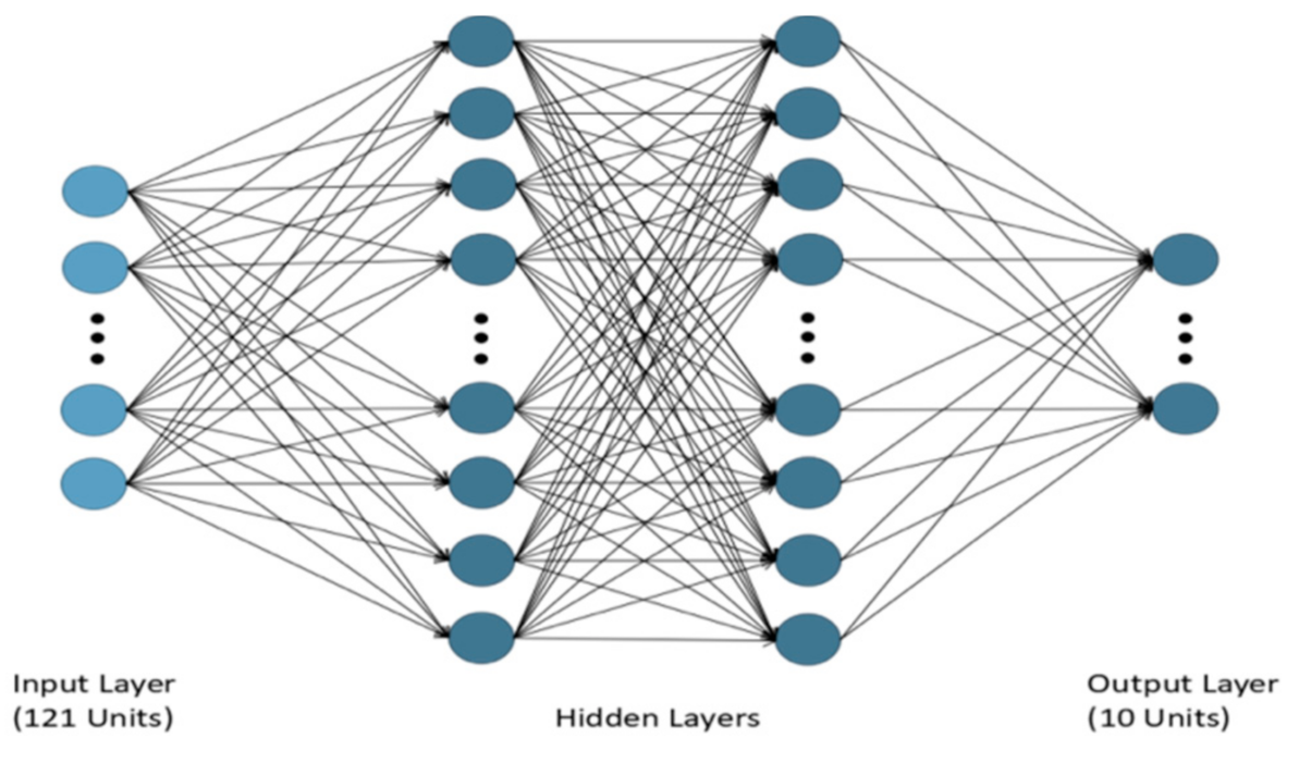
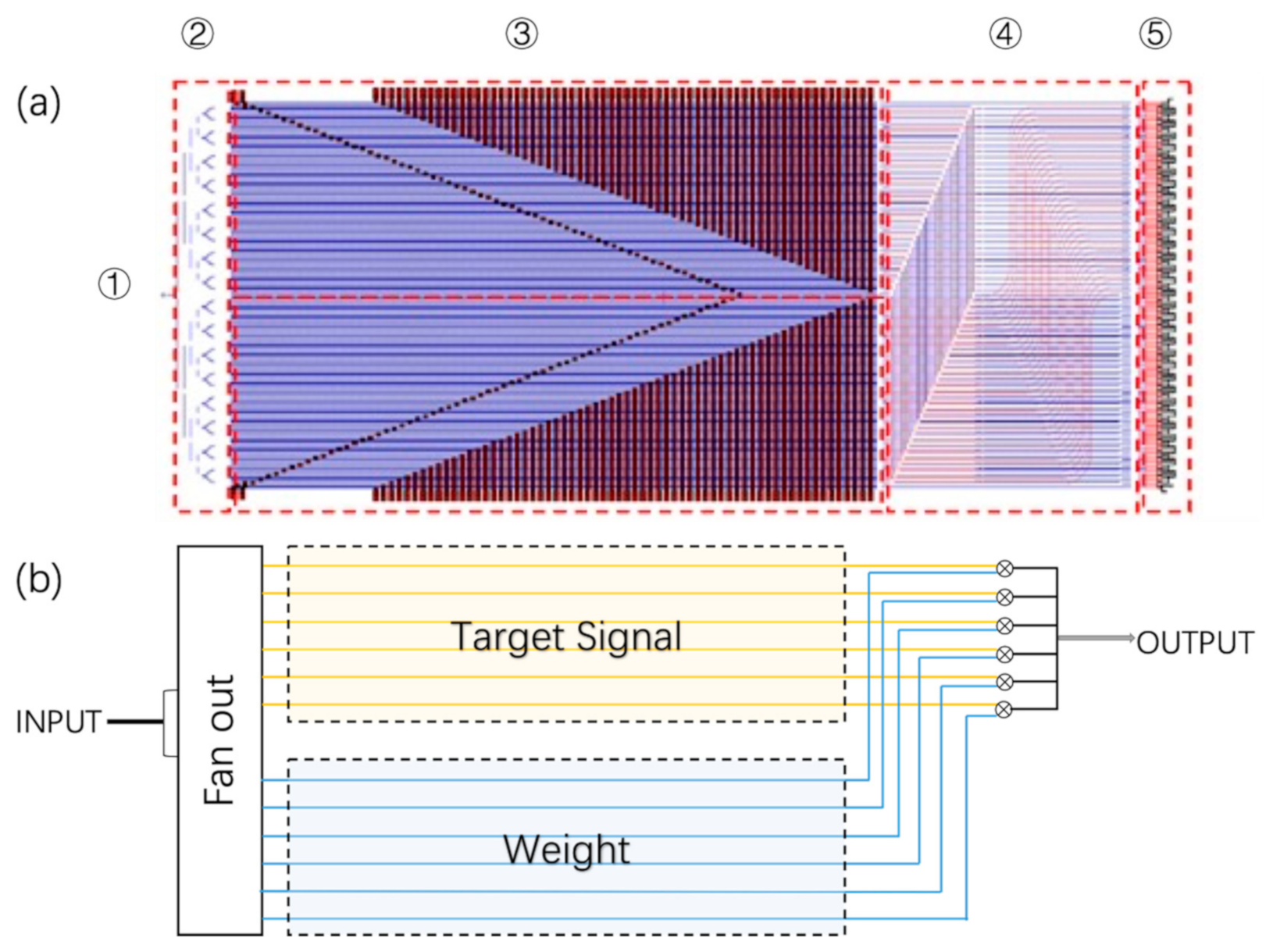
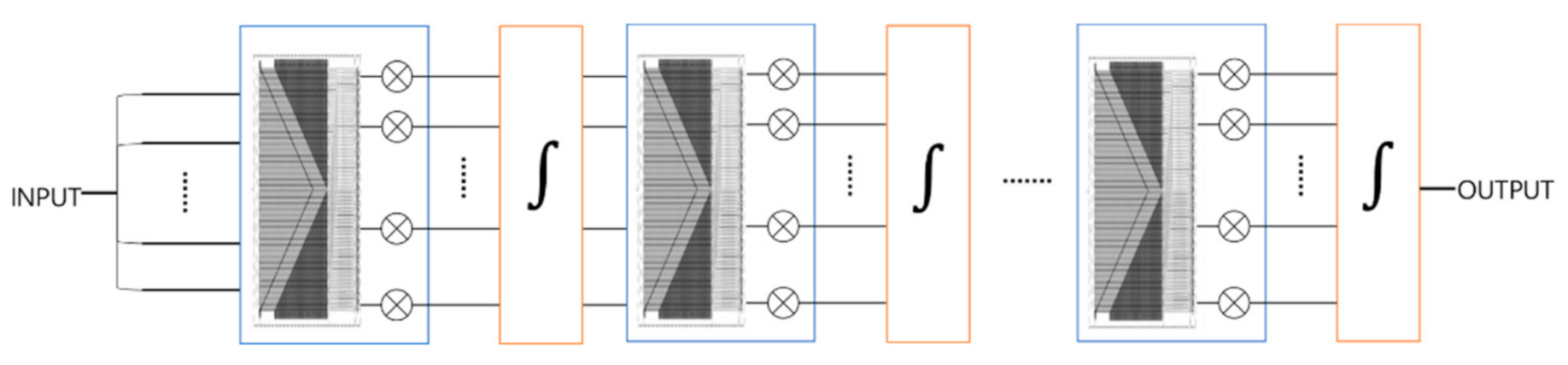
2.1. Neural Networks and ONNs
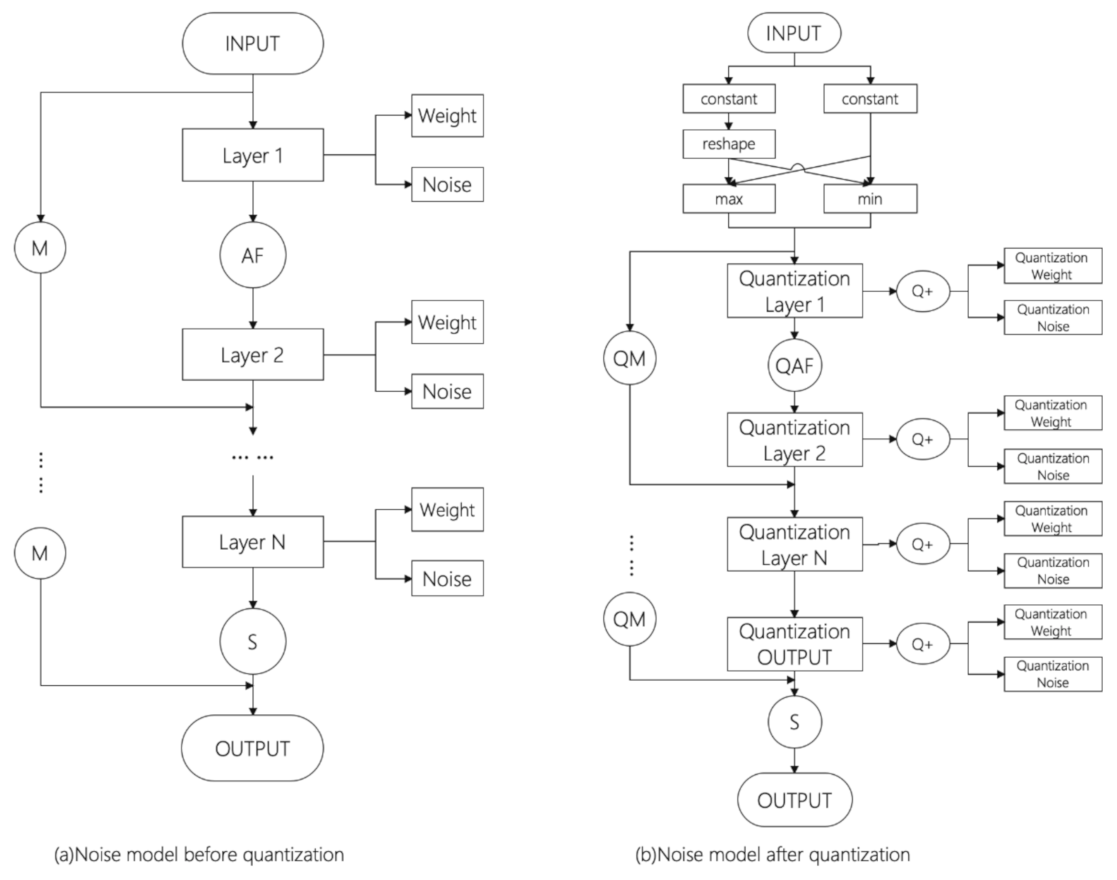
2.2. Noise
2.3. Quantization
3. Simulation and Results
3.1. Evaluation Criteria
3.2. Model Establishment
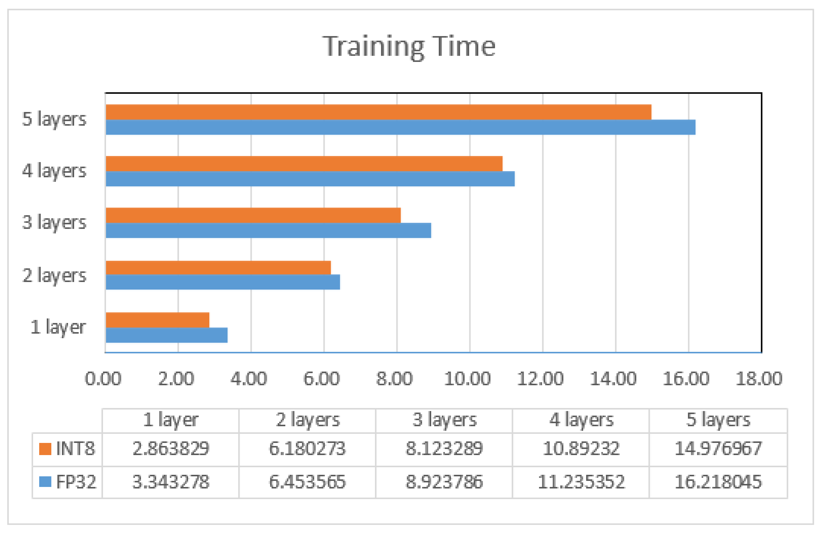
3.3. Model Training
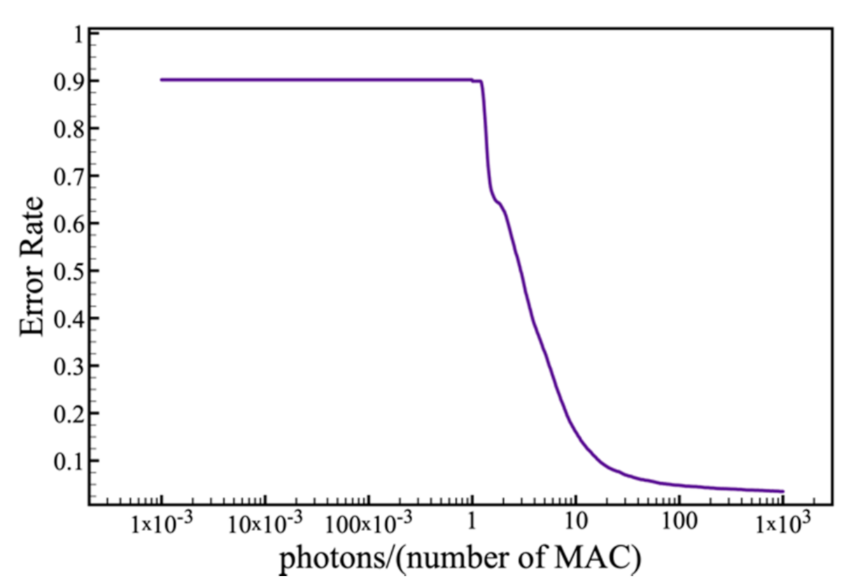
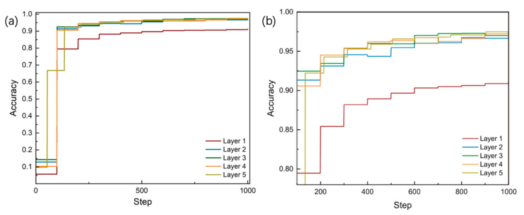
3.4. Noise
4. Conclusions
Author Contributions
Funding
Institutional Review Board Statement
Informed Consent Statement
Data Availability Statement
Conflicts of Interest
References
- Gallus, J. Fostering Public Good Contributions with Symbolic Awards: A Large-Scale Natural Field Experiment at Wikipedia. Manag. Sci. 2017, 63, 3999–4015. [Google Scholar] [CrossRef] [Green Version]
- Tkachenko, R.; Izonin, I.; Vitynskyi, P.; Lotoshynska, N.; Pavlyuk, O. Development of the Non-Iterative Supervised Learning Predictor Based on the Ito Decomposition and SGTM Neural-Like Structure for Managing Medical Insurance Costs. Data 2018, 3, 46. [Google Scholar] [CrossRef] [Green Version]
- Shen, Y.; Harris, N.C.; Skirlo, S.; Prabhu, M.; Baehr-Jones, T.; Hochberg, M.; Sun, X.; Zhao, S.; LaRochelle, H.; Englund, D.; et al. Deep learning with coherent nanophotonic circuits. Nat. Photon. 2017, 11, 441–446. [Google Scholar] [CrossRef]
- Hamerly, R.; Bernstein, L.; Sludds, A.; Soljačić, M.; Englund, D. Large-Scale Optical Neural Networks Based on Photoelectric Multiplication. Phys. Rev. X 2019, 9, 021032. [Google Scholar] [CrossRef] [Green Version]
- Zhang, H.; Gu, M.; Jiang, X.D.; Thompson, J.; Cai, H.; Paesani, S.; Santagati, R.; Laing, A.; Zhang, Y.; Yung, M.H.; et al. An optical neural chip for implementing complex-valued neural network. Nat. Commun. 2021, 12, 1–11. [Google Scholar]
- Anika, N.J.; Mia, B. Design and analysis of guided modes in photonic waveguides using optical neural network. Optik 2021, 228, 165785. [Google Scholar] [CrossRef]
- Hughes, T.W.; Minkov, M.; Shi, Y.; Fan, S. Training of photonic neural networks through in situ backpropagation and gradient measurement. Optica 2018, 5, 864–871. [Google Scholar] [CrossRef]
- Williamson, I.A.D.; Hughes, T.W.; Minkov, M.; Bartlett, B.; Pai, S.; Fan, S. Reprogrammable Electro-Optic Nonlinear Activation Functions for Optical Neural Networks. IEEE J. Sel. Top. Quantum Electron. 2020, 26, 1–12. [Google Scholar] [CrossRef] [Green Version]
- Pai, S.; Bartlett, B.; Solgaard, O.; Miller, D.A.B. Matrix Optimization on Universal Unitary Photonic Devices. Phys. Rev. Appl. 2019, 11, 064044. [Google Scholar] [CrossRef] [Green Version]
- Gu, J.; Zhao, Z.; Feng, C.; Zhu, H.; Chen, R.T.; Pan, D.Z. ROQ: A noise-aware quantization scheme towards robust optical neural networks with low-bit controls. In Proceedings of the Design, Automation & Test in Europe Conference & Exhibition (DATE), Grenoble, France, 9–13 March 2020; IEEE: Piscataway, NJ, USA, 2020. [Google Scholar]
- Harris, N.C.; Ma, Y.; Mower, J.; Baehr-Jones, T.; Englund, D.; Hochberg, M.; Galland, C. Efficient, compact and low loss thermo-optic phase shifter in silicon. Opt. Express 2014, 22, 10487–10493. [Google Scholar] [CrossRef] [PubMed] [Green Version]
- Fang, M.Y.-S.; Manipatruni, S.; Wierzynski, C.; Khosrowshahi, A.; Deweese, M.R. Design of optical neural networks with component imprecisions. Opt. Express 2019, 27, 14009–14029. [Google Scholar] [CrossRef] [PubMed] [Green Version]
- Tait, A.N.; Nahmias, M.A.; Shastri, B.J.; Prucnal, P.R. Broadcast and Weight: An Integrated Network for Scalable Photonic Spike Processing. J. Light. Technol. 2014, 32, 4029–4041. [Google Scholar] [CrossRef]
- Slussarenko, S.; Weston, M.M.; Chrzanowski, H.M.; Shalm, L.K.; Verma, V.B.; Nam, S.W.; Pryde, G.J. Unconditional violation of the shot-noise limit in photonic quantum metrology. Nat. Photon. 2017, 11, 700–703. [Google Scholar] [CrossRef] [Green Version]
- Zhang, D.; Wang, P.; Luo, G.; Bi, Y.; Zhang, Y.; Yi, J.; Su, Y.; Zhang, Y.; Pan, J. Design of a Silicon-based Optical Neural Network. In Proceedings of the 2nd International Conference on Mathematics, Modeling and Simulation Technologies and Applications (MMSTA 2019), Xiamen, China, 27–28 October 2019; Atlantis Press: Dordrecht, The Netherlands, 2019. [Google Scholar]
- Hsu, K.-Y.; Li, H.-Y.; Psaltis, D. Holographic implementation of a fully connected neural network. Proc. IEEE 1990, 78, 1637–1645. [Google Scholar] [CrossRef]
- The Dataset MNIST. Available online: http://yann.lecun.com/exdb/mnist/ (accessed on 12 April 2021).
- Hinton, G.; Oriol, V.; Dean, J. Distilling the knowledge in a neural network. arXiv 2015, arXiv:1503.02531. [Google Scholar]
- Song, Q.; Zhao, Z.; Liu, Y. Stability analysis of complex-valued neural networks with probabilistic time-varying delays. Neurocomputing 2015, 159, 96–104. [Google Scholar] [CrossRef]
- Jacob, B.; Kligys, S.; Chen, B.; Zhu, M.; Tang, M.; Howard, A.; Adam, H.; Kalenichenko, D. Quantization and training of neural networks for efficient integer-arithmetic-only inference. In Proceedings of the IEEE Conference on Computer Vision and Pattern Recognition, Salt Lake City, UT, USA, 18–23 June 2018. [Google Scholar]
- Zhou, S.; Wu, Y.; Ni, Z.; Zhou, X.; Wen, H.; Zou, Y. Dorefa-net: Training low bitwidth convolutional neural networks with low bitwidth gradients. arXiv 2016, arXiv:1606.06160. [Google Scholar]
- Moren, K.; Goehringer, D. A framework for accelerating local feature extraction with OpenCL on multi-core CPUs and co-processors. J. Real-Time Image Process. 2019, 16, 901–918. [Google Scholar] [CrossRef]
- Wu, J.; Leng, C.; Wang, Y.; Hu, Q.; Cheng, J. Quantized Convolutional Neural Networks for Mobile Devices. In Proceedings of the IEEE Conference on Computer Vision and Pattern Recognition (CVPR), Las Vegas, NV, USA, 27–30 June 2016; IEEE: Piscataway, NJ, USA, 2016. [Google Scholar]
- Dettmers, T. 8-bit approximations for parallelism in deep learning. arXiv 2015, arXiv:1511.04561. [Google Scholar]
- Gupta, S.; Agrawal, A.; Gopalakrishnan, K.; Narayanan, P. Deep learning with limited numerical precision. In Proceedings of the International Conference on Machine Learning, Lille, France, 6–11 July 2015. [Google Scholar]


| Number of Layers | FP32 | INT8 | Total Consumption |
|---|---|---|---|
| Layer 1 | 0.7903 | 0.7791 | |
| Layer 2 | 0.9371 | 0.9366 | |
| Layer 3 | 0.9417 | 0.9386 | |
| Layer 4 | 0.9551 | 0.9501 | |
| Layer 5 | 0.9635 | 0.9602 |
| Number of Layers | FP32 | INT8 |
|---|---|---|
| Layer 1 | 0.9117 | 0.9038 |
| Layer 2 | 0.9663 | 0.9627 |
| Layer 3 | 0.9678 | 0.9675 |
| Layer 4 | 0.9727 | 0.9721 |
| Layer 5 | 0.9749 | 0.9743 |
Publisher’s Note: MDPI stays neutral with regard to jurisdictional claims in published maps and institutional affiliations. |
© 2021 by the authors. Licensee MDPI, Basel, Switzerland. This article is an open access article distributed under the terms and conditions of the Creative Commons Attribution (CC BY) license (https://creativecommons.org/licenses/by/4.0/).
Share and Cite
Zhang, D.; Zhang, Y.; Zhang, Y.; Su, Y.; Yi, J.; Wang, P.; Wang, R.; Luo, G.; Zhou, X.; Pan, J. Training and Inference of Optical Neural Networks with Noise and Low-Bits Control. Appl. Sci. 2021, 11, 3692. https://0-doi-org.brum.beds.ac.uk/10.3390/app11083692
Zhang D, Zhang Y, Zhang Y, Su Y, Yi J, Wang P, Wang R, Luo G, Zhou X, Pan J. Training and Inference of Optical Neural Networks with Noise and Low-Bits Control. Applied Sciences. 2021; 11(8):3692. https://0-doi-org.brum.beds.ac.uk/10.3390/app11083692
Chicago/Turabian StyleZhang, Danni, Yejin Zhang, Ye Zhang, Yanmei Su, Junkai Yi, Pengfei Wang, Ruiting Wang, Guangzhen Luo, Xuliang Zhou, and Jiaoqing Pan. 2021. "Training and Inference of Optical Neural Networks with Noise and Low-Bits Control" Applied Sciences 11, no. 8: 3692. https://0-doi-org.brum.beds.ac.uk/10.3390/app11083692