Noise Reduction Effect of Superhydrophobic Surfaces with Streamwise Strip of Channel Flow


1
Acoustic Science and Technology Laboratory, Harbin Engineering University, Harbin 150001, China
2
Key Laboratory of Marine Information Acquisition and Security, Ministry of Industry and Information Technology, Harbin Engineering University, Harbin 150001, China
3
College of Underwater Acoustic Engineering, Harbin Engineering University, Harbin 150001, China
*
Author to whom correspondence should be addressed.
Appl. Sci. 2021, 11(9), 3869; https://0-doi-org.brum.beds.ac.uk/10.3390/app11093869
Submission received: 8 April 2021
/
Revised: 22 April 2021
/
Accepted: 23 April 2021
/
Published: 25 April 2021
(This article belongs to the Special Issue Recent Advances in Flow-Induced Noise)
Abstract
:Superhydrophobic surface is a promising technology, but the effect of superhydrophobic surface on flow noise is still unclear. Therefore, we used alternating free-slip and no-slip boundary conditions to study the flow noise of superhydrophobic channel flows with streamwise strips. The numerical calculations of the flow and the sound field have been carried out by the methods of large eddy simulation (LES) and Lighthill analogy, respectively. Under a constant pressure gradient (CPG) condition, the average Reynolds number and the friction Reynolds number are approximately set to 4200 and 180, respectively. The influence on noise of different gas fractions (GF) and strip number in a spanwise period on channel flow have been studied. Our results show that the superhydrophobic surface has noise reduction effect in some cases. Under CPG conditions, the increase in GF increases the bulk velocity and weakens the noise reduction effect. Otherwise, the increase in strip number enhances the lateral energy exchange of the superhydrophobic surface, and results in more transverse vortices and attenuates the noise reduction effect. In our results, the best noise reduction effect is obtained as 10.7 dB under the scenario of the strip number is 4 and GF is 0.5. The best drag reduction effect is 32%, and the result is obtained under the scenario of GF is 0.8 and strip number is 1. In summary, the choice of GF and the number of strips is comprehensively considered to guarantee the performance of drag reduction and noise reduction in this work.
1. Introduction and Principle Headings
Hydrodynamic noise is one of three major noises of underwater vehicles, and studying and controlling it are important [1,2,3,4,5,6,7,8,9,10]. The hydrodynamic noise is mainly caused by the velocity and pressure fluctuation in turbulent flow. Especially at medium and high velocity, hydrodynamic noise has become the main factor to affect the self-noise of sonar platforms on underwater vehicles. The study and suppression of the hydrodynamic noise on the surface of the underwater vehicle dome and towing array [11,12,13,14,15,16] attach great importance to increase the detection range of the sonar platform and improve the signal-to-noise ratio. Traditionally, the acoustic performance of underwater vehicles is considered from linear optimization, material optimization, and structural optimization. These three traditional methods are not only difficult to implement, but also to balance the mechanical performance and the noise performance at the same time. Conversely, the superhydrophobic surface does not change the macrostructure of the sonar array platform, causes little damage to the shape of the underwater vehicles, and does not increase the wet area of the underwater vehicles.
Superhydrophobic surfaces is an emerging technology that combines low surface energy chemical properties with microstructures physical properties. The discovery of superhydrophobic surfaces are inspired by the water droplet on lotus leaf. Superhydrophobicity can only be obtained if the Cassie [17] state is maintained, and this property can bring some benefits, such as drag reduction, self-cleaning and anti-fog. Microstructures on the surfaces can capture the air and transfer the liquid-solid contact to liquid-air contact, which will cause a slip velocity and change the near-wall flow regime. Scholars have studied the flow regimes changes on superhydrophobic surfaces with different parameters through experiments, simulations, and theoretical analysis.
In theoretical analysis and simulation, a steady superhydrophobic surface always equivalent to free-slip or fixed slip length boundary condition. Philip [18] used the free-slip hypothesis to analyze the flow regime of Stokes flow and obtained the functions of velocity distribution on superhydrophobic surfaces with different parameters. His results played a guiding role for subsequent research. Most studies on superhydrophobic surfaces are based on channel flow. The upper and lower plates in channel are set to different boundary condition to simulate the superhydrophobic surfaces. In laminar flow, the slip velocity and slip length of the superhydrophobic surface can reduce the flow resistance, and a higher proportion of the free-slip surface corresponds to a greater slip length formed by the superhydrophobic surface. As a result, the drag reduction effect of the superhydrophobic surfaces is associated with the proportion of free-slip boundary. The height of channel and the shape of microstructures also influence the drag reduction effect. The streamwise microstructures generally have better drag reduction than spanwise microstructures. The spanwise slip velocity generated by the spanwise microstructure can even increase the flow resistance. Micro-post can generate higher slip velocity than micro-grooves, but the gas-liquid interface is easily to destroyed on micro-post [19,20,21,22,23]. From the literature listed above, we concluded that the streamwise strips have a better effect on drag reduction. Hence, we chosen the streamwise strip as the object to study the noise reduction effect.
In turbulent flow, the research objects on superhydrophobic surface flow are not only slip velocity and slip length, but also the vortex, Reynolds stress, and other parameters of boundary layer caused by the velocity difference between the free-slip and the no-slip surfaces. In the study of flow regime on superhydrophobic surfaces, the turbulent flow on superhydrophobic surfaces have obvious changes compared with ordinary smooth surfaces, and the influence of these changes on hydrodynamic noise is still unclear.
In turbulent flow, Min and Kim [24] studied the influence of streamwise and spanwise slip boundary conditions on turbulent flow through direct numerical simulation. Their results proved that streamwise slip length can effectively weaken the turbulence intensity and vortex, while the spanwise slip length increases the flow resistance. Thereafter, the flow under different microstructures’ type, size, spacing, and air-water contact area fraction on superhydrophobic surfaces under different Reynolds numbers have been studied. They found that the increase in the microstructure spacing, the decrease in the proportion of no-slip surface, and the change in the number of microstructures cause significant changes in the Reynolds stress distribution and significantly weaken the flow resistance. Otherwise, micro-posts with large spacing have better drag reduction effects than micro-riblets, but the turbulent structures have a slight difference. Angular microstructures will reduce the secondary flow and turbulent sweeping up and down movement. As the increase in Reynolds number reduces the drag reduction effect, the effective slip length of the wall still increases [22,25,26,27].
S. Turk [28] verified that constant pressure gradient (CPG) in the study of the turbulent structure on superhydrophobic surfaces is more profit than constant flow rate (CFR). They analyzed the flow regime changes on superhydrophobic surfaces from different turbulent parameters, and proposed the generation and distribution of secondary flow on superhydrophobic surfaces. J. Seo [29] studied on a larger size scale of microstructure and selected microstructures of micro-posts and micro-ridges. The results showed that the influence of size on the micro-posts is more obvious than that on micro-ridges. Friction Reynolds number changes slightly affect the flow structure, while the size of microstructures and Weber number are important factors of the turbulent structure. CT Faithal [30] separated the influence of the slip length and the surface topography on superhydrophobic surfaces, and proved that the turbulent structure changes are mainly affected by the surface topography. Amirreza [31,32] simulated and analyzed the flow of superhydrophobic surfaces under different gas-liquid contact surface angles at different Reynolds numbers. Im [33] compared channel flow and pipe flow under similar boundary conditions. They found that the lateral slip in the superhydrophobic pipe is relatively large and certain vorticities has been formed. Furtherly, the vorticities will generate secondary flow and weaken the energy transport of convective vortices. Roberta [34] used equivalent boundary conditions to analyze the vorticities, Reynolds stress, and the reasons for velocity increment in the pipeline. Therefore, in the analysis of flow noise, the secondary flow and the parameter changes of microstructures probably play an important role in the analysis of flow noise.
In addition to numerical simulations, many experimental studies are conducted on the flow regimes of superhydrophobic surfaces under turbulent flow. Robert J. Daniello [35] first studied the flow on superhydrophobic surfaces with microstructures. The results are consistent with Min and Kim’s DNS results and the theoretical analysis of Koji Fukugata [36]. Therefore, the flow changes caused by the increase in depth and space improved the drag reduction effect of the superhydrophobic surface under a given Reynolds number. Otherwise, when the thickness of the viscous bottom layer is close to microstructures, the drag reduction effect will be significantly increased. These results verify the possibility of using superhydrophobic surfaces in underwater vehicle. Thereafter, velocity distribution, lift and drag force characteristics, and changes in the wettability of superhydrophobic surfaces under different Reynolds numbers and pressure are studied. The results indicated that if the near-wall turbulent flow is changed, a certain drag reduction effect can be obtained, as long as the gas can be maintained in the microstructures regardless under a random surface or a regular surface [37,38,39,40].
Overall, we found that the superhydrophobic surface can change the turbulent flow regimes, affect the peak value of Reynolds stress, and change the thickness of the boundary layer. Moreover, in the study of different microstructures, the streamwise microstructure can weaken the turbulence intensity and reduce the number of streamwise vorticities near the wall. The space and size of the streamwise microstructures also directly affect the formation of vortex structure near the wall. If the space is larger and the surface solid fraction is smaller, the turbulent stress will be smaller. Although the listed works have studied the turbulent flow of superhydrophobic surfaces, the ultimate goal is attributed to drag reduction effect. The effect of superhydrophobic surface with different parameters on hydrodynamic noise still requires systematic research. Therefore, we focus on the study of noise reduction effect in a channel flow with streamwise strips and find the connection between drag reduction and noise reduction. In Section 2, the simulation methods are briefly introduced, and the accuracy is also verified. In Section 3, the results are discussed from different aspects. In Section 4, we concluded the relationship between noise reduction effect and streamwise strips parameters.
2. Problem Formulation and Simulation Methods
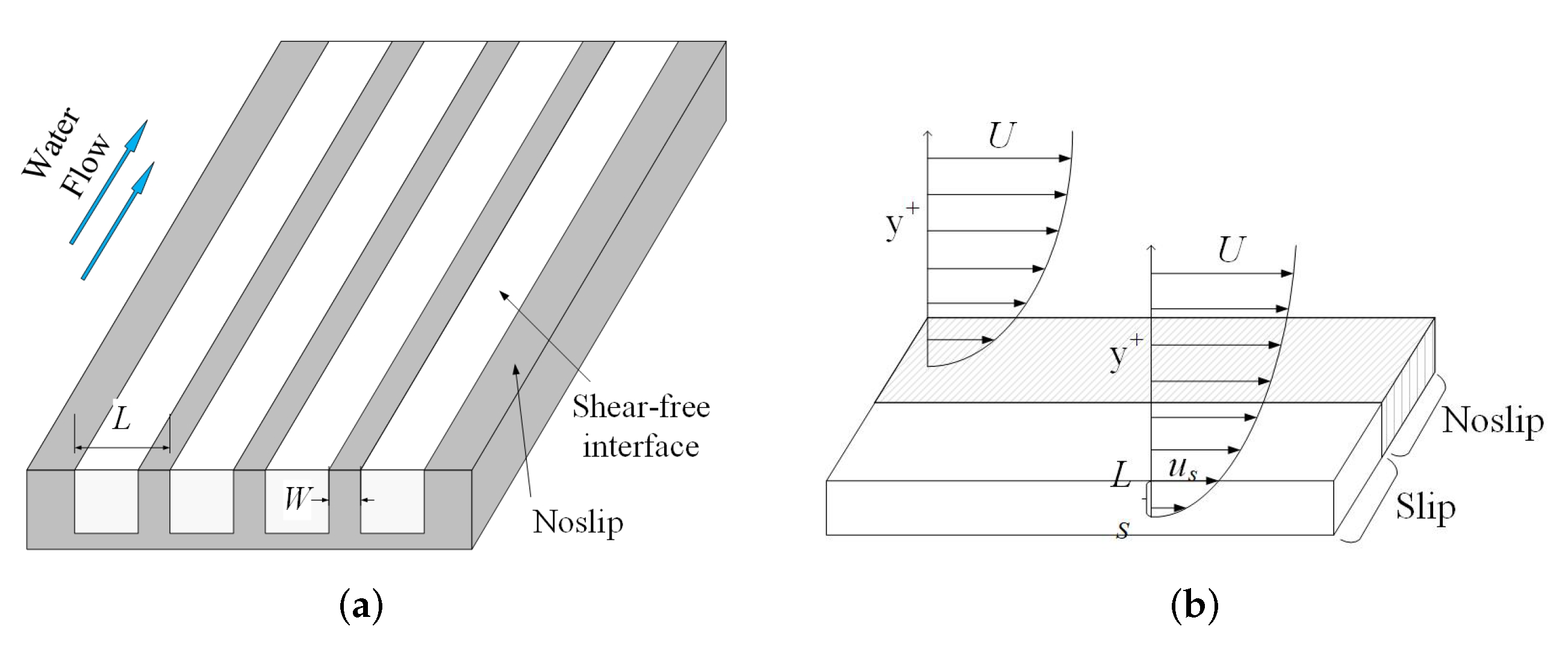
We studied a fully developed turbulent channel flow. The top-wall and bottom-wall are no-slip boundary and superhydrophobic surfaces, respectively. Superhydrophobic surfaces are streamwise strip composed of alternating no-slip and free-slip boundary conditions. The space of strip is W. The length of microstructure which contains a no-slip strip and a free-slip is L. The details are shown in Figure 1a.
The channel flow is governed by incompressible Navier–Stokes equation.
where is dynamic viscous and is density of water. We have simplified the boundary condition of superhydrophobic surfaces. Therefore, the liquid-solid interface and the liquid-air interface are equal to no-slip and free-slip boundary condition. The velocity distribution profiles of slip boundary are shown in Figure 1b, which satisfies the Navier slip equation.
where is slip velocity and is slip length. This simplified method is proven to be reliable. When the liquid-air interface deformation is negligible compared with the width of microstructures, the gas-liquid viscosity ratio is sufficiently small, and the depth is equal to the width of the microstructure. The reasonability of the hypothesis has been verified [25,28,29,41]. Although this assumption improves the drag reduction effect, the overall trend of Reynolds stress is still consistent in the prediction of turbulence characteristics. Therefore, the alternating boundary conditions of no-slip and free-slip have been used in this work to simulate superhydrophobic surfaces with streamwise strips. Through the change of the percentage of free-slip boundary conditions and the number of strips, the flow noise of superhydrophobic surfaces is calculated.
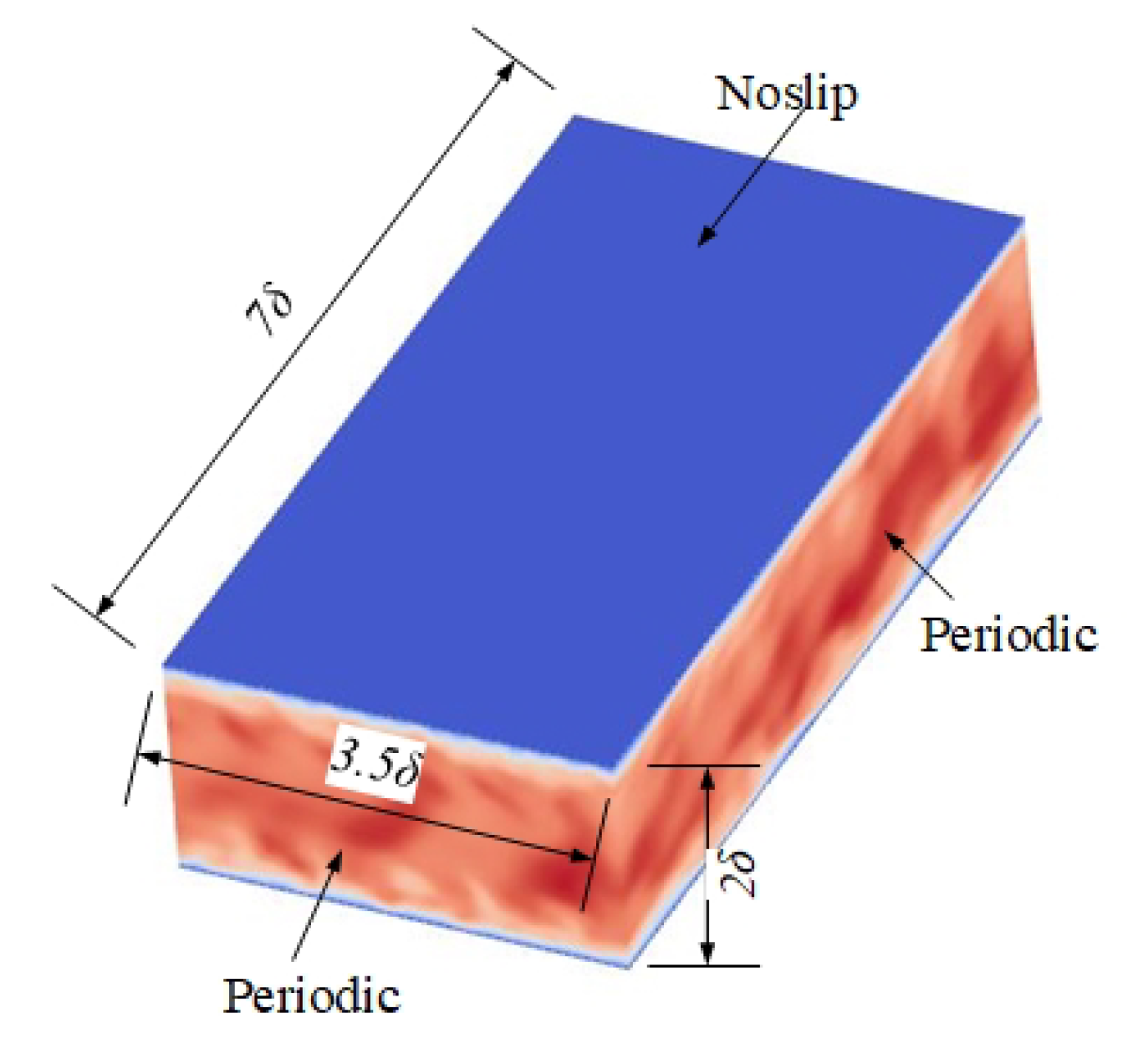
The size of flow field is set to at streamwise, wall-normal, and spanwise direction, respectively. Where is the half height of channel. The flow Reynolds number in this work is and the friction Reynolds number is , where is the velocity in channel centerline and is wall friction velocity. The flow region size is consistent with that of Min and Kim [24] to ensure the accuracy of simulation. The top boundary is no-slip wall and the bottom boundary is superhydrophobic surfaces with alternating strips. Other sides are periodic boundary. The flow is driven by CPG. At the initial time, we produced some random turbulence to help the flow to fully develop. The details are shown in Figure 2.
The large eddy simulation (LES) is a mathematical solved model for turbulence in computational fluid dynamics. This simulation method can achieve flow regimes more precisely than the Reynolds-averaged Navier–Stokes equations method. The vortices are the main cause of flow noise according to the vortex sound theory. Each variable in LES is divided into two parts by the filter function. For example, the transient variables is divided into and , which are referred to as the large- and the small-scale component, respectively.
where D refers to the flow field, is the spatial coordinate in the original flow area, x is the filtered spatial coordinate on the large-scale space, and is the filter function that determines the vortices scale. The filter function represented by the above-mentioned formula is applied into the Navier–Stokes and the continuity equations under transient conditions. The equation can be obtained as follows:
Equations (5) and (6) constitute the governing equations in the LES. The overscored variable in Equation (6) denotes the filtered field variable. is defined as follows,
where refers to the subgrid-scale stress, which embodies the effect of the small-scale vortex motion on the governing equations.
The simulation method is LES and the sub-grid stress model is Wall-Adapting Local Eddy-viscosity (WAlE) model. The space discretization method is central difference. The grid is Cartesian with uniform spacing in the streamwise and spanwise directions, and stretching in the wall-normal direction. The grids number of no-slip boundary channel flow is 150 × 60 × 80. Other scenarios are shown in Table 1.
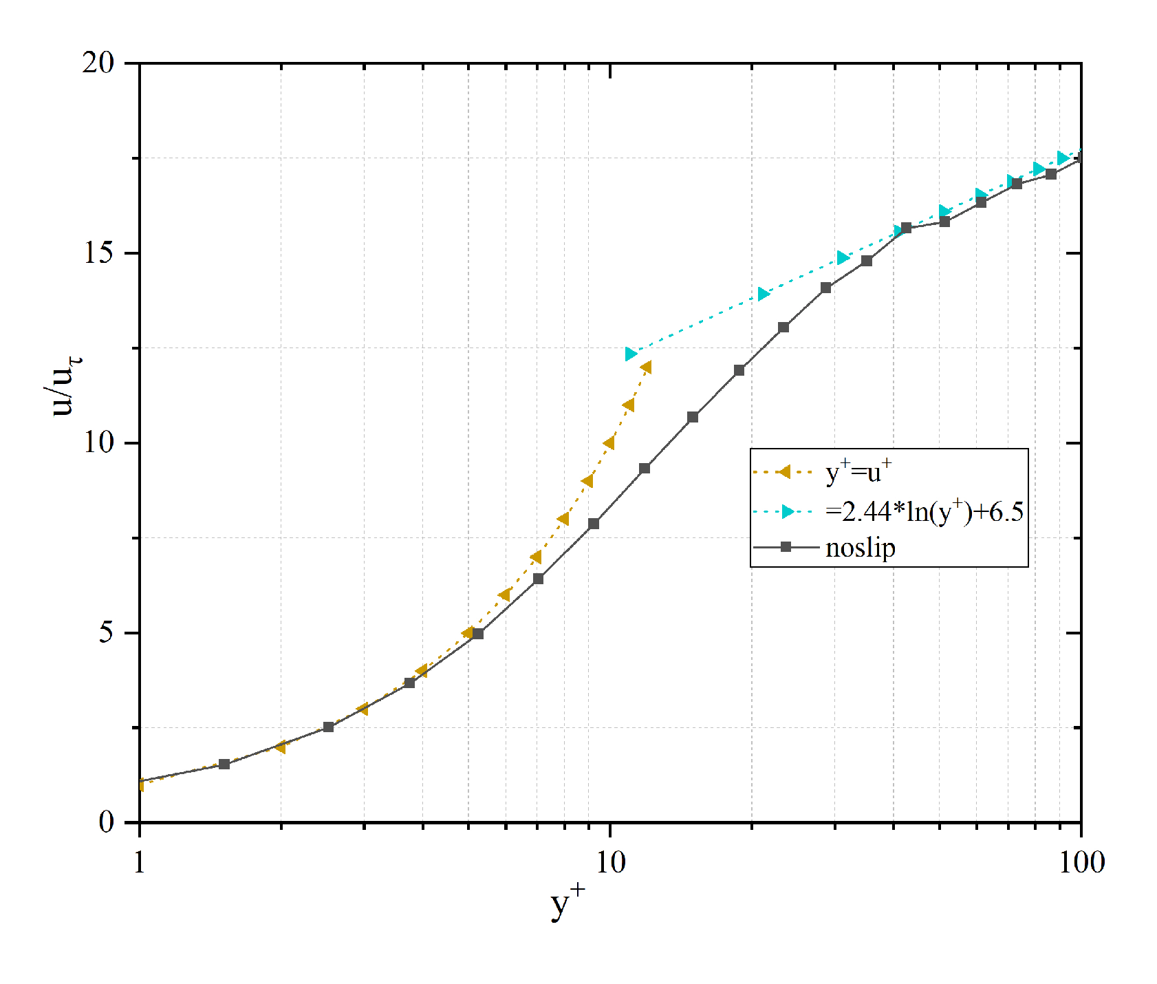
According to the LES, the is preferably less than 1 and the time step size need to satisfy the Courant-Friedrichs-Lewy (CFL) condition. Our time step size is and . The near-wall velocity profile is verified with the logarithmic law as shown in Figure 3. The grid and Wale constant independence verification are shown in Table 2. We have calculated the drag coefficients of four sets of grid. The results show that under the condition of , the change of grid number have a slight influence on the accuracy of flow field. Two experiential Wale constants have been chosen for verification and the results show that the Wale constant is appropriate.
The Lighthill analogy theory and hybrid numerical method [42,43] are used to calculate the flow noise of channel. The velocity variable in the flow simulation is extracted and used as source term in Equation (8).
where is sound speed. Q and F are mass and momentum changes in unit time, respectively. is Lighthill stress tensor. In particular, at the calculation of flow noise, the Lighthill stress tensor can simplified to .
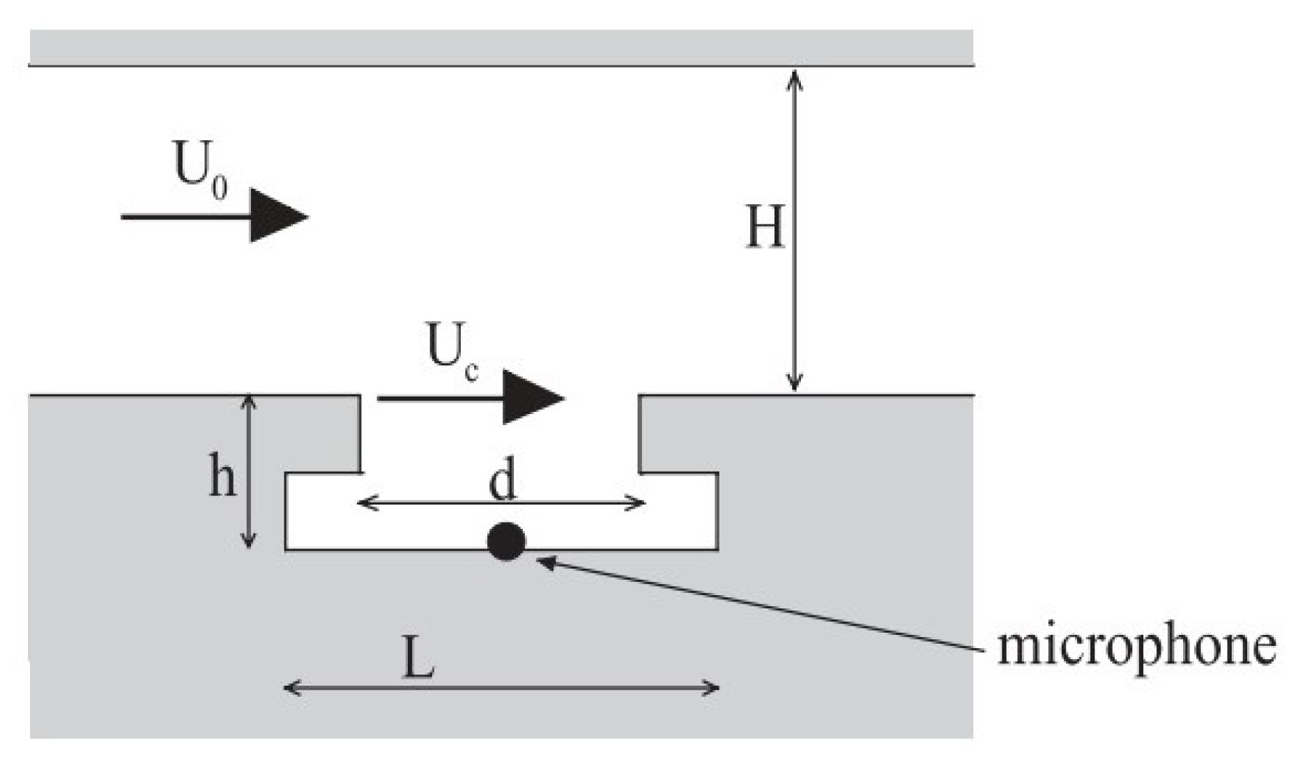
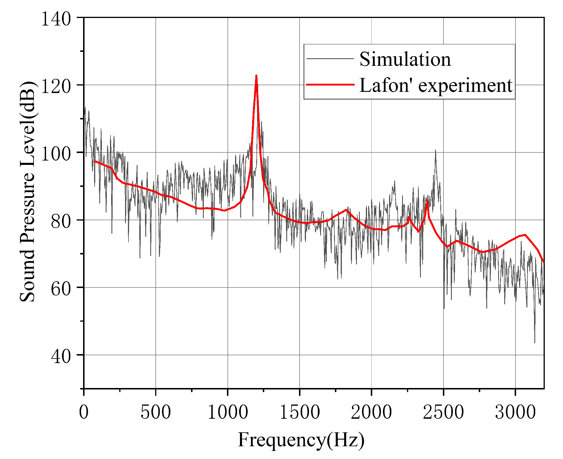
According to Equation (8), the flow field data can be used and interpolated to the sound calculation grids. Then, the Discrete Fourier Transform(DFT) is used to convert sound source from time domain to frequency domain. The finite element method is used to calculate the generation and propagation of flow noise. At the boundary, the infinite element method is used to simulate the no-reflection boundary. The accuracy of this method is proven by comparing with the flow noise experiment results of Lafon [44]. The flow noise of cavity in wind tunnel is tested, as shown in Figure 4 and Table 3.
Our simulation model is established and consistent with the experimental model. The sound pressure profile is calculated, as shown in Figure 5.
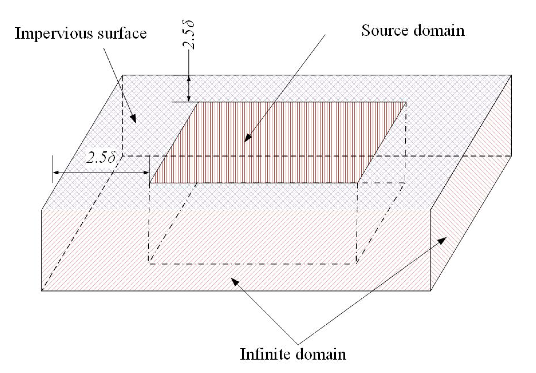
As shown in Figure 3 and Figure 5, our simulation results are greatly consistent with the experiment results. Therefore, the accuracy of the simulation method is proven. The same size and coordinates as the flow field should be maintained to accurately interpolate the flow field data into the sound field as a sound source. The sound calculation domain is shown in Figure 6.
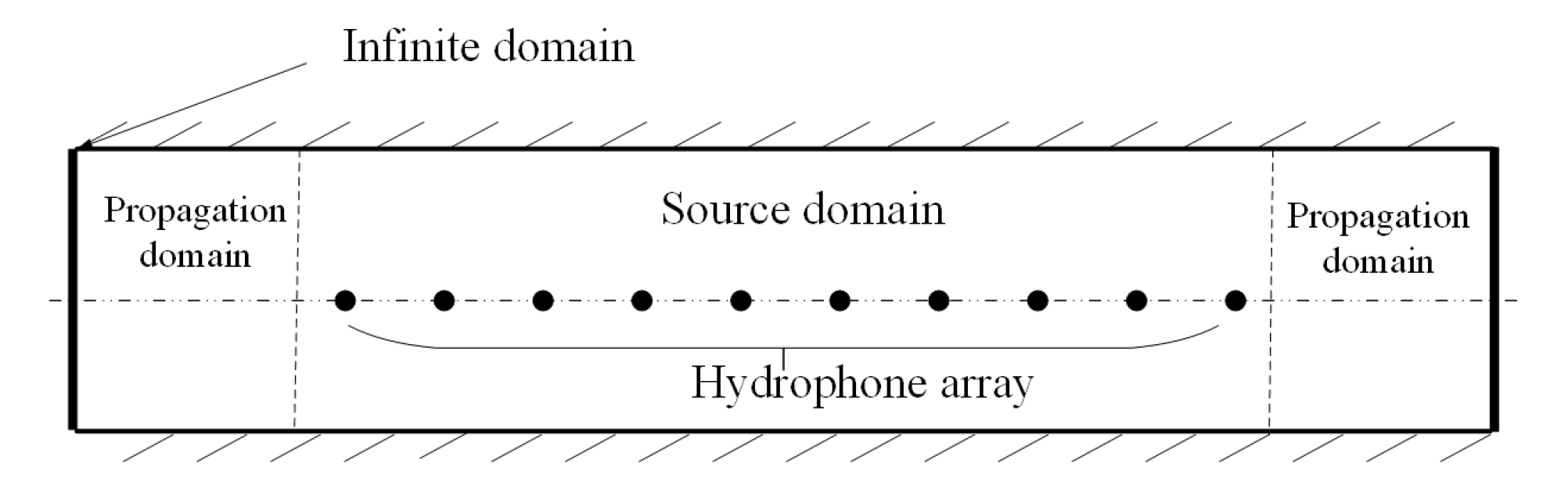
The size of center source area is , same as the flow field. The streamwise and spanwise directions of the sound source area extend as the sound propagation area. The upper and lower boundaries are impervious boundary, and the other boundary is infinite element domain to simulate no-reflection boundary. A total of 10 hydrophones are set in the sound field to monitor the sound pressure, to analyze the influence of the superhydrophobic surface on the flow noise. The hydrophone settings are shown in Figure 7.
3. Discussion
3.1. Turbulent Structures Changes on Superhydrophobic Surfaces
The hydrophones are arranged in the centerline of flow region where flow is stable to precisely collect sound pressure. Otherwise, the data of hydrophones are averaged. On consideration of the sampling theorem, the CFL condition, and the ram of computer, we set the frequency range to 100–30 kHz and the resolution to 100 Hz. The grid size of sound domain is one-sixth wavelength.
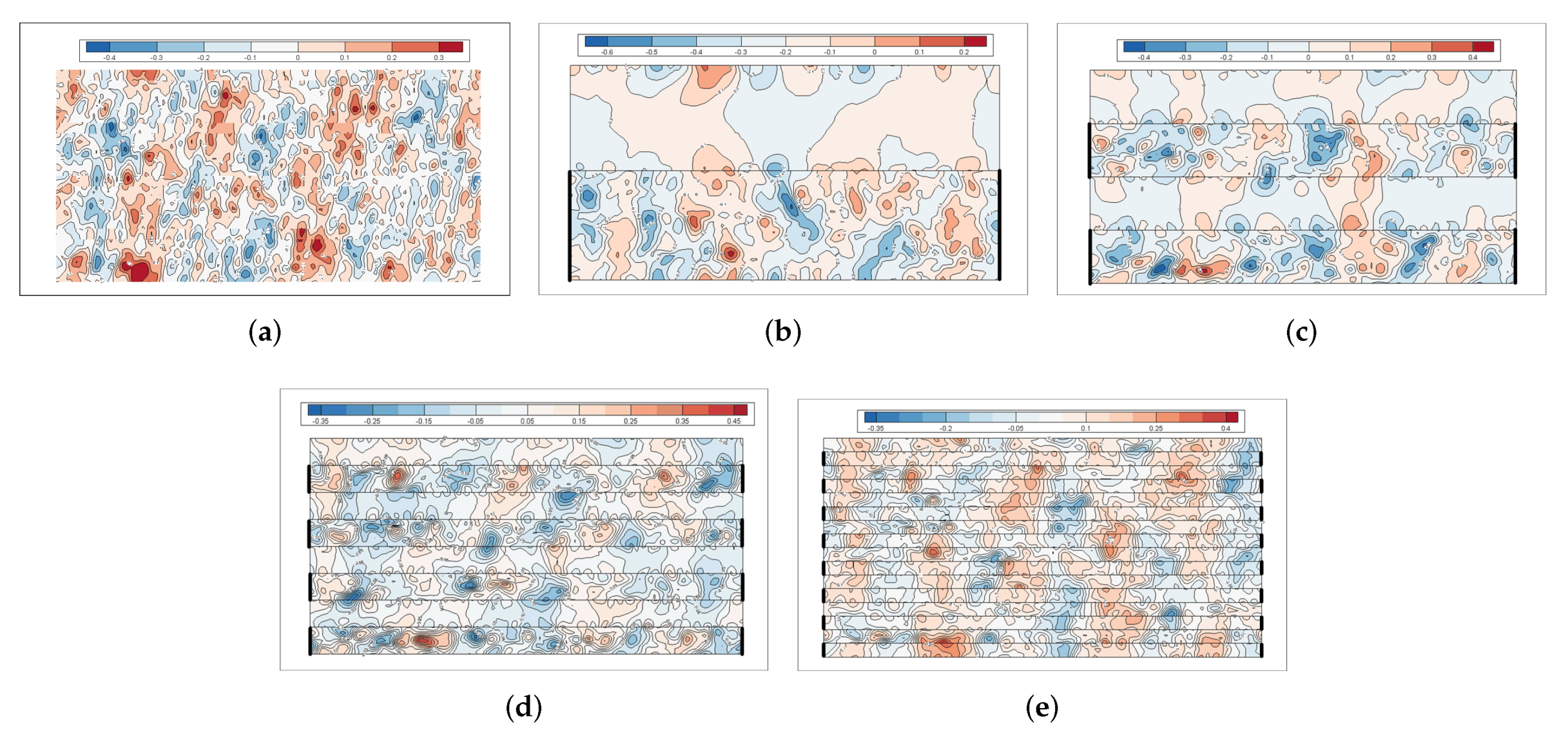
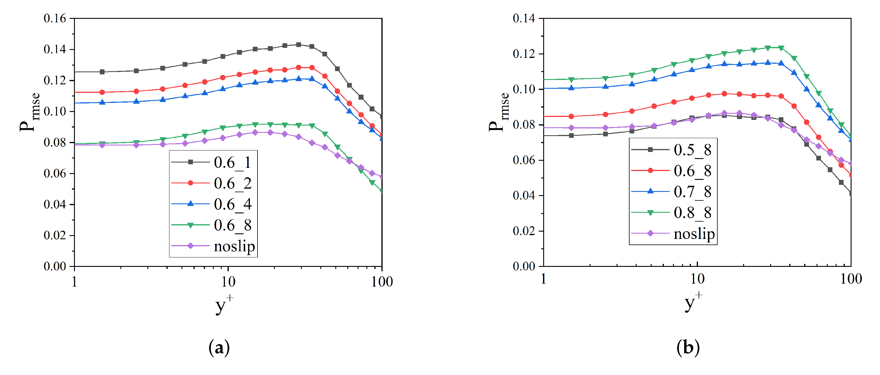
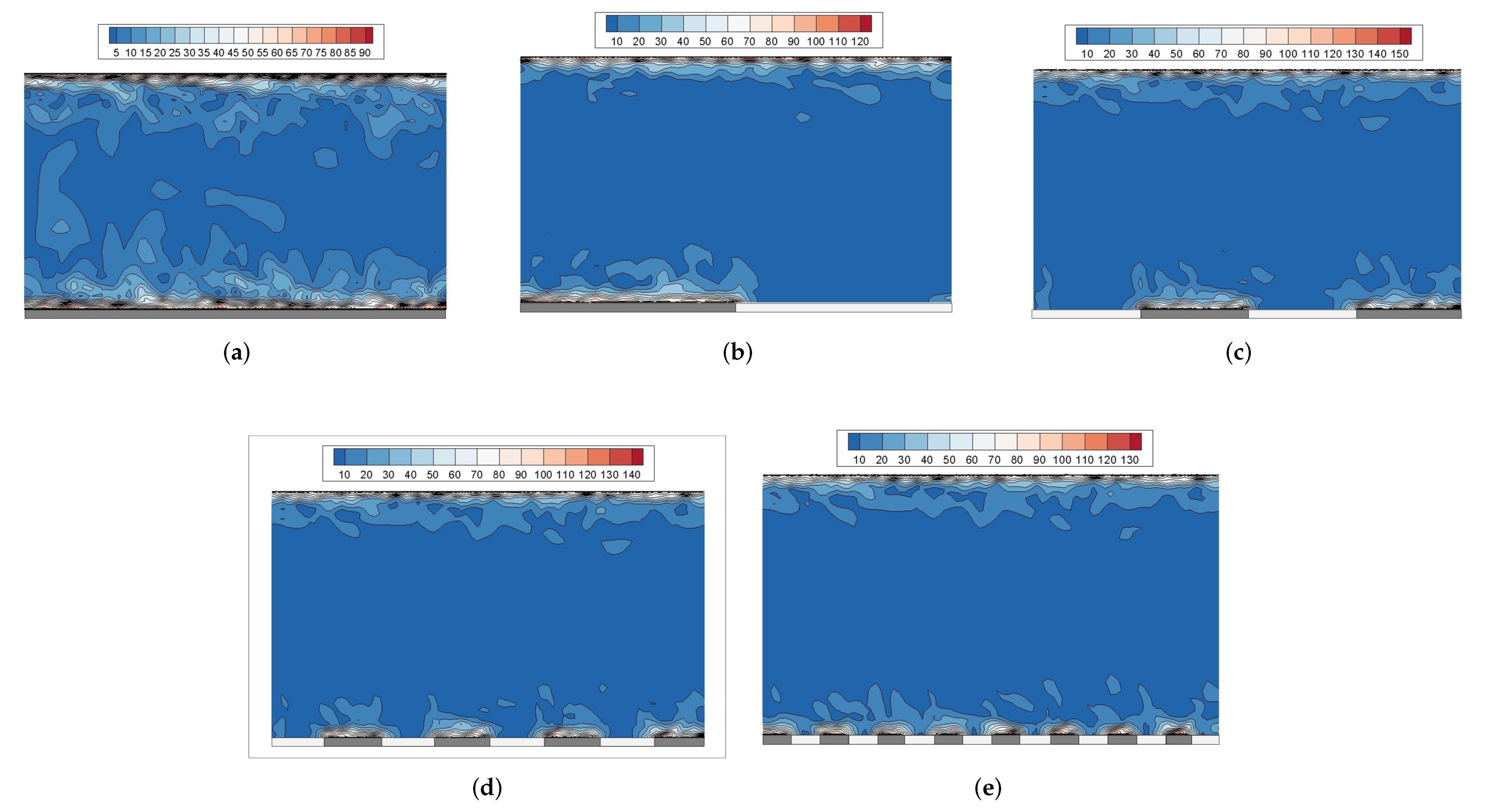
First, we compared the pressure changes of the superhydrophobic surface with alternating boundary conditions, as shown in Figure 8 and Figure 9. We fixed the fraction of the free-slip boundary as GF is 0.5 and compared the pressure distribution when the strip numbers are 1, 2, 4 and 8. In general, the pressure fluctuation of the no-slip surface is significantly higher than the superhydrophobic surface with strips at different numbers. The Figure 9 shows that the root mean square error of pressure at different strip number and GF. Similar to the distribution of boundary conditions, the pressure also exhibits alternating properties. When the number of strips is 2, a large range of low-pressure fluctuation areas are concentrated on the free-slip surface and multiple continuous high-pressure areas and low-pressure areas exist at the free-slip strips. Consequently, the pressure RMSE at has the largest value than others. As the number of strips increases, the frequent alternation of the free-slip and no-slip boundary results in an interactive influence. As a result, the fluctuating pressure is enhanced, and the range of continuous stable pressure areas decrease. When the number of strips is 8, the fluctuating pressure on superhydrophobic surface is close to the no-slip surface, and the noise reduction effect has been weakened.
The vorticity contours are shown in Figure 10, to further study the influence of flow regime changes on flow noise. According to vortex sound theory, the vortex is the voice of the fluid, we compared the vorticity of different strip numbers at . The vorticity contours of no-slip boundary channel is shown in Figure 10a. The vorticity is large at the overall flow field, especially at the near-wall region. However, the vorticity at free-slip boundary is 0, and the channel with free-slip boundary has a lower vorticity level. When the strip number is small, the vorticity distribution is more centralized. A clear boundary between the zero vorticity and the large vorticity is observed. The free-slip boundary and no-slip boundary have less mutual influence. The flow noise should have a lower level because of the large-scale lower vorticity distribution. However, when the strip number becomes large, the space between the free-slip and no-slip boundary becomes narrow. The interactive influence of free-slip and no-slip is obvious, and the lower vorticity part nearly disappears. Consequently, the flow noise level can be higher when the strip number is large.
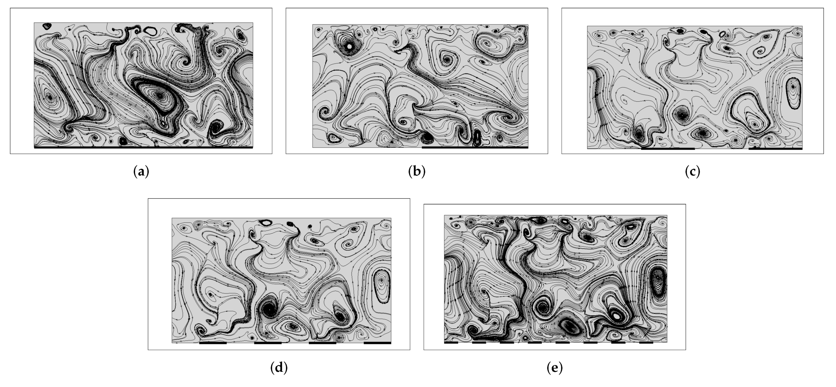
Note that the streamlines of velocity on cutplane are shown in Figure 11, we can draw the same conclusion. The channel with no-slip bottom boundary generates more lateral vortices. At the center of the flow field, the larger vortices can be found, which will generate higher low-frequency noise. Otherwise, small vortices are generated near the wall and increases the high-frequency components. As a result, the no-slip channel has a higher overall noise level. However, the number of lateral large vortices on the superhydrophobic surfaces with is significantly reduced, while the number of small vortices near the wall does not increase significantly. Therefore, the flow noise level must be lower. As the number of strips increases, more vortices will be generated with a size close to the strip width on the bottom and significantly affect the flow noise at some certain frequencies.
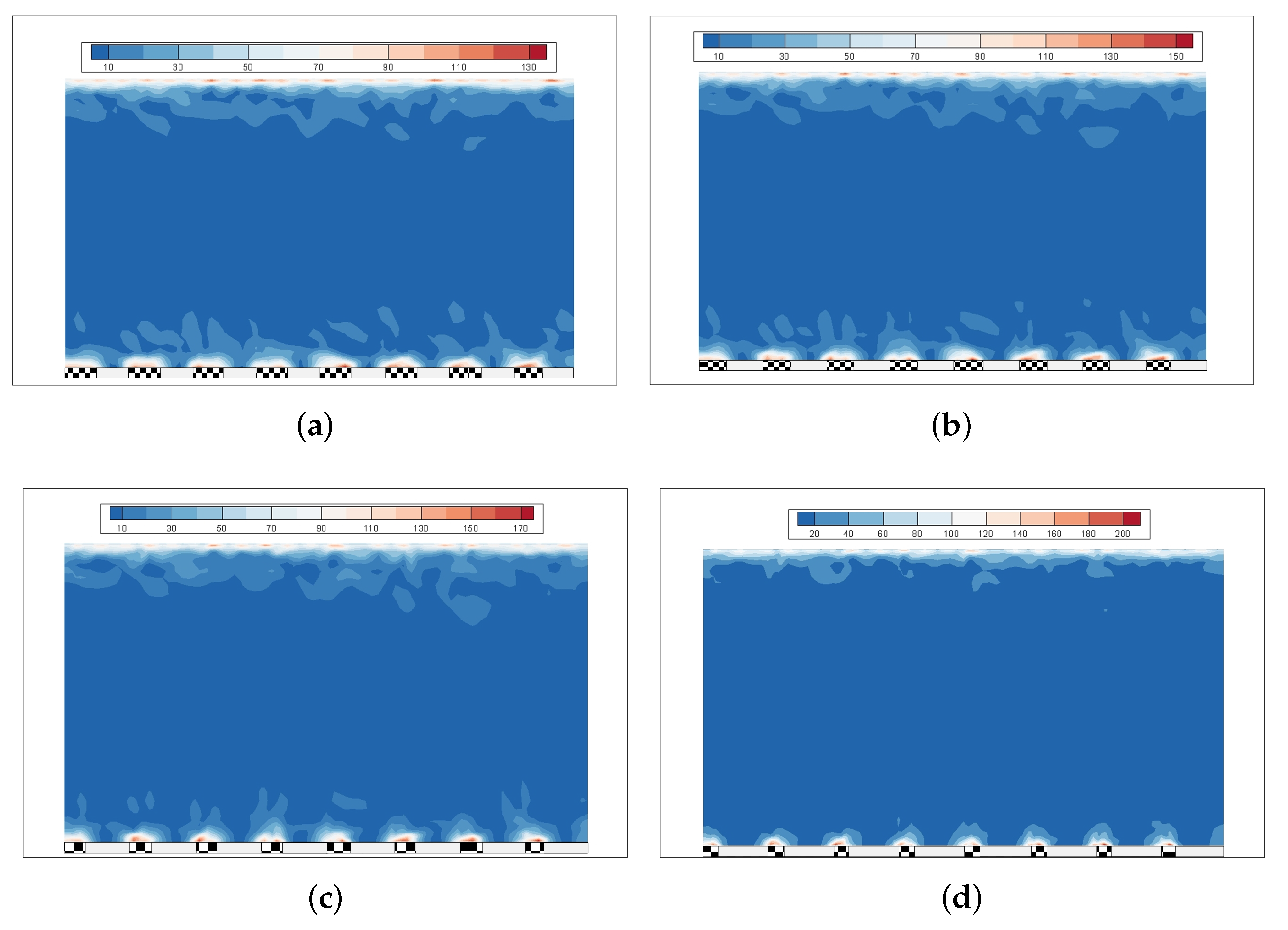
In consideration of the interactive influence of alternating boundary, we studied the vorticity of at different GF. As the Figure 12 shown, the interactive influences of free-slip and no-slip boundary decrease when GF increases.
For the turbulent structure changes on superhydrophobic surfaces, we have concluded that the boundary with strips of small number, such as , can develop a relatively stable flow. For the surface with strips of large number, such as , the alternation of free-slip and no-slip boundary strongly influences the near-wall properties. The continuous shear stress changes on the alternating boundary causes the velocity difference of adjacent fluids to generate more transverse vortices and influences the noise reduction effect. Therefore, the vorticity level near the surfaces of is higher compared with . However, the vorticity in the stable area at the center of the flow field is still reduced compared with the no-slip channel. As a result, the noise reduction effect is weakened when the number of strips increases in a spanwise period.
3.2. Noise Reduction Effect of Strip Numbers
Under the same GF, namely free-slip boundary fraction on superhydrophobic surfaces, different numbers of microstructures in a spanwise period can generate different slip velocities and further influences the noise reduction effect. In this study, the velocity is united by the friction velocity , , and other second-order variables are united by . Then, our results are compared with the logarithmic law. The obtained velocity distribution near the wall has a certain deviation due to the accuracy of LES, and the parameters in the logarithmic law need to be changed.
In this equation, is Karmen constant and C in our study is 0.65. After time average in a flow time period and space average in the streamwise and spanwise direction, the following calculation results are obtained, as shown in Figure 13. The near-wall velocity profile corresponds to the logarithmic law. At the range of , the linear law of is satisfied; at the range of , the logarithmic law of is satisfied.
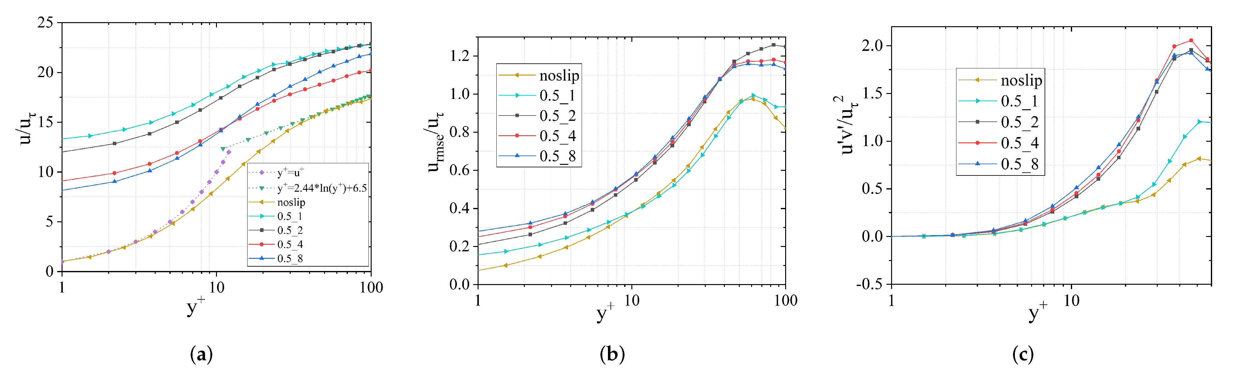
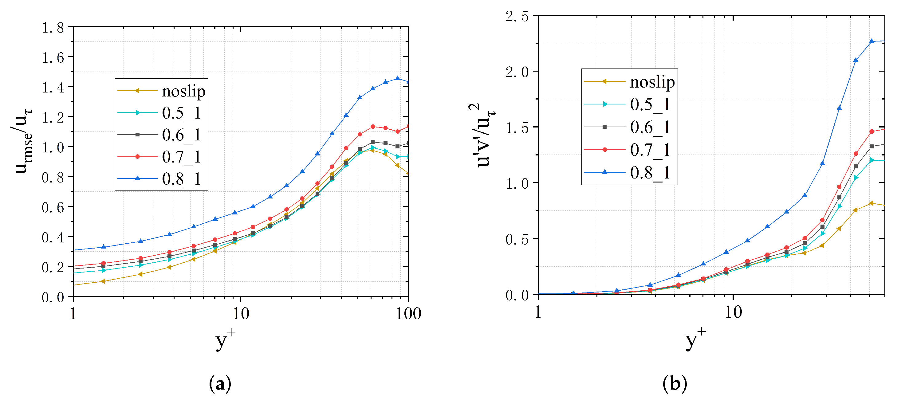
Under the same , we calculated scenarios of different numbers n of free-slip strips in a spanwise period. Notably, . Figure 13 and Figure 14 are the near-wall velocity profiles on superhydrophobic surfaces at and no-slip wall, respectively. The slip velocity can be observed on superhydrophobic surfaces at . Furthermore, it decreases with the increase in the number of free-slip stripes. Figure 13b indicates that the root mean square error (RMSE) of velocity on superhydrophobic surface has contact with the number of free-slip stripes. The RMSE of the near-wall velocity is greater and the fluctuation of the fluid is stronger when more free-slip strips are generated in a period. This condition results in a larger Reynolds stress value in the logarithmic region. Figure 13c shows that the Reynolds stress increases significantly at when . However, when the , the Reynolds stress increases significantly at . These changes show that the enhancement in velocity fluctuation is affected by Reynolds stress. As the strip number increases, the influence range of Reynolds stress increases. At the same time, the thickness of viscous sublayer reduces, and the range of log law region increases. As a result, the near-wall velocity profiles are shown in Figure 13a. Similarly, velocity distribution on the top wall has same changes.
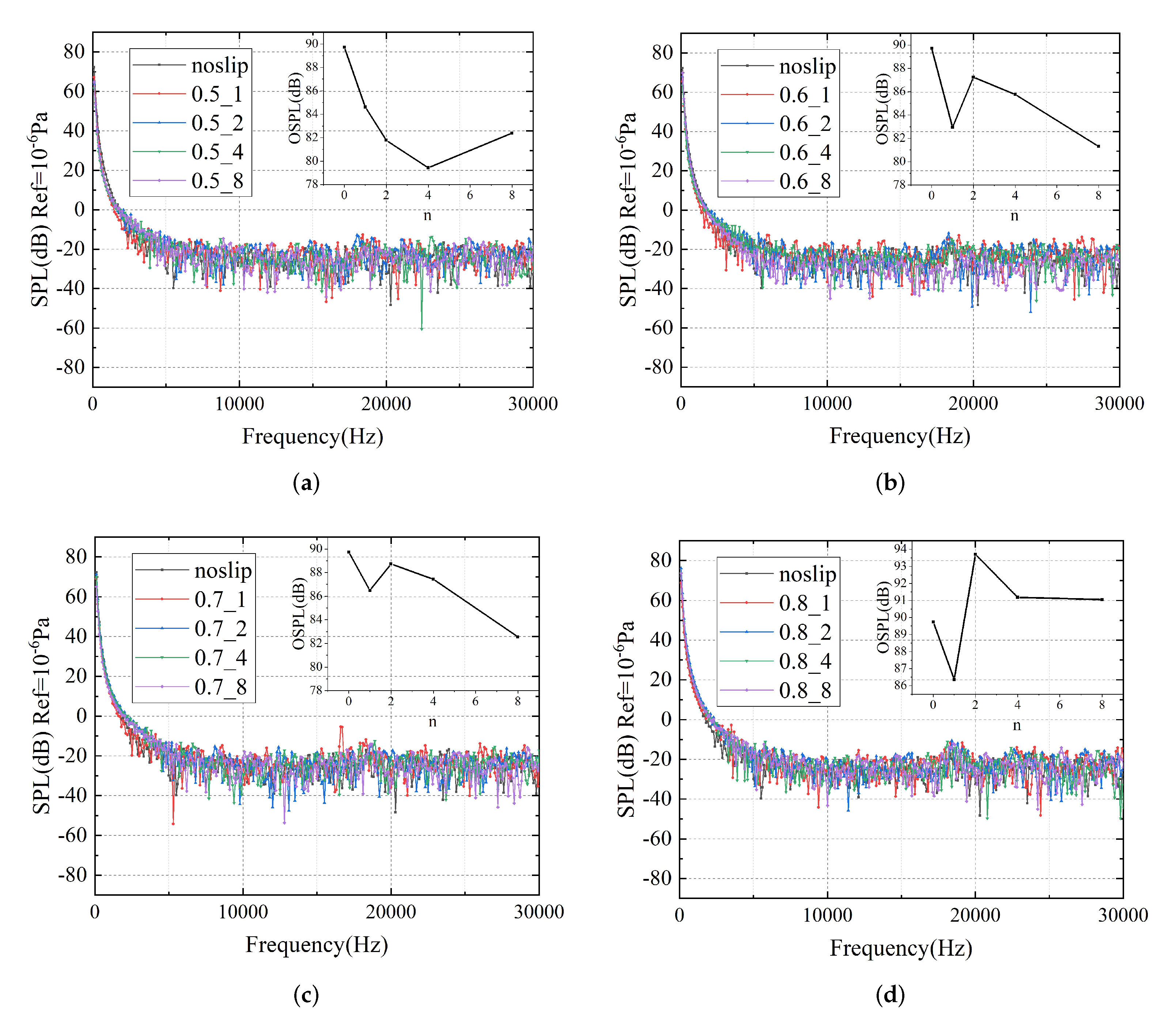
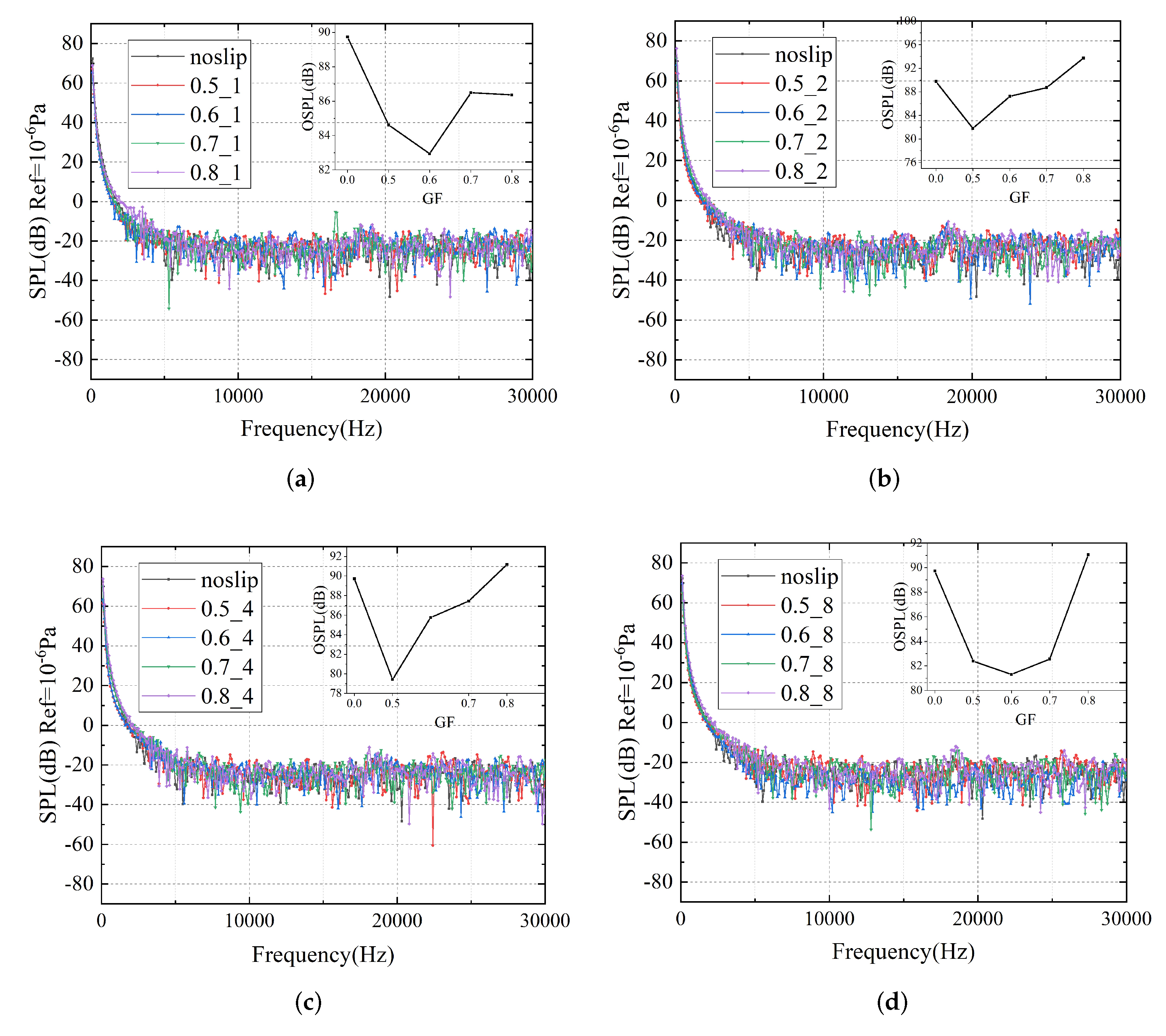
We calculate the flow noise of channel flow at CPG condition and the noise level comparation of different strip numbers at the same GF is shown in Figure 15. The embedded graph in the upper right corner of Figure 15 shows the curve of overall sound pressure level in different scenarios.
When , the overall sound pressure level(OSPL) has a significant reduction compared with that in the no-slip channel at different strip numbers n. The reason is that the free-slip boundary cannot produce a viscous sublayer, the near-wall flow does not have a velocity gradient. Therefore, the energy exchange decreases at different fluid layers and the flow is more stable. As a result, the noise level has a significant reduction.
When , the strip numbers have apparent noise reduction effect. When and , a certain noise reduction effect is exerted, but the effect is poor when . The reason is that the noise increases because the vortex is generated mainly at low frequencies when . Thus, the noise reduction effect is decreased. However, with the increase in slip velocity, the effect of the turbulence and Reynolds stress caused by the increase in the bulk velocity in the channel exceeds the noise reduction effect of superhydrophobic surface. Thus, the noise level can be reduced only at and .
3.3. Noise Reduction Effect of Free-Slip Fraction
This section mainly studies the influence of GF on the drag and the noise reduction effect of superhydrophobic surfaces. The simulation of the free-slip surface with different proportions is realized by controlling the wall shear stress at the bottom of the channel in a period.
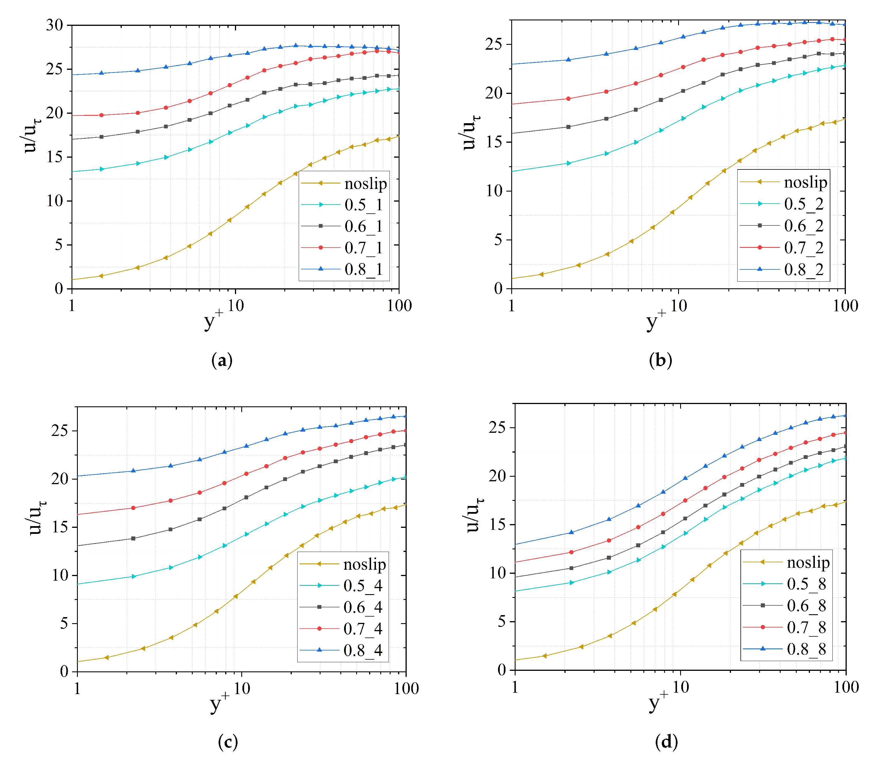
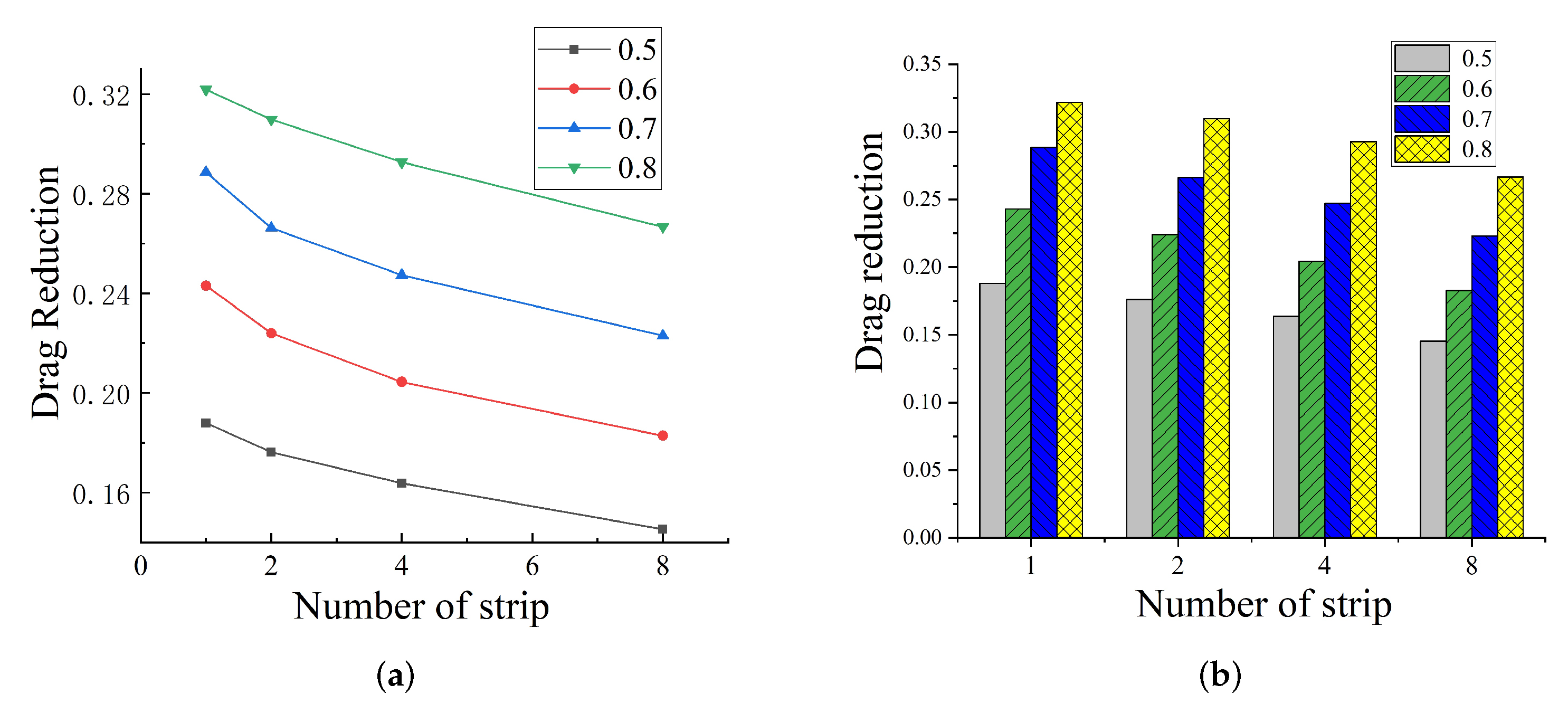
Figure 16 shows the velocity distribution near the wall at different with same numbers of spanwise strips. The results show that slip velocity is greater when the strip number is smaller, and the GF is larger. Under CPG conditions, we define the drag reduction rate as Equation (11)
where is the average velocity of ordinary no-slip channel, and is the average velocity of superhydrophobic channels with different parameters. The results are shown in Figure 17.
At , DR reaches a maximum value of 32%. When the strip number in a spanwise period is 8, the drag reduction effect is approximately 16%, as shown in Figure 17. When n is 1, the velocity RMSE and Reynolds stress of different GF are shown in Figure 18. As the velocity RMSE and the Reynolds stress increase, the linear sublayer becomes thinner. Otherwise, the increase in strip number near the wall accelerates the exchange of fluid momentum and forms more small vortices, therefore the shear stress between the wall and the fluid are increased. Then, the drag reduction effect is decreased.
Figure 19 is the noise level under different GF when the number of strips is fixed. As shown in Figure 19a, the superhydrophobic surfaces with different GF have a certain noise reduction effect. Under the same strip number n, the noise reduction effect increases firstly as the GF increases and then decreases. When , the increase of the overall flow velocity in the channel increases the overall noise level and makes the noise reduction effect of superhydrophobicity no longer obvious. In summary, both GF and strip number should have a suitable range. If the strip number is too small, the gas layer must be unstable. If the GF is too large, the noise level increases. Therefore, comprehensive consideration should be given to noise reduction and drag reduction effect when the superhydrophobic surface is used. The overall sound pressure level is exhibited in Table 4. When strips number is 4 and the GF is 0.5, the best noise reduction effect are obtained as 10.7 dB.
4. Conclusions
In this work, we studied the drag and flow noise reduction effects of the superhydrophobic surfaces with different GF and strip numbers under the same Reynolds number. We used the boundary conditions of alternating free-slip and no-slip surfaces to simulate the superhydrophobic surfaces. The study focuses on the scenario that the Reynolds number is 4200 and the friction Reynolds number is 180. and are considered on the superhydrophobic surfaces to study noise and drag reduction effect. We have used the large eddy simulation for the simulation of the flow domain. We used the Lighthill acoustic analogy combined with finite element and infinite element method for the calculation of the flow noise. The results show that the superhydrophobic surface has noise reduction effect. GF and strip number have a significant influence on the noise reduction effect of the superhydrophobic surface. When GF is small(), superhydrophobic surface will produce a small slip velocity. As a result, the flow is relatively stable and quiet. When GF becomes larger, the bulk velocity in the channel rises and the noise increases due to the increase of slip velocity. When the GF is constant, if n is increased, the fluid in the channel will increase the lateral energy exchange due to the alternating free-slip and no-slip boundary conditions. As a result, more lateral vortex structures are generated and the effect of drag reduction and noise reduction is weakened. In our results, when strip number is 4 and GF is 0.5, the optimal noise reduction effect is obtained as 10.7 dB. The optimal drag reduction effect is 32%, and it is obtained under the scenario of and . In summary, the choice of GF and the number of strips is comprehensively considered to guarantee the performance of drag reduction and noise reduction in this work. This work can provide a new direction for flow noise control on sonar platform.
Author Contributions
Methodology, C.N., Y.L., D.S, C.Z.; software; C.N.; writing—original draft preparation, C.N.; writing—review and editing, C.N., Y.L., D.S., C.Z.; supervision, D.S. All authors have read and agreed to the published version of the manuscript.
Funding
This research was funded by National Defense Basic Scientific Research Program of China, grant number JCKYS2020604SSJS001.
Acknowledgments
The authors would like to thank the College of Underwater Acoustic Engineering Laboratory.
Conflicts of Interest
The authors declare no conflict of interest.
References
- Kim, S.; Kinnas, S.A. Prediction of Unsteady Developed Tip Vortex Cavitation and Its Effect on the Induced Hull Pressures. J. Mar. Sci. Eng. 2020, 8, 114. [Google Scholar] [CrossRef] [Green Version]
- Gloerfelt, X.; Perot, F.; Bailly, C.; Juve, D. Flow-induced cylinder noise formulated as a diffraction problem for low Mach numbers. J. Sound Vib. 2005, 287, 129–151. [Google Scholar] [CrossRef]
- Han, T.; Wang, L.; Cen, K.; Song, B.; Shen, R.Q.; Liu, H.B.; Wang, Q.S. Flow-induced noise analysis for natural gas manifolds using LES and FW-H hybrid method. Appl. Acoust. 2020, 159, 107101. [Google Scholar] [CrossRef]
- Lu, Z.B.; Halim, D.; Cheng, L. Flow-induced noise control behind bluff bodies with various leading edges using the surface perturbation technique. J. Sound Vib. 2016, 369, 1–15. [Google Scholar] [CrossRef]
- Rui, D.; Zezhen, Z.; Fuzhen, P.; Tiecheng, W.; Wanzhen, L. Investigating the sound power level of a simplified underwater vehicle induced by flow separation. Ocean. Eng. 2020, 204, 107286. [Google Scholar] [CrossRef]
- Barbarino, M.; Ilsami, M.; Tuccillo, R.; Federico, L. Combined CFD-Stochastic Analysis of an Active Fluidic Injection System for Jet Noise Reduction. Appl. Sci. 2017, 7, 623. [Google Scholar] [CrossRef] [Green Version]
- Kim, K.S.; Ku, G.r.; Lee, S.J.; Park, S.G.; Cheong, C. Wavenumber-Frequency Analysis of Internal Aerodynamic Noise in Constriction-Expansion Pipe. Appl. Sci. 2017, 7, 1137. [Google Scholar] [CrossRef] [Green Version]
- Al-Okbi, Y.; Chong, T.P.; Stalnov, O. Leading Edge Blowing to Mimic and Enhance the Serration Effects for Aerofoil. Appl. Sci. 2021, 11, 2593. [Google Scholar] [CrossRef]
- Dang, Z.; Mao, Z.; Tian, W. Reduction of Hydrodynamic Noise of 3D Hydrofoil with Spanwise Microgrooved Surfaces Inspired by Sharkskin. J. Mar. Sci. Eng. 2019, 7, 136. [Google Scholar] [CrossRef] [Green Version]
- Liu, Y.; Li, Y.; Shang, D. The Hydrodynamic Noise Suppression of a Scaled Submarine Model by Leading-Edge Serrations. J. Mar. Sci. Eng. 2019, 7, 68. [Google Scholar] [CrossRef] [Green Version]
- Chandrika, U.K.; Pallayil, V.; Lim, K.M.; Chew, C.H. Flow noise response of a diaphragm based fibre laser hydrophone array. Ocean. Eng. 2014, 91, 235–242. [Google Scholar] [CrossRef]
- Corcos, G. Resolution of pressure in turbulence. J. Acoust. Soc. Am. 1963, 35, 192–199. [Google Scholar] [CrossRef]
- Jordan, S.A. A simple model of axisymmetric turbulent boundary layers along long thin circular cylinders. Phys. Fluids 2014, 26, 085110. [Google Scholar] [CrossRef]
- Karthik, K.; Vengadesan, S.; Bhattacharyya, S.K. Prediction of flow induced sound generated by cross flow past finite length circular cylinders. J. Acoust. Soc. Am. 2018, 143, 260. [Google Scholar] [CrossRef]
- Pallayil, V.; Chotiros, N.P. AUV-Based Seabed Characterisation Using a Lightweight Towed Array System. In Proceedings of the Offshore Technology Conference Asia, Houston, TX, USA, 2–5 May 2016. [Google Scholar]
- Willmarth, W.; Yang, C. Wall-pressure fluctuations beneath turbulent boundary layers on a flat plate and a cylinder. J. Fluid Mech. 1970, 41, 47–80. [Google Scholar] [CrossRef]
- Cassie, A.B.D.; Baxter, S. Wettability of porous surfaces. Trans. Faraday Soc. 1944, 40, 546–551. [Google Scholar] [CrossRef]
- Philip, J.R. Flows satisfying mixed no-slip and no-shear conditions. Z. Für Angew. Math. Und Phys. ZAMP 1972, 23, 353–372. [Google Scholar] [CrossRef]
- Choi, C.H.; Westin, K.J.A.; Breuer, K.S. Apparent slip flows in hydrophilic and hydrophobic microchannels. Phys. Fluids 2003, 15, 2897–2902. [Google Scholar] [CrossRef]
- Ou, J.; Perot, B.; Rothstein, J.P. Laminar drag reduction in microchannels using ultrahydrophobic surfaces. Phys. Fluids 2004, 16, 4635–4643. [Google Scholar] [CrossRef] [Green Version]
- Joseph, P.; Tabeling, P. Direct measurement of the apparent slip length. Phys. Rev. E Stat. Nonlin. Soft Matter Phys. 2005, 71, 035303. [Google Scholar] [CrossRef]
- Park, H.; Park, H.; Kim, J. A numerical study of the effects of superhydrophobic surface on skin-friction drag in turbulent channel flow. Phys. Fluids 2013, 25, 66001. [Google Scholar] [CrossRef] [Green Version]
- Truesdell, R.; Mammoli, A.; Vorobieff, P.; van Swol, F.; Brinker, C.J. Drag reduction on a patterned superhydrophobic surface. Phys. Rev. Lett. 2006, 97, 044504. [Google Scholar] [CrossRef]
- Min, T.G.; Kim, J. Effects of hydrophobic surface on skin-friction drag. Phys. Fluids 2004, 16, L55–L58. [Google Scholar] [CrossRef]
- Martell, M.B.; Perot, J.B.; Rothstein, J.P. Direct numerical simulations of turbulent flows over superhydrophobic surfaces. J. Fluid Mech. 2009, 620, 31–41. [Google Scholar] [CrossRef] [Green Version]
- Martell, M.B.; Rothstein, J.P.; Perot, J.B. An analysis of superhydrophobic turbulent drag reduction mechanisms using direct numerical simulation. Phys. Fluids 2010, 22, 065102. [Google Scholar] [CrossRef] [Green Version]
- Jalalabadi, R.; Hwang, J.; Nadeem, M.; Yoon, M.; Sung, H.J. Turbulent boundary layer over a divergent convergent superhydrophobic surface. Phys. Fluids 2017, 29, 085112. [Google Scholar] [CrossRef]
- Turk, S.; Daschiel, G.; Stroh, A.; Hasegawa, Y.; Frohnapfel, B. Turbulent flow over superhydrophobic surfaces with streamwise grooves. J. Fluid Mech. 2014, 747, 186–217. [Google Scholar] [CrossRef]
- Seo, J.; García-Mayoral, R.; Mani, A. Pressure fluctuations and interfacial robustness in turbulent flows over superhydrophobic surfaces. J. Fluid Mech. 2015, 783, 448–473. [Google Scholar] [CrossRef] [Green Version]
- Fairhall, C.T.; Abderrahaman-Elena, N.; Garcia-Mayoral, R. The effect of slip and surface texture on turbulence over superhydrophobic surfaces. J. Fluid Mech. 2019, 861, 88–118. [Google Scholar] [CrossRef] [Green Version]
- Rastegari, A.; Akhavan, R. The common mechanism of turbulent skin-friction drag reduction with superhydrophobic longitudinal microgrooves and riblets. J. Fluid Mech. 2018, 838, 68–104. [Google Scholar] [CrossRef]
- Rastegari, A.; Akhavan, R. On drag reduction scaling and sustainability bounds of superhydrophobic surfaces in high Reynolds number turbulent flows. J. Fluid Mech. 2019, 864, 327–347. [Google Scholar] [CrossRef]
- Im, H.J.; Lee, J.H. Comparison of superhydrophobic drag reduction between turbulent pipe and channel flows. Phys. Fluids 2017, 29, 095101. [Google Scholar] [CrossRef]
- Costantini, R.; Mollicone, J.P.; Battista, F. Drag reduction induced by superhydrophobic surfaces in turbulent pipe flow. Phys. Fluids 2018, 30, 025102. [Google Scholar] [CrossRef]
- Daniello, R.J.; Waterhouse, N.E.; Rothstein, J.P. Drag reduction in turbulent flows over superhydrophobic surfaces. Phys. Fluids 2009, 21, 085103. [Google Scholar] [CrossRef] [Green Version]
- Fukagata, K.; Kasagi, N.; Koumoutsakos, P. A theoretical prediction of friction drag reduction in turbulent flow by superhydrophobic surfaces. Phys. Fluids 2006, 18, 051703. [Google Scholar] [CrossRef]
- Zhang, J.X.; Tian, H.P.; Yao, Z.H.; Hao, P.F.; Jiang, N. Mechanisms of drag reduction of superhydrophobic surfaces in a turbulent boundary layer flow. Exp. Fluids 2015, 56, 179. [Google Scholar] [CrossRef]
- Abu Rowin, W.; Ghaemi, S. Streamwise and spanwise slip over a superhydrophobic surface. J. Fluid Mech. 2019, 870, 1127–1157. [Google Scholar] [CrossRef]
- Gose, J.W.; Golovin, K.; Boban, M.; Mabry, J.M.; Tuteja, A.; Perlin, M.; Ceccio, S.L. Characterization of superhydrophobic surfaces for drag reduction in turbulent flow. J. Fluid Mech. 2018, 845, 560–580. [Google Scholar] [CrossRef] [Green Version]
- Aljallis, E.; Sarshar, M.A.; Datla, R.; Sikka, V.; Jones, A.; Choi, C.H. Experimental study of skin friction drag reduction on superhydrophobic flat plates in high Reynolds number boundary layer flow. Phys. Fluids 2013, 25, 025103. [Google Scholar] [CrossRef]
- Ybert, C.; Barentin, C.; Cottin-Bizonne, C.; Joseph, P.; Bocquet, L. Achieving large slip with superhydrophobic surfaces: Scaling laws for generic geometries. Phys. Fluids 2007, 19, 123601. [Google Scholar] [CrossRef]
- Lighthill, M.J. On sound generated aerodynamically. Philos. Trans. R. Soc. A 1952, 211, 564–587. [Google Scholar]
- Bossart, R.; Joly, N.; Bruneau, M. Hybrid numerical and analytical solutions for acoustic boundary problems in thermo-viscous fluids. J. Sound Vib. 2003, 263, 69–84. [Google Scholar] [CrossRef]
- Lafon, P.; Caillaud, S.; Devos, J.P.; Lambert, C. Aeroacoustical coupling in a ducted shallow cavity and fluid/structure effects on a steam line. J. Fluids Struct. 2003, 18, 695–713. [Google Scholar] [CrossRef]
Figure 1.
Schematic of streamwise strip on superhydrophobic surface. (a) Alternating free-slip and no-slip boundary condition. (b) Diagram of slip velocity.
Figure 1.
Schematic of streamwise strip on superhydrophobic surface. (a) Alternating free-slip and no-slip boundary condition. (b) Diagram of slip velocity.

Figure 2.
Diagram of flow domain size and boundary condition.

Figure 3.
Mean streamwise velocity normalized with . The dashed yellow line is the theoretical prediction in the viscous sublayer. The dashed blue line is the fit in log-layer region.
Figure 3.
Mean streamwise velocity normalized with . The dashed yellow line is the theoretical prediction in the viscous sublayer. The dashed blue line is the fit in log-layer region.

Figure 4.
Diagram of Lafon’ experiment.

Figure 5.
Comparison of the simulation results and Lafon’ experiment data. The black line is simulation results. The red line is Lafon’ experiment data.
Figure 5.
Comparison of the simulation results and Lafon’ experiment data. The black line is simulation results. The red line is Lafon’ experiment data.

Figure 6.
Schematic of sound simulation domain.

Figure 7.
Boundary condition of sound simulation domain and hydrophone array.

Figure 8.
Contours of pressure distribution at the bottom wall of channel. (a) no-slip. (b) . (c) . (d) . (e) .
Figure 8.
Contours of pressure distribution at the bottom wall of channel. (a) no-slip. (b) . (c) . (d) . (e) .

Figure 9.
Comparison of pressure RMSE at the bottom wall of channel(superhydrophobic surface). (a) , . (b) , .
Figure 9.
Comparison of pressure RMSE at the bottom wall of channel(superhydrophobic surface). (a) , . (b) , .

Figure 10.
cutplane contours of vorticity at different strip numbers.

Figure 11.
Streamlines at the cutplane. (a) no-slip. (b) . (c) . (d) . (e) .

Figure 12.
Comparison of vorticity for different GF at . (a) . (b) . (c) (d) .

Figure 13.
Comparison of statistics for and at the bottom wall of channel (superhydrophobic surface). (a) Mean streamwise velocity profile. (b) Velocity RMSE fluctuations. (c) Reynolds stress.
Figure 13.
Comparison of statistics for and at the bottom wall of channel (superhydrophobic surface). (a) Mean streamwise velocity profile. (b) Velocity RMSE fluctuations. (c) Reynolds stress.

Figure 14.
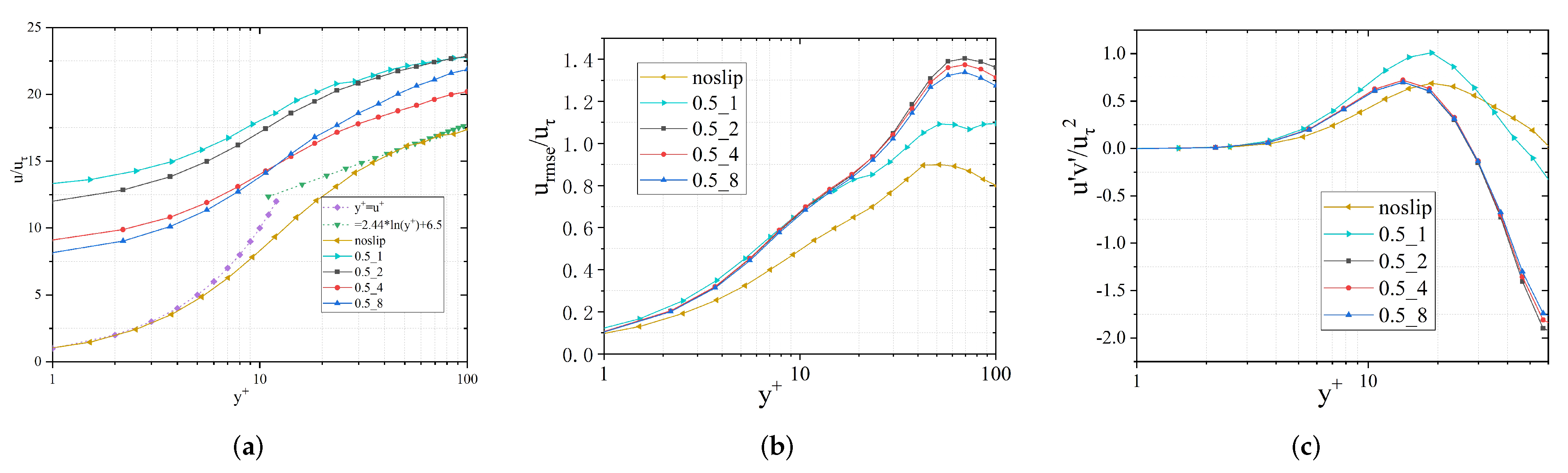
Comparison of statistics for and at the top wall of the channel (no-slip surface). (a) Mean streamwise velocity profile. (b) Velocity RMSE fluctuations. (c) Reynolds stress.
Figure 14.
Comparison of statistics for and at the top wall of the channel (no-slip surface). (a) Mean streamwise velocity profile. (b) Velocity RMSE fluctuations. (c) Reynolds stress.

Figure 15.
Comparison of frequency spectra for different strips number at . (a) . (b) . (c) (d) .

Figure 16.
Comparison of mean velocity for same strips number at different GF. (a) , . (b) , . (c) , . (d) , .
Figure 16.
Comparison of mean velocity for same strips number at different GF. (a) , . (b) , . (c) , . (d) , .

Figure 17.
Drag reduction effect of superhydrophobic surfaces at different scenarios. (. ).

Figure 18.
Caparison of statistics for at different GF. (a) Velocity RMSE. (b) Reynolds number.

Figure 19.
Comparison of frequency spectra for GF at . (a) . (b) . (c) (d) .


Table 1.
Simulation parameters. Gas fraction is the area ratio of free-slip to no-slip surface. Strip number represent the number of strips in a spanwise period. is friction Reynolds number. Grid number is the number of point for streamwise, wall-normal, and spanwise directions.
Table 1.
Simulation parameters. Gas fraction is the area ratio of free-slip to no-slip surface. Strip number represent the number of strips in a spanwise period. is friction Reynolds number. Grid number is the number of point for streamwise, wall-normal, and spanwise directions.
| Domain Size | Gas Fraction | Strip Number | Grid Number () | ||||
|---|---|---|---|---|---|---|---|
| GF = 0.5 | 1, 2, 4, 8 | 150 × 60 × 80 | 180 | 3 | 0.3 | 3 | |
| GF = 0.6 | 1, 2, 4, 8 | 150 × 60 × 80 | 180 | 3 | 0.3 | 3 | |
| GF = 0.7 | 1, 2, 4, 8 | 150 × 60 × 96 | 180 | 3 | 0.3 | 3 | |
| GF = 0.8 | 1, 2, 4, 8 | 150 × 60 × 112 | 180 | 3 | 0.3 | 3 |
Table 2.
Grid and Wale constant independence validation. is drag coefficient on the bottom wall, is Smagorinsky constant, is Wale constant.
Table 2.
Grid and Wale constant independence validation. is drag coefficient on the bottom wall, is Smagorinsky constant, is Wale constant.
| Mesh Size | Mesh Size | ||||
|---|---|---|---|---|---|
| 130 × 40 × 60 | 0.001307 | 150 × 60 × 80 | 0.1 | 0.32 | 0.001294 |
| 140 × 50 × 70 | 0.001291 | ||||
| 150 × 60 × 80 | 0.001294 | 0.18 | 0.55 | 0.001288 | |
| 160 × 70 × 90 | 0.001288 |
Table 3.
Model parameter of Lafon’ experiment.
| = 61.2 m/s | h = 0.02 m | H = 0.137 m |
| d = 0.05 m | L = 0.073 m |
Table 4.
Overall sound pressure level of different scenarios (dB).
| Strips Number | 1 | 2 | 4 | 8 |
|---|---|---|---|---|
| GF = 0.5 | 84.6 | 81.5 | 79.2 | 82.6 |
| GF = 0.6 | 83.1 | 87.1 | 85.9 | 81.2 |
| GF = 0.7 | 86.5 | 88.6 | 87.5 | 82.5 |
| GF = 0.8 | 86.2 | 93.5 | 91.1 | 90.8 |
| no-slip | 89.9 dB | |||
Publisher’s Note: MDPI stays neutral with regard to jurisdictional claims in published maps and institutional affiliations. |
© 2021 by the authors. Licensee MDPI, Basel, Switzerland. This article is an open access article distributed under the terms and conditions of the Creative Commons Attribution (CC BY) license (https://creativecommons.org/licenses/by/4.0/).
Share and Cite
MDPI and ACS Style
Niu, C.; Liu, Y.; Shang, D.; Zhang, C. Noise Reduction Effect of Superhydrophobic Surfaces with Streamwise Strip of Channel Flow. Appl. Sci. 2021, 11, 3869. https://0-doi-org.brum.beds.ac.uk/10.3390/app11093869
AMA Style
Niu C, Liu Y, Shang D, Zhang C. Noise Reduction Effect of Superhydrophobic Surfaces with Streamwise Strip of Channel Flow. Applied Sciences. 2021; 11(9):3869. https://0-doi-org.brum.beds.ac.uk/10.3390/app11093869
Chicago/Turabian StyleNiu, Chen, Yongwei Liu, Dejiang Shang, and Chao Zhang. 2021. "Noise Reduction Effect of Superhydrophobic Surfaces with Streamwise Strip of Channel Flow" Applied Sciences 11, no. 9: 3869. https://0-doi-org.brum.beds.ac.uk/10.3390/app11093869
Note that from the first issue of 2016, this journal uses article numbers instead of page numbers. See further details here.