A Survey of Low-Cost 3D Laser Scanning Technology

1
Robotics Institute, Beihang University, Beijing 100191, China
2
Institute of Informatization and Industrialization Integration, China Academy of Information and Communications Technology (CAICT), Beijing 100191, China
*
Author to whom correspondence should be addressed.
Appl. Sci. 2021, 11(9), 3938; https://0-doi-org.brum.beds.ac.uk/10.3390/app11093938
Submission received: 15 March 2021
/
Revised: 17 April 2021
/
Accepted: 25 April 2021
/
Published: 27 April 2021
(This article belongs to the Special Issue Laser Sensing in Robotics)
Abstract
:By moving a commercial 2D LiDAR, 3D maps of the environment can be built, based on the data of a 2D LiDAR and its movements. Compared to a commercial 3D LiDAR, a moving 2D LiDAR is more economical. A series of problems need to be solved in order for a moving 2D LiDAR to perform better, among them, improving accuracy and real-time performance. In order to solve these problems, estimating the movements of a 2D LiDAR, and identifying and removing moving objects in the environment, are issues that should be studied. More specifically, calibrating the installation error between the 2D LiDAR and the moving unit, the movement estimation of the moving unit, and identifying moving objects at low scanning frequencies, are involved. As actual applications are mostly dynamic, and in these applications, a moving 2D LiDAR moves between multiple moving objects, we believe that, for a moving 2D LiDAR, how to accurately construct 3D maps in dynamic environments will be an important future research topic. Moreover, how to deal with moving objects in a dynamic environment via a moving 2D LiDAR has not been solved by previous research.
1. Introduction
Three-dimensional (3D) laser scanning technology, an advanced surveying and mapping method, has obvious advantages compared to traditional techniques. It combines high efficiency with data quality and accuracy. As the core sensor of 3D laser scanning technology, 3D LiDAR is widely used in many applications, such as terrain survey [1], architectural surveying and mapping [2], automatic driving [3], forest monitoring [4], and plant analysis [5].
However, for the moment, 3D LiDAR is generally expensive and is not consumer-grade yet. In comparison, 2D LiDAR is much more economical, and some 2D LiDARs are already consumer-grade [6]. As two major categories of commercial LiDAR, the differences between 2D LiDAR and 3D LiDAR are as follows: a 2D LiDAR is more economical than a 3D LiDAR, but it obtains less information, and it can only build 2D maps of the environment. On the other hand, a 3D LiDAR can build 3D maps of the environment; however, it is far more expensive than 2D LiDAR. Figure 1 shows a comparison of the maps built by a 2D LiDAR and a 3D LiDAR, respectively. We investigated some commonly used commercial 2D LiDARs and 3D LiDARs; their manufacturers, models, performances, prices, and application fields are listed in Table A1 of Appendix A to provide readers with a more detailed understanding of them.
By moving a commercial 2D LiDAR, 3D maps of the environment can be built based on the data of the 2D LiDAR and its movement [8,9,10,11]. Compared with a commercial 3D LiDAR, a moving 2D LiDAR is more economical, while its measurement performance is far inferior to that of the former. For applications that do not require excess measurement performance and require strict cost control (such as the 3D perception of the environment by a commercial home service robot), a moving 2D LiDAR may be useful. From this perspective, a moving 2D LiDAR is necessary and research-worthy.
It must be emphasized that a moving 2D LiDAR cannot completely replace a 3D LiDAR. In some applications, with high requirements on real-time performance and measurement ranges, such as automatic driving, a 3D LiDAR with better real-time performance and a longer measurement range is required, while a moving 2D LiDAR is not adequate. However, in other applications, such as the 3D mapping and navigation of an indoor robot, a moving 2D LiDAR can do the job. In these applications, a moving 2D LiDAR can partially replace a 3D LiDAR and provide a new choice for developers and engineers, which can reduce the costs, while the basic functions of 3D mapping are ensured.
In addition, a moving 2D LiDAR has the advantages of a flexible field of view and angular resolution. The field of view and angular resolution of a moving 2D LiDAR depend on the movement of the 2D LiDAR. Customizing scan parameters by moving LiDAR is not unique to 2D LiDAR. In [11,12,13,14,15,16,17,18,19], since the field of view and angular resolution of some 3D LiDARs are not suitable, researchers obtained the field of view and angular resolutions they wanted by moving these LiDARs.
Although low-cost 3D laser scanning technology based on a moving 2D LiDAR is needed in some applications, as far as we know, survey in this research field is relatively unexplored. In view of this, in this paper, we present our survey of low-cost 3D laser scanning technology.
At present, there are problems in the application of a moving 2D LiDAR. First, there is the problem of accuracy, primarily due to the error of the 2D LiDAR movement estimation. Specifically, this error may originate from the installation error between the 2D LiDAR and the moving unit [10,20,21,22,23,24,25,26,27,28,29,30,31,32,33,34,35], or it may originate from the inaccurate movement estimation of the moving unit [36,37,38,39,40,41].
Second, the real-time performance of a moving 2D LiDAR is poor (generally, its 3D scanning frequency is lower than 1 Hz), which makes it difficult to be utilized in applications that require real-time performance. Therefore, when there are moving objects in the environment, a moving 2D LiDAR is not likely to capture their shapes. Therefore, for a moving 2D LiDAR, the recognition and removal of moving objects is a problem that needs to be solved [42,43]. For a commercialized 3D LiDAR, the process of moving objects is simple and mature [44,45,46,47], but for a moving 2D LiDAR, the process of moving objects is much more difficult and relatively unexplored, because the shape of a moving object is difficult to be accurately captured by a moving 2D LiDAR.
In addition to the above two core issues, namely accuracy and real-time performance, for a moving 2D LiDAR, there are some other research topics. For example, the density distribution of the 3D point cloud collected by a moving 2D LiDAR [48,49,50,51,52,53], the fusion of a moving 2D LiDAR and 2D SLAM [54,55,56,57], the detection of obstacles in front of the vehicle or road edge by a push-broom 2D LiDAR [58,59,60,61], and the fusion of a moving 2D LiDAR and camera [62,63,64,65,66,67], etc.
Moreover, due to the diversity of prototypes (in essence, it is the diversity of the ways to move 2D LiDARs) [16,20,36,37,38,48,50,51,52,53,68,69,70,71,72,73,74,75,76,77,78,79,80,81], for each category of prototype, the specific sub-topics corresponding to the above research topics may be different. In our paper, these sub-topics are classified and discussed.
The rest of this paper is structured as follows: Section 2 describes the overview of the principle of a moving 2D LiDAR. We classify a moving 2D LiDAR by the movement of the 2D LiDAR in Section 3. In Section 4, we present the problems that need to be solved in the application of a moving 2D LiDAR. In Section 5, we clarify a few issues. Finally, we present the conclusions in Section 6.
The notations used throughout this paper are listed in Table A2, which is in Appendix B.
2. Overview of Principles
We begin the discussion of a moving 2D LiDAR by analyzing its principles. Here, the widely used TOF (Time of Flight) LiDAR is taken as an example. When a TOF LiDAR is working, the emitter in it emits laser beams. The laser beams are reflected after encountering objects and are received by the receiver of the LiDAR. The TOF LiDAR calculates the distance of an observed object by the time difference between the point in time when a laser beam is emitted, and the point in time when a laser beam returns after reflection.
In Figure 2, a TOF 2D LiDAR collects two sets of data at positions 1 and 2 in a room, respectively. At each position, in the fan-shaped scanning area of the 2D LiDAR, its emitter emits a certain number of laser beams, some of which shoot out of the door or window of the room, and do not reflect back. The remaining light beams encounter the objects or walls in the room, and reflect back. Those laser beams are received by the receiver of the 2D LiDAR, from which sampling points can be calculated.
The principle of a moving 2D LiDAR can be briefly summarized in one sentence, which is, 2D LiDAR collects sampling points at different positions, and these sampling points are converted to a global world coordinate frame. This process involves the conversion of the 3D coordinates of the sampling point between different coordinate frames. Here, we define three coordinate frames, namely, the coordinate frame of the 2D LiDAR (at position 1), which is denoted as L-XLYLZL; the coordinate frame of the 2D LiDAR at another position (position 2), which is denoted as L′-XL′YL′ZL′; the world coordinate frame W-XWYWZW, as shown in Figure 2.
The definition of the 2D LiDAR coordinate frame L-XLYLZL is as follows: the original point L of this coordinate frame is the center of the 2D LiDAR scanning sector. The plane YLLZL is a coplanar with the scanning sector. The axis ZL is the middle line of the scanning sector, and the axis XL is perpendicular to the scanning sector. The position of coordinate frame L relative to the 2D LiDAR is fixed, but its position relative to the room is not fixed, because the 2D LiDAR is moving in the room.
The definition of the coordinate frame L′-XL′YL′ZL′ is similar to the definition of coordinate frame L-XLYLZL. The only difference is that the position of the coordinate frame L′-XL′YL′ZL′ relative to the coordinate frame L-XLYLZL has been changed, for the position of the 2D LiDAR has been changed.
The coordinate frame W-XWYWZW is the global world coordinate frame. Compared with the coordinate frame L-XLYLZL and the coordinate frame L′-XL′YL′ZL′ whose positions are not fixed, the coordinate frame W-XWYWZW is fixed relative to the room. The 3D coordinates of the sampling points collected by the 2D LiDAR at different positions are converted to the coordinate frame W-XWYWZW. In this way, a 3D point cloud that shows the outline of the room can be built.
The raw data collected by a 2D LiDAR contain ranging data and azimuth angles. The ranging data and azimuth angle of point p in Figure 2 are denoted as r and θ, respectively. The coordinate of point p relative to coordinate frame L is denoted as pL, it can be calculated as follows:
where c(·) and s(·) are cos and sin, respectively.
Next, point pL in coordinate frame L is converted to the corresponding point pW in coordinate frame W
where and are the rotation matrix and the translation vector from coordinate frame L to coordinate frame W, respectively.
In this way, the 3D coordinates of the sampling point p relative to the world coordinate frame W can be calculated. For the sampling points of the 2D LiDAR at different positions, methods similar to (1) and (2) can be used to calculate their 3D coordinates, relative to the world coordinate frame W—that is, the first step is to calculate the coordinates of the sampling points relative to the 2D LiDAR coordinate frame, according to the raw data of a 2D LiDAR. The second step is to calculate the coordinates of the sampling points relative to the world coordinate frame by space rigid body transformations.
According to the above principle, in order to ensure the accuracy of the 3D point cloud built by a moving 2D LiDAR, first, the raw data of the 2D LiDAR should be accurate (this depends on the accuracy of the 2D LiDAR), so that the coordinates of the sampling points relative to the 2D LiDAR coordinate frame can be accurately calculated by Equation (1).
Second, the parameters of the space rigid body transformation between the 2D LiDAR coordinate frame and the world coordinate frame need to be accurately known, so that the coordinates of the sampling point relative to the world coordinate frame can be accurately calculated by Equation (2). If the space rigid body transformation parameters are not accurate, the 3D point cloud will be distorted. The research on this issue is important for the improvement of the accuracy of the 3D point cloud built by a moving 2D LiDAR. We will discuss it more in the following sections.
From the above, we can see that there are two factors that determine the accuracy of a moving 2D LiDAR. First, the accuracy of the 2D LiDAR used. Second, the accuracy of the estimation of the movement of the 2D LiDAR.
At present, there is no method to significantly improve the accuracy of 2D LiDAR for researchers—this is the job of the manufacturers. Therefore, to improve the accuracy of a moving 2D LiDAR, we seek to improve the accuracy of the estimation of the movement of 2D LiDAR as much as possible. In the following, some specific topics that need to be studied in order to accurately estimate the movement of 2D LiDAR will be listed and discussed.
We believe that the ideal situation is that the measurement accuracy of a moving 2D LiDAR is consistent with the accuracy of the used 2D LiDAR, because the movement estimation of the 2D LiDAR is accurate enough so that the measurement accuracy of a moving 2D LiDAR will not be affected by it. According to Table A1, the accuracy level of most 2D LiDARs is centimeter-level. In our opinion, for a moving 2D LiDAR (especially for a rotating 2D LiDAR or a pitching 2D LiDAR, for them, the estimation of the movement of the 2D LiDAR is relatively simple and mature), it is feasible to control the systematic error within ±50 mm, which is slightly larger than the systematic errors of most 2D LiDARs in Table A1.
3. Classification of the Prototypes
From a perspective of engineering, a moving 2D LiDAR can be built in many ways. In this section, we classify a moving 2D LiDAR by the most intuitive way, that is, the movement of 2D LiDAR.
For a moving 2D LiDAR, there are three common ways to move the 2D LiDAR, namely rotation, pitching, and push-broom. There is also literature on pitching as nodding [20,38,68]. In our paper, it is collectively referred to as pitching.
In addition to these three categories, there are other categories. We listed our classification in Table 1. Next, we will discuss these categories in detail one-by-one.
3.1. A Rotating 2D LiDAR and a Pitching 2D LiDAR
There are some similarities between a rotating 2D LiDAR and a pitching 2D LiDAR. For both of them, 2D LiDAR is rotated by a motor. The motor changes the attitude of the 2D LiDAR, and, at the same time, another motor inside the 2D LiDAR rotates the emitter, which can emit the laser beam. In this way, the emitter can emit the laser beam into 3D space, and the scanning area of the 2D LiDAR is no longer limited to a 2D plane. There are two rotation axes involved here, one of which is the axis of rotation of the 2D LiDAR, the other is the axis of rotation of the emitter inside the 2D LiDAR.
A rotating 2D LiDAR and a pitching 2D LiDAR are similar in principle. For both of them, the data collected by the 2D LiDAR and the angle position of the motor shaft are combined to calculate the 3D coordinates of the sampling points. According to the general principle of a moving 2D LiDAR analyzed in Section 2, for a rotating 2D LiDAR and a pitching 2D LiDAR, the in Equation (2) is a zero vector, and is the rotation matrix calculated according to the angle position of the motor shaft. The angle position of the motor shaft mentioned here is relative to the initial angle position. The initial angle position of the motor shaft should be recognized as a reference. In order to define the initial angle position of the motor shaft, an absolute encoder or a photoelectric switch is required.
There are some points that need to be noted for both a rotating 2D LiDAR and a pitching 2D LiDAR: the optical center of the 2D LiDAR must coincide with its rotation axis, this depends on the mechanical accuracy; the ranging data of 2D LiDAR must be synchronized with its rotation/pitch angle, the accuracy of synchronization determines the accuracy of the rotation matrix . In addition, the mechanical structure that rotate/pitch the 2D LiDAR should not obstruct the field of view of the 2D LiDAR [69].
The main difference between a rotating 2D LiDAR and a pitching 2D LiDAR is that the rotation axis of a rotating 2D LiDAR coincides with the middle line of the scanning sector, while the rotation axis of a pitching 2D LiDAR is perpendicular to the middle line of the scanning sector and is coplanar with the scanning sector. The rotation angle of a rotating 2D LiDAR should to be no less than 180°, otherwise there will be blind areas in the field of view, while the rotation angle of a pitching 2D LiDAR can be flexibly adjusted according to the need of the field of view, as shown in Figure 3. From this point of view, a pitching 2D LiDAR can scan the front area faster than a rotating 2D LiDAR, and is thus more suitable for the area monitoring of mobile robots [69]. As mentioned in [20], for a rotating 2D LiDAR, when the 2D LiDAR is rotated around an axis parallel to the observation direction, it is suitable for environments such as tunnels or corridors. For a pitching 2D LiDAR, when the 2D LiDAR is rotated around an axis perpendicular to the observation direction, it is suitable for general ground robot applications, because in such applications, dense 3D point clouds that can show the terrain ahead are required.
In actual applications, whether a rotating 2D LiDAR or a pitching 2D LiDAR, the attitude of the rotation axis of the 2D LiDAR is very important. For indoor mobile robots, some of its obstacles are objects with relatively small sizes in the horizontal direction and relatively large sizes in the vertical direction, such as human bodies, pillars, or table legs. In order to avoid the missed detection of these obstacles, the axis of rotation should be horizontal rather than vertical, that is, it should be like (a) and (b) in Figure 4, rather than (c) and (d). In order to increase the scanning speed, the angular resolution of the motor rotation is often lower than the angular resolution of the scanning sector of a 2D LiDAR, so when the rotation axis is horizontal rather than vertical, the missed detection of the above-mentioned obstacles may be more likely to be avoided. Figure 5 shows the prototypes in [20,38,48,68,69].
3.2. A Push-Broom 2D LiDAR
Compared with a rotating 2D LiDAR and a pitching 2D LiDAR, the main feature of a push-broom 2D LiDAR is that there is no relative movement between the 2D LiDAR and the mobile platform on which it is carried, the 2D LiDAR is fixedly assembled on the mobile platform. The mobile platform mentioned here may be a vehicle [36,37,70,71], a backpack [16,72,73], a handheld pole [74,75], or a UAV (unmanned aerial vehicle) [76,77], as shown in Figure 6.
Since there is no relative movement between the 2D LiDAR and the mobile platform carrying it, in order to make the scanning range of the 2D LiDAR no longer limited to a plane, to build the 3D point cloud data of the environment, the mobile platform on which the 2D LiDAR is mounted should move relative to the environment. The principle of a push-broom 2D LiDAR is to build a 3D point cloud by combining the data of the 2D LiDAR and the position and attitude of the mobile platform. Therefore, in order to build a 3D map accurately, the movement of the mobile platform should be accurately known. In Section 2, we came to the conclusion that, for a moving 2D LiDAR, the space rigid body transformation parameters between the 2D LiDAR coordinate frame and the world coordinate frame (that is, the rotation matrix and the translation vector ) should be accurately known, so that the coordinates of the sampling points relative to the world coordinate frame can be accurately calculated by Equation (2). For a push-broom 2D LiDAR, and are determined by the movement of the mobile platform and the mechanical installation position of the 2D LiDAR on the mobile platform.
3.3. Other Categories
In addition to the three common categories of a rotating 2D LiDAR, a pitching 2D LiDAR and a push-broom 2D LiDAR mentioned above, other categories can be found in some literatures.
3.3.1. An Irregularly Rotating 2D LiDAR
In [78], a 2D LiDAR is employed for 3D mapping of a tethered robot in steep terrain. The 2D LiDAR is fixedly mounted on the cable drum of the robot, when the cable drum is rotated by the motor, the 2D LiDAR is rotated too, and the position of the robot on the cliff changes accordingly. In this way, 2D LiDAR can be utilized to build 3D point cloud at different positions of the cliff.
The above-mentioned solution is somewhat similar to a rotating 2D LiDAR. The main differences are as follows: (1) the rotation of the 2D LiDAR is non-periodic and irregular, while for a rotating 2D LiDAR described in Section 3.1, the rotation of the 2D LiDAR is periodic and regular. (2) The rotation axis of the 2D LiDAR does not coincide with the middle line of the scanning sector, because the 2D LiDAR is installed obliquely on the cable drum. For a rotating 2D LiDAR, the rotation axis of the 2D LiDAR generally coincides with the centerline of the scanning sector.
In [79], the 2D LiDAR also rotates irregularly, and is carried by a UAV for aerial mapping. The 2D LiDAR is not rotated by a motor; it is rotated by the airflow generated by the four propellers of the UAV. The airflow blows the blades fixed together with the 2D LiDAR to rotate the 2D LiDAR around an axis.
3.3.2. An Obliquely Rotating 2D LiDAR
In [50,51,52,53], the 2D LiDAR is rotated periodically by a motor, unlike a rotating 2D LiDAR mentioned above, the 2D LiDAR is installed obliquely here, as the result of which, the distribution of the 3D point cloud is not a set of parallel lines, but a set of grid-like lines, as shown in Figure 8. In this way, the missed detection of obstacles can be effectively avoided, especially when the resolution of the motor rotation angle is low and the point cloud is sparse [53]. In order to distinguish it from a rotating 2D LiDAR mentioned in Section 3.1, this category can be called an obliquely rotating 2D LiDAR.
It is worth noting that, for an obliquely rotating 2D LiDAR, in order to obtain the grid-like 3D point cloud of the surrounding 360° environment, the 2D LiDAR needs to be rotated 360°. For a rotating 2D LiDAR, a 3D point cloud of the surrounding 360° environment can be built if the 2D LiDAR is rotated 180°. An obliquely rotating 2D LiDAR can also build a 3D point cloud of the surrounding 360° environment by rotating the 2D LiDAR 180°, but the distribution of the 3D point cloud is a series of oblique parallel lines, while a 360° rotation can build a grid-like 3D point cloud, as shown in Figure 8a. When a grid-like 3D point cloud is wanted, an obliquely rotating 2D LiDAR needs to rotate the 2D LiDAR 360°, as a result of this, two problems are caused. First, the degradation of the real-time performance. As the 2D LiDAR needs to be rotated for more angles, the time it takes for building a 3D point will be increased. Second, the torsion of the cable. Compared with the rotation of 180°, the rotation of 360° will cause greater torsion of the cables of the 2D LiDAR, so the cables need to be arranged reasonably. The use of a slip ring can eliminate the torsion of the cables, but it will increase the volume, weight, and cost of the prototype.
3.3.3. An Irregularly Moving 2D LiDAR
In [80,81], a handheld 3D mapping device, named Zebedee, was developed. A 2D LiDAR and an IMU (inertial measurement unit) was mounted on one end of the spring, and the other end of the spring was fixed on the handheld pole, as shown in Figure 9. When someone held Zebedee and passed through the environment to be mapped, the 2D LiDAR at the end of the spring bounced back and forth while collecting data. The movement of the 2D LiDAR was determined by many factors, such as the walking route, the bump of the walking, the stiffness of the spring, etc. Movement of the 2D LiDAR is irregular, so we call this category an irregularly moving 2D LiDAR.
3.4. Extra 1: A Moving 3D LiDAR
By moving a commercial 2D LiDAR, 3D point clouds can be built; by moving a commercial 3D LiDAR, the field of view and resolution of the 3D LiDAR can be improved. In this subsection, we extra discuss related research on a moving 3D LiDAR.
The terrestrial 3D laser scanners used for laser mapping of large-size objects [82,83] have wide field of views and they can build 3D point clouds, which are very dense, but they are usually very expensive and inconvenient to carry. The 3D LiDARs used for automatic driving [84] are relatively cheap, and their sizes and weights are more suitable for mobile platforms, but their vertical field of views and vertical resolutions are very limited [11,84]. These kinds of 3D LiDARs are designed for automatic driving, for this application, their vertical field of views and vertical resolutions are adequate. However, in some applications, dense 3D point clouds with full view are required. So, these kinds of 3D LiDARs cannot be used in these applications directly.
In some research, this problem was solved by moving a 3D LiDAR, so that a 3D LiDAR with a limited vertical field of view and vertical resolution can build a 3D point cloud with a wider vertical field of view and a higher vertical resolution.
Similar to a moving 2D LiDAR, the main ways to move a 3D LiDAR are rotation, pitching, and push-broom. The principle is also similar. A rotating 3D LiDAR and a pitching 3D LiDAR build 3D point clouds by combining the data of the 3D LiDAR and the angle position of the motor shaft. A push-broom 3D LiDAR builds 3D point clouds by combining the data of the 3D LiDAR and the position and attitude of the mobile platform. In order to make up for the deficiency of the vertical field of view and vertical resolution of the 3D LiDAR, in a push-broom 3D LiDAR, the 3D LiDAR is usually mounted obliquely rather than horizontally. Some representative application cases of a rotating 3D LiDAR, a pitching 3D LiDAR, and a push-broom 3D LiDAR are listed as follows.
In terms of a rotating 3D LiDAR and a pitching 3D LiDAR, a 16-line 3D LiDAR Velodyne VLP-16 (Puck) is rotated by a motor to build dense 3D point clouds quickly in [12]. Compared with a rotating 2D LiDAR and a pitching 2D LiDAR, it needs less time to build a 3D point cloud, for the sampling speed of a 3D LiDAR is usually much higher than that of a 2D LiDAR. In [13], a pitching 3D LiDAR is used for the autonomous navigation of an unmanned vehicle, the 3D LiDAR used in this prototype is also Velodyne VLP-16 (Puck), it is swung up and down by a servo motor. In [14], a pitching 64-line 3D LiDAR Velodyne HDL-64e is mounted on a four-wheeled robot for the 3D mapping of the underground mines. Since the 3D LiDAR used in this prototype is pretty heavy (the weight of Velodyne HDL-64e is nearly 15 kg), a worm is used to increase the motivation so that the 3D LiDAR can be swung easily. However, this complicated design will not only further increase the volume, weight and cost of the prototype, but also lead to transmission clearance. This deficiency has been mentioned at the end of this literature. In [11], a portable tilt mechanism is designed to rotate a 3D LiDAR VLP-16, in this literature the spatial distribution of the 3D point cloud is focused on. The further study of this issue is in [15]. Moreover, similar research was done in [85]; this literature also focuses on the spatial distribution of the 3D point cloud, the difference is that in this literature, a moving 2D LiDAR, rather than a moving 3D LiDAR is used. Figure 10 shows the prototypes in the above-mentioned literatures.
In terms of a push-broom 3D LiDAR, A backpack-style 3D scanning device was developed by Wang [16,17,18], it is equipped with two 16-line 3D LiDARs VLP-16, one of which is mounted horizontally, and the other is mounted obliquely, its oblique angle is 45°. The sampling points collected by these two 3D LiDARs are converted to a global world coordinate frame. This backpack-style 3D scanning device can be utilized for the global 3D mapping of a large-scale structured environment. Similarly, the prototype in [19] can also be used for the global 3D mapping of a large-scale structured environment, compared with Wang’s research, the difference is that in this prototype, a 32-line 3D LiDAR Velodyne HDL-32e is carried by a trolley, it is mounted obliquely and the angle between the 3D LiDAR and the ground is approximately 66°. Figure 11 shows the prototypes in the above-mentioned literatures.
Compared with a moving 2D LiDAR, a moving 3D LiDAR has the following features. (1) Better real-time performance. Because the sampling speed of a 3D LiDAR is generally faster than that of a 2D LiDAR, as a result of which, a dense 3D point cloud can be built by a moving 3D LiDAR in shorter time. Therefore, a moving 3D LiDAR is more suitable for applications with high real-time requirements [12]. If a moving 2D LiDAR is used, the only way to shorten the time of a 3D scan is to reduce the density of the 3D point cloud. Compared with a 3D LiDAR, a 2D LiDAR collects fewer sampling points per unit time. (2) A greater measurement ranges. Since the 3D LiDARs utilized in moving 3D LiDARs are mostly designed for automatic driving, their measurement ranges should be adequate. While 2D LiDARs are mostly designed for indoor navigation and mapping of mobile robots, their measurement ranges are generally smaller than that of 3D LiDARs. This can be seen from Table A1 in Appendix A. Therefore, the measurement range of a moving 3D LiDAR is generally greater than that of a moving 2D LiDAR. (3) The distribution of the 3D point cloud built by a moving 3D LiDAR is more complicated. The reason is that a 3D LiDAR is multi-line, while a 2D LiDAR is single-line. As mentioned in [11], adding additional degrees of freedom to a multi-beam LiDAR (that is, multi-line 3D LiDAR) will lead to the overlap of the multiple scanning beams, so the horizontal and vertical angular resolution distribution of the collected 3D point cloud is uneven. (4) The cost is higher. Although it is mentioned in [12] that, as the price of a multi-line 3D LiDAR is becoming lower and lower, adding an extra movement to a commercial 3D LiDAR may become a general solution in the near future, to collect 3D point clouds data with high resolution quickly and within a reasonable cost range. However, for now, the price of a 3D LiDAR is still much higher than that of a 2D LiDAR, and this situation is unlikely to change significantly in the next few years. Therefore, in general, a moving 3D LiDAR is far more expensive than a moving 2D LiDAR, for now and for the future.
3.5. Extra 2: DIY Low-Cost 3D LiDAR and a Rotating Mirror/Prism
A moving 2D LiDAR discussed in this paper is built by adding a movement to a commercial 2D LiDAR. Besides, in some research on low-cost 3D laser scanning technology, commercial LiDARs are not used. Instead, DIY (do-it-yourself) low-cost 3D LiDARs are built. The 3D LiDARs in these studies are fully DIY [86,87,88], or a mirror or prism is used to change the optical path of the laser beams [86,87,88,89]. Specifically, in [86], two prisms are utilized to project the laser beam in a large range in the vertical direction, as the result of which, a DIY 2D LiDAR is constructed. This DIY 2D LiDAR is rotated by a motor to collect the 3D sampling points of the environment. In [87], the emitter and receiver of the laser beams are rotated in a 2D plane; a mirror is rotated to change the optical path of the laser beams to add a scanning dimension of this prototype, allowing it to scan the environment in 3D. In [88], the emitter and receiver of the laser beams are fixedly mounted; a rotating prism is utilized to change the optical path of the laser beams in two dimensions to realize the 3D scanning function of the prototype. Similarly, in [89], a commercial 2D LiDAR is fixedly mounted, a rotating mirror is utilized to change the optical path of the laser beams. A 3D point cloud can be built according to the data of the 2D LiDAR and the rotation angle of the mirror. Figure 12 shows the prototypes in the above-mentioned literatures.
Compared with the method of adding a movement to a commercial 2D LiDAR, the method described in this subsection has greater technical difficulties. DIY LiDARs are certainly not as mature and reliable as commercial LiDARs in terms of technology, and the accuracy and stability of DIY LiDARs are not easily to be ensured. The way of changing the optical path through a mirror or a prism requires very high mechanical accuracy, while high mechanical accuracy requirement is not conducive to cost control of the prototype. In addition, stains and dust on the mirror or prism may block the propagation of the laser beam. In view of the above defects, the method described in this subsection is not the focus of our paper. In our paper, we focus on how to use commercial 2D LiDAR to build the 3D maps of the environment in low-cost. As mentioned in [69], it is a most feasible and common solution to apply a 2D LiDAR to the low-cost 3D mapping of the environment.
3.6. Discussion of the Classification of the Prototypes
Until now, we have classified a moving 2D LiDAR by the movement of the 2D LiDAR, namely (1) a rotating 2D LiDAR, (2) a pitching 2D LiDAR, (3) a push-broom 2D LiDAR. These three categories are most commonly used. Besides, there are other categories: (4) an irregularly rotating 2D LiDAR, in which the rotation of the 2D LiDAR is non-periodic and irregular. (5) An obliquely rotating 2D LiDAR, compared with a rotating 2D LiDAR, the 2D LiDAR of an obliquely rotating 2D LiDAR is installed obliquely to make the distribution of the collected 3D point cloud is grid-like, so that it is less likely to miss the obstacles. (6) An irregularly moving 2D LiDAR, in which the movement of the 2D LiDAR is irregular.
In the above six categories, the 2D LiDARs in (1), (2), (4), (5), and (6) move relative to the mobile platforms on which the prototypes are carried. For the 2D LiDAR in (3), it is fixed relative to the mobile platform, and there is no relative movement between the two.
For categories (1), (2), (4), (5), and (6), it is also necessary to distinguish two situations, that is, whether the mobile platform is moving or stationary. Unlike a camera, which can take a picture at a fast speed, for a moving 2D LiDAR, it takes a long time (usually a few seconds) to finish once 3D scan. During this period, if the mobile platform on which the prototype is carried is moved, the distortion of the collected 3D point cloud will be caused. For category 3, a 3D map of the environment can be built only when the platform is moving. If the platform is stationary, the field of view of the 2D LiDAR is limited to a plane, as the result of which, it cannot be used to build 3D point clouds of the environment.
For categories (1), (2), (4), (5), and (6), in order to eliminate the distortion of the 3D point cloud, it should be noted that the movement of the 2D LiDAR in the world coordinate frame is the superposition of two movements, one is the movement of the 2D LiDAR relative to the mobile platform, the other is the movement of the mobile platform relative to the world coordinate frame. For category 3, since the 2D LiDAR is fixed relative to the mobile platform, so there is no movement between the 2D LiDAR and the mobile platform, the movement of the 2D LiDAR in the world coordinate frame depends on the movement of the mobile platform relative to the world coordinate frame.
In Figure 13, a rotating 2D LiDAR and a push-broom 2D LiDAR are taken as examples to analyze the process of converting the sampling point p from the 2D LiDAR coordinate frame L to the world coordinate frame W. There are four kinds of coordinate frames in Figure 13, among which, the coordinate frame W is the world coordinate frame, the coordinate frame L is the coordinate frame of the 2D LiDAR, the position of its original point in the world coordinate frame represents the position of the 2D LiDAR in the world coordinate frame. These two coordinate frames are defined in Section 2 of this paper. In addition, the coordinate frame P is the coordinate frame of the prototype—that is, the coordinate frame of a rotating 2D LiDAR. The position of its original point in the world coordinate frame represents the position of the prototype in the world coordinate frame. The coordinate frame M is the coordinate frame of the mobile platform, the position of its original point in the world coordinate frame represents the position of the mobile platform in the world coordinate frame.
The raw data collected by a 2D LiDAR is the ranging data and the azimuth angle. We can calculate pL, which is the coordinate of the sampling point p relative to the coordinate frame L, by Equation (1) in Section 2 of this paper.
For a rotating 2D LiDAR, next, point pL in coordinate frame L is converted to the corresponding point pP in coordinate frame P
where and are the rotation matrix and the translation vector from coordinate frame L to coordinate frame P, respectively. These two parameters show the position and attitude of the 2D LiDAR relative to the prototype, depending on the rotation angle of the 2D LiDAR rotated by the motor, and the mechanical assembly position of the 2D LiDAR on the prototype.
Next, point pP in coordinate frame P is converted to the corresponding point pM in coordinate frame M
where and are the rotation matrix and the translation vector from coordinate frame P to coordinate frame M, respectively. These two parameters show the position and attitude of the prototype relative to the mobile platform, being dependent on the installation of the prototype on the mobile platform. Usually, these two parameters are constant and do not change with time. Because for general applications, prototypes are fixedly mounted on mobile platforms.
Next, point pM in coordinate frame M is converted to the corresponding point pW in coordinate frame W
where and are the rotation matrix and the translation vector from coordinate frame M to coordinate frame W, respectively. These two parameters show the position and attitude of the mobile platform relative to the world coordinate frame, depending on the movement of the mobile platform.
Until now, for a rotating 2D LiDAR, the conversion of the sampling point p from the 2D LiDAR coordinate frame L to the world coordinate frame W has been completed.
Having calculated the coordinate of the sampling point pL relative to the coordinate frame L by Equation (1) in Section 2, for a push-broom 2D LiDAR, next, we will convert point pL in coordinate frame L to the corresponding point pM in coordinate frame M
where and are the rotation matrix and the translation vector from coordinate frame L to coordinate frame M, respectively. These two parameters show the position and attitude of the 2D LiDAR relative to the mobile platform, depending on the installation of the 2D LiDAR on the mobile platform. Usually, these two parameters are constant and do not change with time. Because for general applications, 2D LiDARs are fixedly mounted on mobile platforms.
Next, point pM in coordinate frame M is converted to the corresponding point pW in coordinate frame W
where and are the rotation matrix and the translation vector from coordinate frame M to coordinate frame W, respectively. These two parameters show the position and attitude of the mobile platform relative to the world coordinate frame, depending on the movement of the mobile platform.
Until now, for a push-broom 2D LiDAR, the conversion of the sampling point p from the 2D LiDAR coordinate frame L to the world coordinate frame W has been completed.
In the conversion process of the sampling point p from the 2D LiDAR coordinate frame L to the world coordinate frame W, there are multiple space rigid body transformations. For a rotating 2D LiDAR, one space rigid body transformation is from the coordinate frame L of the 2D LiDAR to the coordinate frame P of the prototype, one is from the coordinate frame P of the prototype to the coordinate frame M of the mobile platform, another is from the coordinate frame M of the mobile platform to the world coordinate frame W. For a push-broom 2D LiDAR, one space rigid body transformation is from the coordinate frame L of the 2D LiDAR to the coordinate frame M of the mobile platform, the other is from the coordinate frame M of the mobile platform to the world coordinate frame W. The error of each space rigid body transformation will eventually lead to the error of the 3D point cloud.
Among the above space rigid body transformations, the rotation matrices and translation vectors of some space rigid body transformations do not change with time, such as and . The rotation matrices and translation vectors of some space rigid body transformations may vary with time. For example, for and , the angular position of the motor shaft is different at different time points; for and , the position and attitude of the mobile platform in the world coordinate frame at different time points may be different. The rotation matrices and translation vectors in Equations (3), (5), and (7) are corresponding to the time point when the sampling point p is collected by the 2D LiDAR.
Through the above analysis, it can be known that, in order to accurately calculate the coordinates of the sampling points of a moving 2D LiDAR relative to the world coordinate frame, it is necessary to know the space rigid body transformation parameters of each sampling point from the 2D LiDAR coordinate frame L to the world coordinate frame W accurately in real time. From a perspective of engineering, this is difficult to realize. Therefore, there are errors in the 3D point clouds built by a moving 2D LiDAR. Many studies focus on the improvement of the accuracy. In the next section, we will discuss these studies in detail.
In addition, another factor that restricts the application of a moving 2D LiDAR is its defect in real-time performance. A discussion of research on this issue is included in the next section.
4. Problems of a Moving 2D LiDAR
For a moving 2D LiDAR, a series of problems need to be solved to enable it performs better. For the six categories of prototypes mentioned in Section 3.6 of this paper, due to the different designs of the prototypes, the specific problems that need to be solved may be different. We listed the problems of a moving 2D LiDAR in Table 2. Next, we will discuss these problems in detail one by one.
For each problem, the categories of the prototypes corresponding to it have been indicated. These problems focus on different points. Among them, the improvement of the accuracy and real-time performance are two points, which should be urgently solved.
4.1. Problem I: Accuracy
In Section 3.6 of this paper, we analyzed the space rigid body transformations between the coordinate frames of a moving 2D LiDAR. The error of each space rigid body transformation will eventually lead to the error of the 3D point cloud. In this section, the problems that may cause the loss of the accuracy of 3D point cloud are listed, each problem may cause the error of the space rigid body transformation between coordinate frames—except for problem 1.1, it corresponds to the measurement error of the 2D LiDAR.
4.1.1. Problem 1.1—For Categories 1–6: The Measurement Error of the 2D LiDAR
When it comes to the measurement error of the 2D LiDAR, some literatures specifically study the characteristics of 2D LiDAR and calibration methods. For example, in [90,91], various factors affecting the measurement accuracy of 2D LiDAR are explored, including the distance of the object which is measured, the incident angle of the laser beam, the material and surface reflectivity of the object that is measured, the environmental brightness, and etc. A mathematical model showing the error of the 2D LiDAR is proposed to calibrate it. There are two points worth noting, one of which is the time instability of the measurement data. When the 2D LiDAR is used to measure a static target, the measured value will change over time and will not stabilize until a period of time (usually about an hour). This phenomenon is called drift effect, which may be linked to the operating temperature of the 2D LiDAR. Drift effect affects the accuracy of the 2D LiDAR very slightly, for most applications of the 2D LiDAR, the error caused by the drift effect can be ignored. The other point worth noting is that there is a slight deviation of the angle range of the 2D LiDAR. Experimental tests show that the serial number of the front-most beam of the 2D LiDAR may not be consistent with the nominal value. The nominal value is the middlemost serial number, and the experimental tests show that there is a deviation between the nominal value and the true value. This will cause a slight deviation of the angle range of the 2D LiDAR.
By Equation (1) in Section 2, we can calculate the coordinates of the sampling point relative to the coordinate frame L of the 2D LiDAR, and the accuracy of the calculation depends on the measurement accuracy of the 2D LiDAR. The studies on problem 1.1 focus on the measurement accuracy of 2D LiDAR.
4.1.2. Problem 1.2—For Categories 1, 2, and 5: The Error Caused by the Motor
For the prototypes of categories (1) a rotating 2D LiDAR, (2) a pitching 2D LiDAR, and (5) an obliquely rotating 2D LiDAR, motors are needed to rotate the 2D LiDARs. Ideally, the motor shaft should have only one degree of freedom when rotating, but in actual situations, the motor shaft may have an axial or radial runout, or the rotation of the motor shaft may cause the trembling of the prototype. These are due to the lack of the performance and accuracy of the motor. Choosing a smooth-running motor when building a prototype can effectively address this problem. In addition, when a motor is set to a constant speed to rotate its shaft at a uniform speed, whether the motor shaft can rotate accurately at the specified speed under the load is also a point that needs to be considered. For example, if an excessive load is applied to a stepper motor, it will cause the stepper motor to lose steps. For the prototypes of categories (1) a rotating 2D LiDAR, (2) a pitching 2D LiDAR and (5) an obliquely rotating 2D LiDAR, this is allowed, because in these prototypes, the motors are required to rotate at a constant speed within a specific period of time. If the 2D LiDAR is heavy or the output torque of the selected motor is insufficient, the motor will be overloaded. The use of a gear reducer in the prototype (such as the prototype developed by Tatsuro Ueda et al. [49,92]) can increase the output torque, while gear transmission errors can also be caused. A harmonic reducer may be more precise, it is also more expensive. Moreover, the use of a reducer will increase the weight, volume, and cost of the prototype. In short, when selecting a motor for the prototypes of categories 1, 2 and 5, its performance in terms of smooth running and output torque should be noted.
For the prototypes of category 4) an irregularly rotating 2D LiDAR, the 2D LiDAR may not be rotated by a motor (for example, the rotation of the 2D LiDAR in [79] is driven by airflow), so it is not included in the categories of prototypes corresponding to Problem 1.2.
Problem 1.2 may decrease the accuracy of the space 3D rigid body transformation between the 2D LiDAR coordinate frame L and the prototype coordinate frame P (which corresponds to Equation (3) in Section 3.6 of this paper), this will eventually decrease the accuracy of the 3D point cloud.
4.1.3. Problem 1.3—For Categories 1, 2, 4, and 5: The Error Caused by the Assembly Inaccuracy between the 2D LiDAR and the Rotating Unit
For the prototypes of categories (1) a rotating 2D LiDAR, (2) a pitching 2D LiDAR, (4) an irregularly rotating 2D LiDAR, and (5) an obliquely rotating 2D LiDAR, caused by mechanical error, the relative position and attitude between the 2D LiDAR and the rotating unit are not exactly the same as expected (as mentioned at the end of [62]). The mechanical error can be divided into six components, among which, three are translation errors and three are rotation errors [21]. Since the manufacturing and assembly of the mechanical parts cannot be absolutely precise, mechanical error is unavoidable. In [10,20,21,22,23,24,25,26,27,28,29,30,31], calibration methods of the mechanical error have been studied.
Problem 1.3 may decrease the accuracy of the space 3D rigid body transformation between the 2D LiDAR coordinate frame L and the prototype coordinate frame P (which corresponds to Equation (3) in Section 3.6 of this paper), this will eventually decrease the accuracy of the 3D point cloud.
4.1.4. Problem 1.4—For Categories 1, 2, and 5: The Error Caused by the Synchronization Inaccuracy between the 2D LiDAR and the Rotating Unit
For the prototypes of categories (1) a rotating 2D LiDAR, (2) a pitching 2D LiDAR, and (5) an obliquely rotating 2D LiDAR, the principle of these prototypes is to build 3D point clouds by combining the data of the 2D LiDAR and the rotation angle of the motor shaft. For the accuracy of the collected 3D point cloud, the synchronization between the data of the 2D LiDAR and the rotation angle of the motor shaft should be accurate. In the 3D scanning process of the prototype, for each sampling point of the 2D LiDAR, if the angular position of the motor shaft corresponding to this point can be accurately known, the synchronization error between the 2D LiDAR and the motor shaft angle can be completely eliminated. However, in actual situations, it is difficult to achieve. Therefore, the synchronization error is unavoidable. In [22,24,48,49,52,53,62,69,92,93,94,95,96,97,98], the calibration of the synchronization between the 2D LiDAR and the motor shaft are done by using an angular position sensor (such as an encoder), while the cost of the sensor cannot be ignored. In [99], a more economical method has been proposed, and the cost of the angular position sensor can be avoided.
For the prototypes of category (4) an irregularly rotating 2D LiDAR, the 2D LiDAR may not be rotated by a motor (for example, the rotation of the 2D LiDAR in [79] is driven by airflow), so it is not included in the categories of prototypes corresponding to Problem 1.4.
Problem 1.4 will decrease the accuracy of the space 3D rigid body transformation between the 2D LiDAR coordinate frame L and the prototype coordinate frame P (which corresponds to Equation (3) in Section 3.6 of this paper), this will eventually decrease the accuracy of the 3D point cloud.
4.1.5. Problem 1.5—For Categories 1 to 6: The Error Caused by the Assembly Inaccuracy between a Moving 2D LiDAR and the Mobile Platform
According to Equations (4) and (6) of Section 3.6 in this paper, it can be recognized that the relative position and attitude between a moving 2D LiDAR and the mobile platform should be accurately known, which depend on the mechanical assembly. Assembly inaccuracy between a moving 2D LiDAR and the mobile platform will eventually lead to the error of the 3D point cloud. In addition, in order to expand the scanning field of view and improve the performance on obstacle avoidance and 3D mapping, in some applications, multiple 2D LiDARs are mounted on a mobile platform, and the sampling points collected by multiple 2D LiDARs are converted to a global world coordinate frame. Therefore, errors of the space rigid body transformations between multiple 2D LiDAR coordinate frames also need to be noted. In [32,33,34,35], calibration of the space rigid body transformations between the 2D LiDAR and the mobile platform, or between multiple 2D LiDARs are studied.
4.1.6. Problem 1.6—For Categories 1 to 6: The Error Caused by the Estimation Inaccuracy of the Movement of the Mobile Platform
For a large-scale environment, in order to extend the sensing range of a moving 2D LiDAR, a mobile platform is needed to carry the prototype to move in multiple places of the environment. According to Equations (5) and (7) of Section 3.6 in this paper, it can be known that the movement of the mobile platform in the world coordinate frame needs to be accurately known. The estimation inaccuracy of the movement of the mobile platform can cause the error of the space rigid body transformation between the coordinate frame M and the world coordinate frame W, and the accuracy of the global 3D point cloud will eventually be decreased.
Generally, the movement of the mobile platform can be obtained by GPS, IMU, vehicle-mounted odometer, etc. In order to solve the problems of the lack of GPS in some areas and the accumulated errors of IMU and vehicle-mounted odometer, the methods of obtaining or correcting the movement trajectory of the mobile platform by environmental sensing sensors have been studied emphatically. For example, Paul Newman et al. proposed a positioning method based only on 2D LiDAR in [36] to obtain the trajectory of the vehicle. In [37], the camera was used to obtain the trajectory of the vehicle to assist the 3D mapping of a push-broom 2D LiDAR.
4.2. Problem II: Real-Time Performance
For a moving 2D LiDAR, in addition to the problem on accuracy, another problem that needs to be solved urgently is its defect in real-time performance. In Section 2 of this paper, the principle of a moving 2D LiDAR has been analyzed, that is, the 2D LiDAR collects sampling points at different positions; these sampling points are converted to a global world coordinate. Through this process, a 3D point cloud of the environment can be built.
During this process, multiple frames of 2D point clouds are collected by the 2D LiDAR, and eventually they are combined into a frame of 3D point cloud, which is the result of this 3D scan. Each time a 2D LiDAR collects a frame of 2D point cloud, it takes a certain amount of time. A 3D scan of a moving 2D LiDAR requires more time, because multiple frames of 2D point clouds should be collected by 2D LiDAR during this 3D scan. When the resolution of the 3D scan of a moving 2D LiDAR is higher, the 3D point cloud is denser, the number of frames of the 2D point clouds contained is more, and the time it takes to finish this 3D scan is longer.
Limited by the current level of technology, the scanning frequency of most 2D LiDARs is not high enough, and the time required to finish a 2D scan is not short enough. As a result, it takes too long for a moving 2D LiDAR to finish a 3D scan. Take the 2D LiDAR UST-10LX produced by Hokuyo as an example. Its scanning frequency is 40 Hz [36]. If it is used to build a rotating 2D LiDAR, the time required to finish a 3D scan is a few seconds to more than ten seconds (the time needed depends on the resolution setting of the 3D point cloud). In order to shorten this time, the only way is to reduce the resolution of the 3D point cloud and make the collected 3D point cloud sparser. If the 3D point cloud is sparse enough, the time required to finish a 3D scan can be shortened within 1 second. However, this may make the collected 3D point cloud too sparse to be useful.
To solve the real-time problem of a moving 2D LiDAR from the root, the sampling speed of the 2D LiDAR should be fast enough, and the time required to finish one frame of 2D point cloud should be short enough, so that the time required for a moving 2D LiDAR to build one frame of the 3D point cloud, which contains multiple frames of 2D point clouds, can be short enough. The upgrading of the sampling speed of a commercial 2D LiDAR depends on the manufacturer. Unfortunately, in recent years, sampling speed of commercial 2D LiDARs has not been upgraded significantly. After all, for the general applications of a 2D LiDAR, its current sampling speed is sufficient. For example, a 2D LiDAR is mounted on a mobile robot horizontally, when the mobile robot moves, the 2D LiDAR can collect the 2D maps of the environment, and the accuracy of the 2D maps can be considered not affected by the movement of the mobile robot. The reason is simple, taking the movement of the mobile robot as a reference, the time required to finish a frame of 2D map is very short. At the time points when the scan of a frame of 2D map starts and ends, the position and attitude of the mobile robot are virtually unchanged.
However, if a rotating 2D LiDAR is mounted on a mobile robot rather than a 2D LiDAR, the situation is different. Taking the movement of the mobile robot as a reference, the time required for a frame of 3D map is so long that the position and attitude of the mobile robot may change significantly at the time points when the scan of a frame of 3D map starts and ends. This makes the accuracy of the 3D map can be influenced by the movement of the mobile robot. This problem is caused by the lack of real-time of a rotating 2D LiDAR.
The lack of real-time seriously restricts the application of a moving 2D LiDAR. For a camera, an image can be obtained at a fast speed, whether the platform is moving or there are moving objects in the environment, data can be collected accurately. For a moving 2D LiDAR, because of the lack of real-time, things are different.
In this section, a series of studies on the lack of real-time of a moving 2D LiDAR are discussed. It is worth noting that the problem on real-time performance has some connection with the problem on accuracy, and the final result of the two is the error of the collected 3D point cloud. However, the foci of the two are different, as follows:
(1) For a moving 2D LiDAR, there are space rigid body transformations between different coordinate frames. Due to the errors of the space rigid body transformations, the inaccuracy of the collected 3D point cloud will be caused. This is the focus of the problem on accuracy. Moreover, the problem on accuracy is more concerned with the construction of 3D maps in static environments.
(2) Since one frame of 3D point cloud collected by a moving 2D LiDAR contains multiple frames of 2D point cloud, finishing one frame of 3D point can take a long time. Therefore, during the process of 3D mapping, the movement of the mobile platform or the moving objects in the environment will cause the distortion of the collected 3D point cloud. This is the focus of the problem of real-time performance. Moreover, the problem of real-time performance is more concerned with the construction of 3D maps in dynamic environments.
Solving the problem on accuracy and real-time performance are two steps to make a moving 2D LiDAR perform better in applications. For a moving 2D LiDAR, it must be able to accurately build 3D maps in static environments first. Secondly, it must be able to accurately build 3D maps in dynamic environments. The former is the premise of the latter.
4.2.1. Problem 2.1—For Categories 1 to 6: The Negative Correlation between the Real-Time Performance and the Density of the 3D Point Cloud
The low scanning frequency of the 2D LiDAR leads to a negative correlation between the real-time performance of a moving 2D LiDAR and the density of the collected 3D point clouds. To improve the real-time performance, the 2D LiDAR must be moved at a faster speed, as a result of which, the collected 3D point cloud is sparser, and the probability of missed detection of obstacles will be increased. To make the collected 3D point cloud denser, the 2D LiDAR must be moved at a slower speed, which will undoubtedly increase the time to finish a 3D scan and degrade the real-time performance of a moving 2D LiDAR.
Some studies specifically focus on the problem on real-time performance. (a) In [12], a 16-line 3D LiDAR Velodyne VLP-16 (Puck) is mounted on a rotating mechanism, and the 2D LiDAR UTM-30LX-EW that rotates along with it is only used as an auxiliary sensor. This design can perform a better real-time performance, because the 3D LiDAR Velodyne VLP-16 (Puck) has a higher sampling speed. However, the cost of the prototype has also been greatly increased, for a 3D LiDAR is much more expensive. (b) In [100,101], the Papoulis–Gerchberg algorithm is used to process the sparse 3D point cloud to improve its resolution. Originally, the Papoulis–Gerchberg algorithm has been mainly used in image processing, and its function is to convert low-resolution images into high-resolution images. In these literatures, it is used to process sparse 3D point clouds. Although this method can make the 3D point cloud denser, it cannot retrieve the missed obstacles in the original sparse 3D point cloud. (c) In [50,51,52,53], the 2D LiDAR is obliquely mounted on a periodic rotating platform, and an obliquely rotating 2D LiDAR is built. The distributions of the collected 3D point clouds are grid-like, which can significantly reduce the probability of the missed detection of obstacles, especially when the 3D point cloud is spare [53]. (d) For a rotating 2D LiDAR and a pitching 2D LiDAR, the attitude of the rotation axis of the 2D LiDAR has a significant influence on the rate of missed detection of obstacles, especially for objects with relatively small sizes in the horizontal direction and relatively large sizes in the vertical direction, such as human bodies, pillars, and table legs. This has been mentioned at the end of Section 3.1 of this paper: for a rotating 2D LiDAR and a pitching 2D LiDAR, when the rotation axis is horizontal rather than vertical, the missed detection of the above-mentioned obstacles may be more likely to be avoided.
Comparing the above four types of studies, when it comes to the solving of the Problem 2.1, a 3D LiDAR is used in the prototype in (a), which will greatly increase the cost. In (b), the sparse 3D point cloud is used as the original data, and its density and resolution can be improved by algorithmic processing. However, the missed obstacles in the original sparse 3D point cloud cannot be retrieved, so it is not helpful to solve the problem of the missed detection of obstacles. In (c) and (d), while the density and resolution of the 3D point cloud is constant, the rate of missed detection of obstacles can be reduced by changing the distribution of the points in the 3D point cloud. Relatively speaking, this is a more feasible solution to Problem 2.1.
4.2.2. Problem 2.2—For Categories 1, 2, 4, and 5: The Distortion of the 3D Point Cloud Caused by the Movement of the Mobile Platform
For the prototypes of categories (1) a rotating 2D LiDAR, (2) a pitching 2D LiDAR, (4) an irregularly rotating 2D LiDAR, and (5) an obliquely rotating 2D LiDAR, during once 3D scan of a prototype, the movement of the platform on which the prototype is carried can cause distortion of the 3D point cloud. A prototype of these categories is like a very slow imaging camera, during the process of imaging, any shake of the camera will cause the image to be blurred. As mentioned at the end of [53], the mobile platform on which a rotating 2D LiDAR is carried should be stationary during a 3D scan. Otherwise, if the mobile platform is moved and there is no accurate estimation of this movement, the collected 3D point cloud will be distorted. In [38,39,40,41], the solutions of Problem 2.2 have been studied. Only after this problem has been solved, for a prototype of categories 1, 2, 4, and 5, which is mounted on a mobile platform, global 3D maps of large-scale environments can be built accurately [51,78,79,80].
In addition, for the prototype in [48], the time required for a 3D scan has been shortened to 1.6 s to 5 s (for different scan modes of the prototype, the specific time required is different). In this literature, the authors try to relieve the distortion of the 3D map built by this prototype in dynamic environments by shortening the time required for one 3D scan. However, this study has not fundamentally solved this problem. After all, for the movements of objects in the environment, the minimum scanning time is 1.6 s, which is still too long.
4.2.3. Problem 2.3—For Categories 1 to 6: The Distortion of the 3D Point Cloud Caused by the Moving Objects in the Environment
In Problem 2.2, we compared a moving 2D LiDAR to a very slow imaging camera. Any shake of the camera will cause the image to be blurred. In addition, moving objects in the field of view during imaging will also cause local blur of the image. The distortion of the 3D point cloud caused by the movement of the mobile platform can be offset by estimating this movement, but the distortion of the 3D point cloud caused by moving objects cannot be offset easily. The distortion part of 3D point cloud should be recognized and eliminated. In the field of visual SLAM, dynamic pixels can be recognized and eliminated by comparing images of similar frames [102]. Besides, deep learning and YOLO [103] can be used for the detection and semantic recognition of objects. For a moving 2D LiDAR, things are different. In each frame of visual image, the pixels corresponding to moving objects are roughly accurate, or maybe they are slightly blurred. This is because for general applications, the imaging speed of a camera is very fast compared to the speed of moving objects (such as pedestrians, vehicles, etc.) in the environment. However, compared to a camera, a moving 2D LiDAR is much slower in 3D scanning of the environment [42]. If a moving 2D LiDAR is used to scan a pedestrian walking through the field of view, the shape of the collected 3D point cloud may not be a human body, but a ribbon. The shapes of the moving objects cannot be shown by 3D point clouds collected by a moving 2D LiDAR, while the shapes of the moving objects can be shown by images collected by a camera.
If a commercial 3D LiDAR, rather than a moving 2D LiDAR is used, things are much easier. The time required for one 3D scan of a commercial 3D LiDAR is generally very short (for example, the 3D scan frequency of Velodyne VLP-16 (Puck) is 5–20 Hz, and a 3D scan takes up to 0.2 s). Therefore, the 3D point cloud of the general moving objects in the environment can be built accurately by a commercial 3D LiDAR. Thus, the method of eliminating dynamic pixels used in the field of visual SLAM can be used, dynamic 3D point clouds can be recognized and eliminated by comparing similar frames [102], deep learning and YOLO [103] can also be used to recognize moving objects, and then the 3D point clouds that show the static background of the environment can be built. In [44,45,46,47], the solution on how to deal with moving objects in the environment with the use of commercial 3D LiDAR (such as 3D LiDAR produced by Velodyne) is focused on. When it comes to the solution of how to deal with moving objects in the environment with the use of a moving 2D LiDAR, there are few related studies. In [42], the method to model the dynamic environment by a slow scanning LiDAR (that is, the frequency of 3D scanning is lower than 1 Hz) was studied. The prototype used is this literature is a pitching 2D LiDAR. By the method in [42], in the case of low update rate of 3D point cloud frame, dynamic 3D point clouds which corresponding to the moving objects in the environment are recognized and eliminated. It is worth noting that this method is applicable for non-rigid moving objects (that is, the shapes of the objects may be changeable), such as pedestrians. In [43], a pitching 2D LiDAR is used to identify and follow the leader in hilly terrain. For the recognition of moving objects of a moving 2D LiDAR, the method of identifying the leader in this literature may be worth learning. Besides, in [104,105,106], moving objects are recognized, according to the 2D maps collected by 2D LiDARs.
4.3. Other Problems
In addition to the two core problems mentioned above, concerning accuracy and real-time, respectively, there are other studies on a moving 2D LiDAR.
4.3.1. Problem 3.1—For Categories 1 to 6: The Density Distribution of the 3D Point Cloud Built by a Moving 2D LiDAR
In Problem 2.1, we discussed the method of avoiding the missed detection of obstacles by changing the distribution of the points in the 3D point cloud. For a 3D point cloud collected by a moving 2D LiDAR, the solutions on how to make its density distribution more reasonable are of research value. In [48], the density distributions of the 3D point clouds collected by a rotating 2D LiDAR and a pitching 2D LiDAR are analyzed, and a conclusion is drawn that the sampling points collected by the laser beam perpendicular to the rotation axis is the sparsest, while the sampling points collected by the laser beam parallel to the rotation axis is the densest. A similar conclusion also has been drawn in [49]. Therefore, when a rotating 2D LiDAR or a pitching 2D LiDAR is used, the attitude of the rotation axis of the 2D LiDAR should be adjusted, so that we can make the denser area of the 3D point cloud covers the more important scanning objects.
In view of the above-mentioned uneven distribution of the density of 3D point cloud, an obliquely rotating 2D LiDAR has been built in [50] to ensure that the prototype scan the surrounding environment with a more constant density. The density distribution of the collected 3D point cloud can be adjusted by changing the installation tilt angle and the angular velocity of the rotation of the 2D LiDAR, so that the density distribution of the collected 3D point cloud can be more even. In addition, an obliquely rotating 2D LiDAR also has been used in [51,52,53]. The 3D point cloud collected by an obliquely rotating 2D LiDAR is grid-like; this kind of distribution can effectively avoid the missed detection of obstacles, especially when the 3D point cloud is sparse [53]. From this point of view, the grid-like distribution of the 3D point cloud is more reasonable.
Jesús Morales and Anthony Mandow et al. [11,15] studied the density distribution of 3D point cloud collected by a 3D LiDAR mounted a rotating mechanism. The 16-line 3D LiDAR Velodyne VLP-16 (Puck) is rotated by the rotating mechanism to form a prototype with full field of view. In these literatures, the uniformity of its scanning is optimized.
4.3.2. Problem 3.2—For Categories 1 to 6: The Fusion of a Moving 2D LiDAR and 2D LiDAR SLAM
When a moving 2D LiDAR is mounted on a mobile robot for global 3D mapping, 2D LiDAR SLAM algorithms can be used to assist the positioning of the robot. Considering that although there are many robots that can build 3D maps of the environment, few robots can complete this task autonomously, in [54], with the help of 2D LiDAR SLAM algorithm, the 2D LiDAR rotated by a servo motor can be used to build the 3D maps of the environment autonomously. First, the 2D LiDAR is rotated to a horizontal attitude, so that the scanning sector of the 2D LiDAR is horizontal. Then the 2D LiDAR SLAM algorithm is used to map the environment in 2D. After the loop closure, a 2D map can be built accurately. Next, the 2D map is analyzed to find several suitable positions in it. The robot comes to these positions in turn. At each position, the 2D LiDAR is rotated by the servomotor to scan the environment in 3D. Finally, the 3D point clouds collect at these positions are combined and a global 3D map of the environment can be built. In [55], a horizontally mounted 2D LiDAR is used for the 2D LiDAR SLAM algorithm to build the 2D map of the environment, and a vertically mounted 2D LiDAR is used to collect the 3D point cloud of the environment in a push-broom way. In [56], the combination of a rotating 2D LiDAR and 2D LiDAR SLAM algorithm enables the autonomous mobile robot to navigate autonomously in uneven environments without the computational cost of full 3D mapping. In [57], the positioning of the mobile platform is realized by the 2D LiDAR SLAM algorithm, and the 3D map of the environment is built by the depth camera.
4.3.3. Problem 3.3—For Category 3: A Push-Broom 2D LiDAR, Which Is Used for the Detection of the Obstacles in Front of the Vehicle
For the studies discussed in this subsection, a push-broom 2D LiDAR is used for the detection of obstacles in front of the vehicle, rather than the construction of the 3D maps of the environment. As for the studies focus on the construction of the 3D maps of the environment by using a push-broom 2D LiDAR, see Section 3.2 for more details. In [58], a 2D LiDAR is mounted in front of the robot and tilted downward at a certain angle. Line segments are extracted from 2D point cloud collected by 2D LiDAR in real time. These line segments are divided into two categories, which corresponding to roads and obstacles respectively. Note that the discrimination of the roads and obstacles here is based on 2D point cloud rather than 3D point cloud, which is conducive to improving the real-time performance of the discrimination. Similar research has been done in [59], a 2D LiDAR is mounted obliquely downward at a certain angle, by extracting line segments from the 2D data of the LiDAR, the road areas, and obstacle areas in front of the robot are discriminated. Compared with the study in [58], multiple 2D LiDARs are used in [59], with different downward angles, which are used to detect short-range and long-range roads respectively. In [60], the obstacle detection is mainly done by monocular cameras, and the 2D LiDAR plays an auxiliary role. Two monocular cameras are mounted at different angles. The low-angle camera is used to divide the road areas and non-road areas in front of the robot, and the high-angle camera is used to estimate the direction of the road. The 3D point clouds collected by the push-broom 2D LiDAR are fused with vision data collected by monocular cameras to improve the reliability of road recognition and build accurate road boundary models. In [61], a push-broom 2D LiDAR is used for the road edge detection.
4.3.4. Problem 3.4—For Categories 1 to 6: The Fusion of a Moving 2D LiDAR and a Camera
There is a strong complementarity between the 3D point cloud collected by a LiDAR and the image collected by a camera. The former shows the 3D contour of the environment, and the latter shows the color and texture of the environment. The fusion of the two can generate a more realistic model of the environment. The 3D point cloud used for this fusion can be collected by a moving 2D LiDAR [62,63,64,65,66,67] or by a commercial 3D LiDAR [107,108,109,110,111,112,113]. No matter what way is adopted, the calibration between LiDAR and the camera is a problem that needs to be noted. The purpose of the calibration is to accurately calculate the space rigid body transformation between the 3D point cloud and the camera image. Only then, the 3D point cloud and the camera image can be accurately matched.
4.4. Discussion of the Problems of a Moving 2D LiDAR
Until now, we have discussed the problems of a moving 2D LiDAR one-by-one. Among the problems mentioned above, the problem on accuracy and the problem on real-time performance are two core problems that should be urgently solved. When it comes to the accuracy of a moving 2D LiDAR, for each categories of the prototypes, there are two sources of error. One is the measurement error of the 2D LiDAR, see Problem 1.1 for more details. The other is the error of the space rigid body transformation between two coordinate frames. The coordinate frames involved here are the coordinate frame L of the 2D LiDAR, the coordinate frame P of the prototype, the coordinate frame M of the mobile platform, and the world coordinate frame W, see Problems 1.2 to 1.6 for more details. Only when these two sources of error are effectively eliminated, the 3D map of the environment can be accurately built by a moving 2D LiDAR.
When a moving 2D LiDAR is used in dynamic environments, the problem on its real-time performance should to be considered. Limited by the scanning frequency of the 2D LiDAR, the real-time performance of a moving 2D LiDAR is usually very poor. Its real-time performance is negatively correlated with the resolution of the 3D scanning, see Problem 2.1 for more details. Because of the poor real-time performance, distortions of the 3D point cloud collected by a moving 2D LiDAR can be caused by the movement of the mobile platform or the moving objects in the environment, corresponding to Problem 2.2 and Problem 2.3, respectively. A number of studies focus on the solving of the distortion caused by the movement of the mobile platform, while there are few studies on the solving of the distortion caused by the moving objects in the environment. Because of the low scanning frequency of a moving 2D LiDAR, the shapes of the moving objects cannot be captured accurately. In the 3D point clouds collected by a moving 2D LiDAR, the true shapes of the moving objects are not likely to be shown. Besides, due to the low scanning frequency, the 3D point clouds between adjacent frames may be very different, so it is not easy to find the corresponding relationship between them and identify the dynamic point clouds. In view of the poor real-time performance, a moving 2D LiDAR is more suitable for static environments. During a 3D scan, the mobile platform on which the prototype is carried should be stationary, and there should be no moving objects in the environment.
For most applications, the environments are dynamic rather than static. Dynamic factors, such as the movement of the mobile platform or the moving objects in the environment require a moving 2D LiDAR to have a better real-time performance. However, since the scanning frequency and sampling speed of commercial 2D LiDAR are unlikely to be increased significantly in the near future, the problem on the real-time performance of a moving 2D LiDAR cannot be solved fundamentally. In order to build a global 3D map of the environment accurately, the movement of the mobile platform should be estimated and offset; the dynamic 3D point clouds corresponding to the moving objects should be recognized and eliminated. In comparison, if the cost is not considered, commercial 3D LiDARs are more suitable for dynamic environments, because their real-time performance is sufficiently high. They can collect 3D maps of the dynamic environments accurately.
5. Discussion
5.1. The Definition of Low Cost
In this paper, we focus on low-cost 3D laser scanning technology, of which low cost is the core argument.
The definition of low cost can be divided into two aspects. First, low cost is a relative concept. For a 3D laser scanner, if its price is significantly lower than that of similar products, and it hits the bottom of the price of this type of products, then it is low-cost. As a 3D laser scanner, the cost of a moving 2D LiDAR is significantly lower than that of commercial 3D laser scanners, so it is low-cost. Although low cost is bound to be accompanied by insufficient performance, in many applications, excess performance is unnecessary, and cost reduction is a top priority.
Second, low-cost can be understood as consumer-grade, which is used to describe products that can be affordable by the public. The current dilemma of commercial 3D laser scanners is that they are not consumer-grade yet. In China, the price of a private car purchased by an ordinary household is between CNY 50,000 (equivalent to USD 7640) and CNY 200,000 (equivalent to USD 30,560). The 3D LiDAR VLP-16 (Puck) produced by Velodyne is priced at CNY 35,000 (equivalent to USD 5348), HDL-32E is priced at CNY 378,600 (equivalent to USD 58,064), and HDL-64E is priced at CNY 680,000 (equivalent to USD 103,904)—which is about the price of a house in a medium-sized city of China. As a necessary sensor for autonomous driving technology, 3D LiDAR is even more expensive than a car. This phenomenon is widespread, which limits the popularization of autonomous driving technology, making it impossible for private cars with autonomous driving technology to enter millions of households.
Although commercial 3D laser scanners are generally not consumer-grade, some 2D LiDARs have reached the consumer-grade level. For example, the 2D LiDAR RPLIDAR A1 produced by Slamtec is priced at CNY 500 (equivalent to USD 76), RPLIDAR A2 is priced at CNY 1900 (equivalent to USD 290), and RPLIDAR A3 is priced at CNY 4095 (equivalent to USD 626). The prices of these products are not higher than the price of a mobile phone, for ordinary households, they are affordable.
In recent years, sweeping robots have gradually become popular, and they have occupied a place in the home appliance market. Most of them are based on 2D laser SLAM technology; the 2D LiDARs mounted on them have reached the consumer-grade level, so they are low-cost, for the sweeping robots equipped with 2D LiDARs have already been affordable by ordinary households.
The above-mentioned sweeping robot can only build 2D maps of the environment. Limited by their environment detecting ability, their functions are single. To make a home service robot more intelligent and perform more complex tasks, low-cost 3D laser scanning technology is necessary. Figure 14 shows the prototype we built recently. In this prototype, 2D LiDAR RPLIDAR A1 LiDAR produced by Slamtec is used, it is rotated by an integrated closed-loop stepper motor.
The total cost of the 3D laser scanner shown in Figure 14 is no more than CNY 2000 (equivalent to USD 306). Although it is cheap to build, it can perform basic 3D laser scanning with stability and robustness. We think it is an important exploration to make a 3D laser scanner consumer-grade and low-cost, making it affordable by the public. Our efforts may help to promote the popularization of 3D laser scanning technology, and make products with 3D laser scanning technology into thousands of households.
5.2. Three-Dimensional LiDAR Is Still Indispensable
When it comes to the measurement range, the density of the sampling points, or the frequency of 3D scanning, 3D LiDAR is generally far better than 2D LiDAR. Different from the 2D LiDARs mostly designed for 2D mapping and navigation in indoor environments [114,115], 3D LiDARs are mostly used for surveying and mapping for large-size ground targets [82,83,116] or autonomous driving [84]. Therefore, for a 3D LiDAR, a sufficiently far measurement range is necessary. In addition, for a 3D LiDAR used for surveying and mapping, the density of sampling points needs to be dense enough to finely acquire the surface details. For a 3D LiDAR, used for autonomous driving, the frequency of its 3D scanning should be high enough to cope with the rapidly changing road conditions.
Therefore, in some applications, 3D LiDAR is still necessary and indispensable and cannot be replaced by a moving 2D LiDAR, because the latter is not competent. In the field of autonomous driving, a moving 2D LiDAR with limited measurement range and 3D scanning frequency cannot be used for the environment detecting of the car, this is the job of the 3D LiDAR. In the field of surveying and mapping of civil infrastructure, as a state-of-the-art instrument and a right alternative for traditional ways of inspection and surveying, 3D laser scanner is wildly used. In [117], a terrestrial laser scanner (TLS) is used to scan taxiways in international airports and perform geometric analysis of the pavements; it is helpful for the evaluation of the performance of the pavement, which is very important for the maintenance design of the pavement. A TLS can survey roads non-destructively, compared with traditional ways of inspection and surveying, its excellent efficiency can shorten the time required and minimize the interference to traffic as much as possible. Similarly, in [118] a TLS is also used for faulting detection of rigid airport pavements. Given that traditional fault detection methods are time-consuming and laborious, which seriously hinders the passage of airplane, in [118], a TLS is used to obtain 3D point clouds of the pavements of airport, and a data processing method is used to detect faulting. Different from the above-mentioned research using a TLS, in order to further improve the efficiency and shorten the working time, in [119], a mobile laser scanner (MLS) is used to assess the flatness of the road surface, for the MLS system is significantly more efficient than static systems, that is, TLS.
Similar remote detection technology has also been used to classify the dune vegetation in the coastal areas [120]. Coastal sand dunes provide protection for the inland areas from the impact of waves. The plant species that make up the sand dune vegetation community describe the evolution of the sand dunes and reveal the ongoing coastal dynamics. In [120], the UAV system is used to remotely monitor the vegetation classification on the sand dunes. Besides, in [121], a TLS is used to scan the landslide to monitor the morphological changes of the landslide surface between different time points, to effectively warn the landslide disaster.
From the above applications, it can be seen that 3D LiDAR is still indispensable. Although in some applications with low accuracy and range requirement, and high cost-control requirements (such as the 3D mapping and navigation of home service robots), a moving 2D LiDAR may be competent, but in areas such as autonomous driving, pavement detection, and disaster prevention, 3D LiDAR still plays a significant role. Moreover, 3D LiDAR has excellent measurement performance that a moving 2D LiDAR does not have.
6. Conclusions
In this paper, we presented our survey on low-cost 3D laser scanning technology, which was based on a moving 2D LiDAR. By using a moving 2D LiDAR, 3D maps of the environment can be built in a much more economical way than using a 3D LiDAR.
According to the general principle of a moving 2D LiDAR, different categories of prototypes are designed and built. In this paper, we classified a moving 2D LiDAR into six categories. For different categories of prototypes, the specific problems that need to be solved may be different. We surveyed these problems, and included the discussion, summary, and sorting of them in this paper.
For the application of a moving 2D LiDAR, limited by the real-time performance, the 3D mapping in a dynamic environment is a difficult point for a moving 2D LiDAR, especially when there are moving objects in the environment.
In the future, with the development and maturation of the technology, the cost of LiDAR will be reduced. As the cost of LiDAR drops, it seems that studies on moving 2D LiDARs tend to be less necessary, because the core advantage of a moving 2D LiDAR is its low cost—since a 3D LiDAR is cheap enough, there is no need for a moving 2D LiDAR. However, we believe that this is not the case. As long as the price of 2D LiDAR is significantly lower than that of 3D LiDAR, there will be broad application requirements for a moving 2D LiDAR, because compared with a 3D LiDAR, it can build the 3D point cloud of the environment at a much lower cost. Moreover, with the popularization of 3D laser scanning technology, more products with 3D laser scanning technology may be manufactured on a large scale. For large-scale production, the control of cost should be especially noted. In this situation, the advantage of the low cost of a moving 2D LiDAR is important.
Author Contributions
Conceptualization, C.Y. and S.B.; investigation, C.Y.; resources, S.B. and Y.C.; writing—original draft preparation, C.Y.; writing—review and editing, S.B., W.W., J.C., C.L. and Y.C.; visualization, C.Y., C.L. and W.W.; supervision, S.B. and Y.C.; project administration, C.Y., Y.C. and S.B.; and funding acquisition, S.B. and Y.C All authors have read and agreed to the published version of the manuscript.
Funding
This research was funded by the Scientific and Technological Project of Hunan Province on Strategic Emerging Industry under grant number 2016GK4007, the Beijing Natural Science Foundation, under grant number 3182019, and the National Natural Science Foundation of China under grant number 91748101.
Acknowledgments
We thank Yanan Wang for the collection of literature.
Conflicts of Interest
The authors declare no conflict of interest.
Appendix A
The survey of the commonly used commercial LiDARs is shown in Table A1.

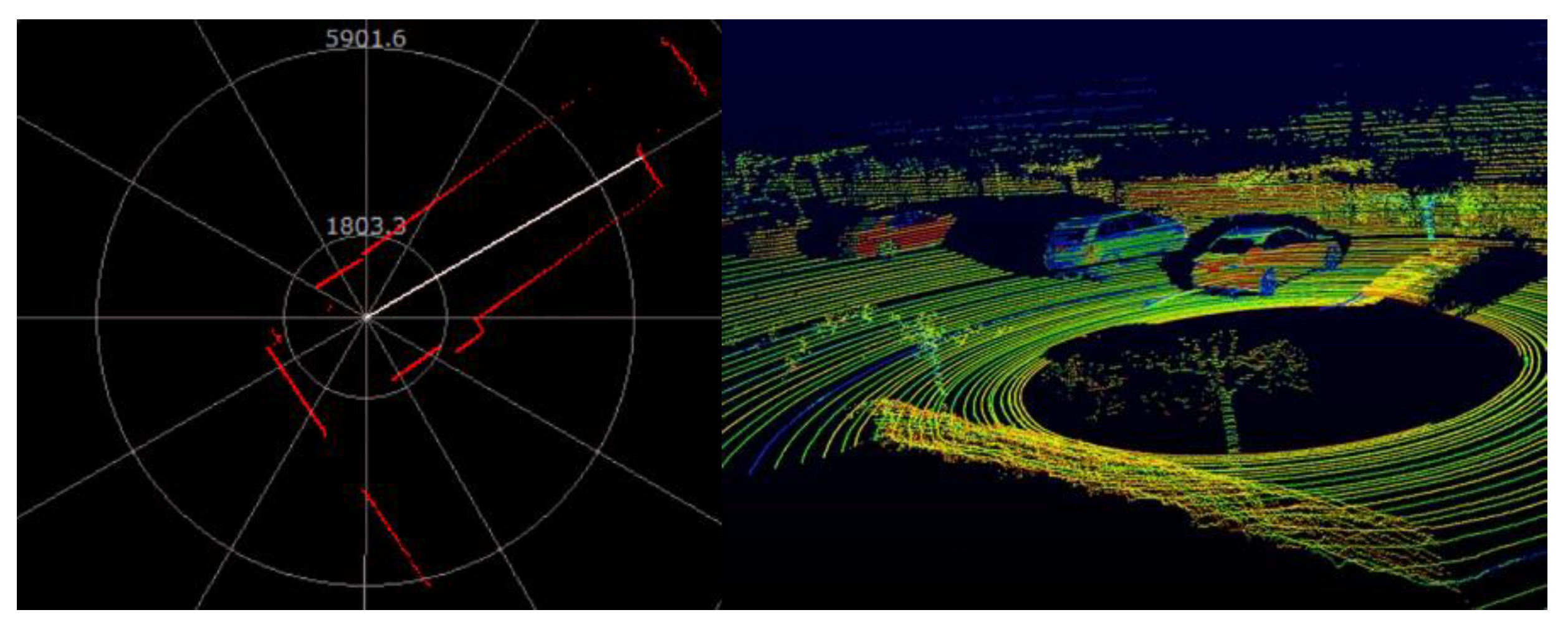
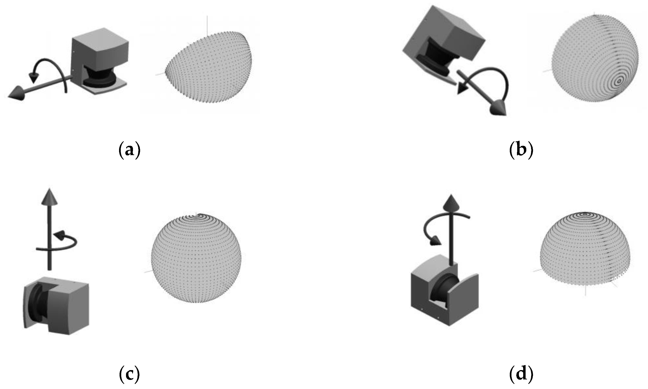
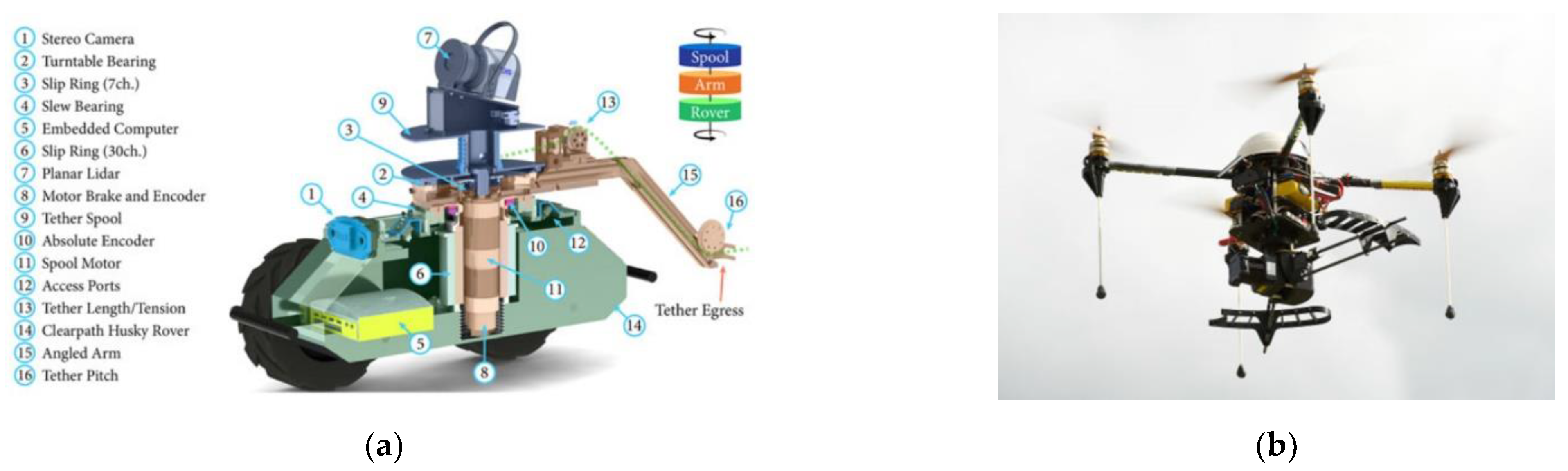
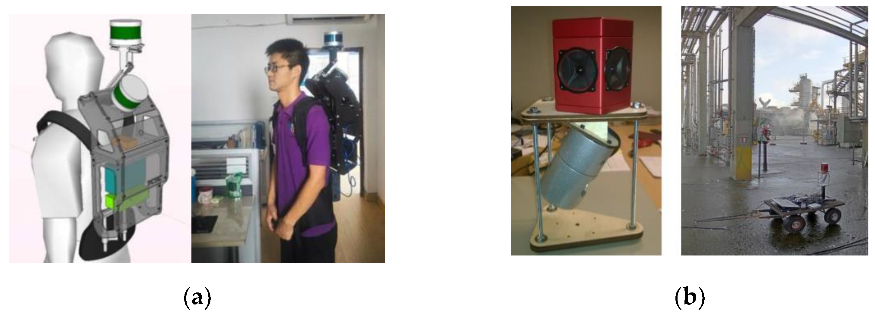
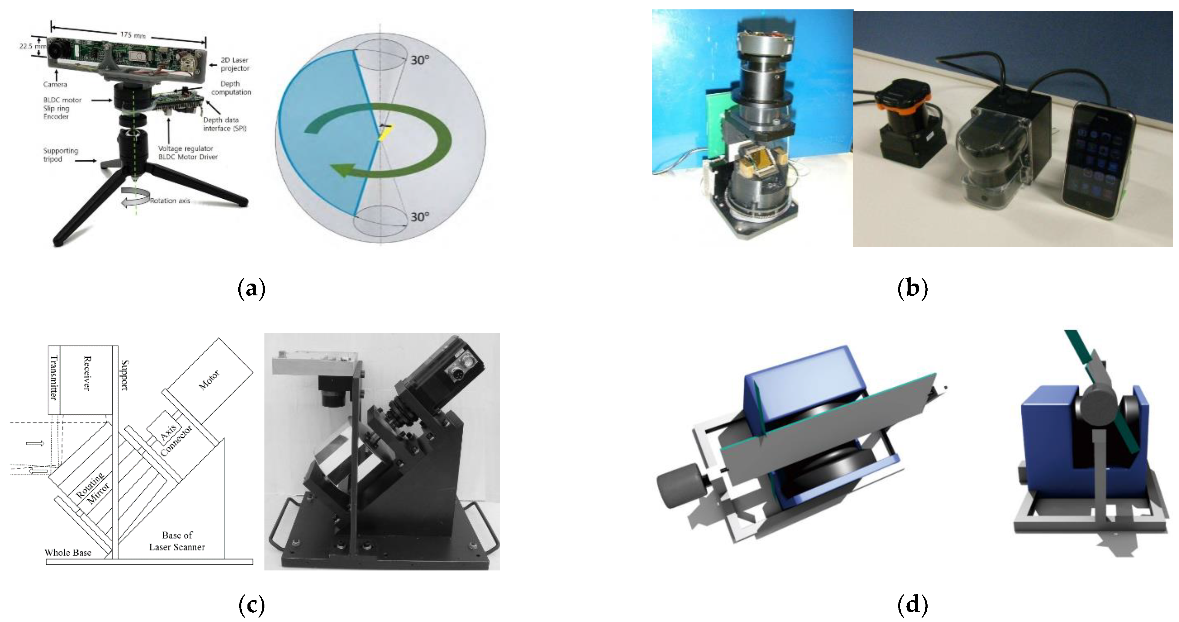
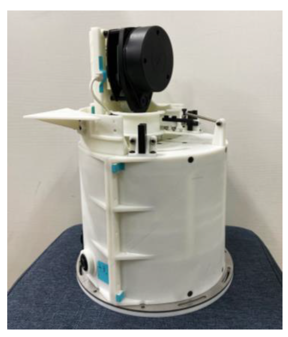
Table A1.
Representative commercial 2D LiDARs and 3D LiDARs.
| Categories | Manufacturers | Product Model ID | Performance | Prices (USD) | Application | Nations |
|---|---|---|---|---|---|---|
| 2D LiDAR | Sick | LMS111 | Single-line mechanical LiDAR, its horizontal field of vision is 270°, its measuring range is 0.5 m to 20 m, its scanning frequency is 25 Hz or 50 Hz (in different working modes), its angular resolution is 0.25° or 0.5° (in different working modes). The typical value of its systematic error is ±30 mm, and the typical value of its statistical error is 12 mm [122]. | 3813 | Outdoor; mobile robot | Germany |
| Sick | LMS511 | Single-line mechanical LiDAR, its horizontal field of vision is 190°, its measuring range is 1 m to 80 m, its scanning frequency is 25 Hz or 35 Hz or 50 Hz or 75 Hz or 100 Hz (in different working modes). Its angular resolution is 0.042° or 0.083° or 0.1667° or 0.25° or 0.333° or 0.5° or 0.667° or 1° (in different working modes). Its systematic error is ±25 mm (1 m to 10 m) or ±35 mm (10 m to 20 m) or ±50 mm (20 m to 30 m). Its statistical error is 6 mm (1 m to 10 m) or 8 mm (10 m to 20 m) or 14 mm (20 m to 30 m) [123]. | 6405 | Outdoor; mobile robot | Germany | |
| Hokuyo | UST-10LX | Single-line mechanical LiDAR, its horizontal field of vision is 270°, its measuring range is 0.06 m to 10 m, its scanning frequency is 40 Hz. Its angular resolution is 0.25°. The typical value of its accuracy is ±40 mm, and the typical value of its repeated accuracy is 30 mm [124]. | 1525 | Mobile robot | Japan | |
| Hokuyo | UTM-30LX-EW | Single-line mechanical LiDAR, its horizontal field of vision is 270°, its measuring range is 0.1 m to 10 m, its scanning frequency is 40 Hz. Its angular resolution is 0.25°. Its accuracy is ±30 mm (0.1 m to 10 m) or ±50 mm (10 m to 30 m), its repeated accuracy is 10 mm (0.1 m to 10 m) or 30 mm (10 m to 30 m) [125]. | 5338 | Mobile robot | Japan | |
| Slamtec | RPLIDAR A1 | Single-line mechanical LiDAR, its horizontal field of vision is 360°, its measuring range is 0.15 m to 12 m, its scanning frequency is 1 Hz to 10 Hz. Its angular resolution is higher than 1°. Its ranging resolution is higher than 0.5 mm or 1 percent of the measured range [6]. | 76 | Mobile robot | China | |
| Slamtec | RPLIDAR A2M6 | Single-line mechanical LiDAR, its horizontal field of vision is 360°, its measuring range is 0.2 m to 18 m, its scanning frequency is 5 Hz to 15 Hz. Its angular resolution is 0.45° to 1.35°. Its ranging resolution is higher than 0.5 mm or 1 percent of the measured range [126]. | 290 | Mobile robot | China | |
| Slamtec | RPLIDAR A3 | Single-line mechanical LiDAR, its horizontal field of vision is 360°, its measuring range is 0.2 m to 25 m, its scanning frequency is 5 Hz to 15 Hz. Its angular resolution is 0.225° or 0.36° [127]. | 625 | Mobile robot | China | |
| Slamtec | RPLIDAR S1 | Single-line mechanical LiDAR, its horizontal field of vision is 360°, its measuring range is 0.1 m to 40 m, its scanning frequency is 8 Hz to 15 Hz. Its angular resolution is 0.313° to 0.587°. Its measuring accuracy is ±50 mm, and its measuring resolution is 30 mm [128]. | 686 | Mobile robot | China | |
| Vanjee Technology | WLR-716 | Single-line mechanical LiDAR, its horizontal field of vision is 270°, its measuring range is no more than 25 m, its scanning frequency is 15 Hz. Its angular resolution is 0.33°. Its measuring accuracy is higher than ±20 mm [129]. | 991 | Mobile robot | China | |
| 3D LiDAR | Leica | BLK360 | Portable 3D laser scanner. Its horizontal field of view is 360°, and its vertical field of view is 300°. Its scanning range is 0.6 m to 60 m. Its scanning rate is as high as 360,000 points per second, and a panoramic scan can be done within 3 min. Its ranging accuracy is 4 mm (at 10 m) or 7 mm (at 20 m), and the accuracy of the constructed 3D point cloud is 6 mm (at 10 m) or 8 mm (at 20 m) [130]. | 22,875 | Surveying Engineering | Switzerland |
| Faro | FocusS Plus 350 | Terrestrial 3D laser scanner. Its horizontal field of view is 360°, and its vertical field of view is 300°. Its measuring distance is 0.6 m to 350 m, its scanning speed can be as high as 2,000,000 points per second, and the vertical and horizontal scanning steps are both 0.009°. Its ranging error is ±1 mm. Its ranging noise is 0.1 mm to 1.6 mm [131]. | 48,800 | Surveying Engineering | USA | |
| Velodyne | VLP-16 (Puck) | Sixteen lines mechanical LiDAR, with a maximum measurement range of 100 m. Its horizontal field of view is 360°, and its vertical field of view is −15° to 15°. The angular resolution in the horizontal direction is 0.1° to 0.4°, and the angular resolution in the vertical direction is 2°. Its scanning rate can be as high as 300,000 points per second, and its scanning frequency is 5 Hz to 20 Hz. The typical value of its measuring accuracy is ±3 cm [132]. | 5338 | Automatic driving | USA | |
| Velodyne | HDL-32E | Thirty-two lines mechanical LiDAR, with a maximum measurement range of 100m. Its horizontal field of view is 360°, and its vertical field of view is −30° to 10°. The angular resolution in the horizontal direction is 0.1° to 0.4°, and the angular resolution in the vertical direction is 1.33°. Its scanning rate can be as high as 700,000 points per second, and its scanning frequency is 5 Hz to 20 Hz. The typical value of its measuring accuracy is ±2 cm [133]. | 58,064 | Automatic driving | USA | |
| Velodyne | HDL-64E | Sixty-four lines mechanical LiDAR, with a maximum measurement range of 120 m. Its horizontal field of view is 360°, and its vertical field of view is −24.8° to 2°. The angular resolution in the horizontal direction is 0.08°, and the angular resolution in the vertical direction is 0.4°. Its scanning rate can be as high as 2,200,000 points per second, and its scanning frequency is 5 Hz to 20 Hz. The typical value of its measuring accuracy is ±2 cm [7]. | 103,700 | Automatic driving | USA | |
| Vanjee Technology | WLR-736 | Sixteen lines mechanical LiDAR, with a maximum measurement range of 200 m. Its horizontal field of view is 145° and its vertical field of view is 7.75°. Its horizontal angular resolution is 0.1° to 0.5°, and its vertical angular resolution is 0.56° to 0.6°. Its scanning frequency is 10 Hz or 20 Hz or 30 Hz or 40 Hz or 50 Hz (optional). Its measuring accuracy is ±6 cm [134]. | 3813 | Automatic driving | China | |
| Vanjee Technology | WLR-732 | Thirty-two lines mechanical LiDAR, with a maximum measurement range of 200 m. Its horizontal field of view is 360° and its vertical field of view is 24° (−12° to 12°). Its horizontal angular resolution is 0.1° to 0.4°, and its vertical angular resolution is 0.75°. Its scanning frequency is 5 Hz or 10 Hz or 15 Hz or 20 Hz (optional). Its measuring accuracy is ±6 cm [135]. | 16,775 | Automatic driving | China | |
| Hesai Photonics Technology | Pandar40 | Forty lines mechanical LiDAR, with a measurement range of 0.3 m to 200 m. Its horizontal field of view is 360°, and its vertical field of view is −16° to 7°. Its scanning frequency is 10 Hz or 20 Hz (optional). Its horizontal angular resolution is 0.2° or 0.4°, corresponding to the scanning frequency of 10 Hz and 20 Hz, respectively. Its vertical angle resolution is 0.33° (corresponding to the vertical field of view of −6° to 2°) or 1° (corresponding to the vertical field of view of −16° to 6° and 2° to 7°). Its measuring accuracy is ±50 mm (0.3 m to 0.5 m) or ±20 mm (0.5 m to 200 m) [136]. | 30,500 | Automatic driving | China | |
| Hesai Photonics Technology | Pandar64 | Sixty-four lines mechanical LiDAR, with a measurement range of 0.3 m to 200 m. Its horizontal field of view is 360°, and its vertical field of view is −25° to 15°. Its scanning frequency is 10 Hz or 20 Hz (optional). Its horizontal angular resolution is 0.2° or 0.4°, corresponding to the scanning frequency of 10 Hz and 20 Hz, respectively. Its minimum vertical angle resolution is 0.167°. Its measuring accuracy is ±50 mm (0.3 m to 0.5 m) or ±20 mm (0.5 m to 200 m) [137]. | 68,625 | Automatic driving | China | |
| Robosense | RS-LiDAR-16 | Sixteen lines mechanical LiDAR, with a measurement range of 0.4 m to 150 m. Its horizontal field of view is 360°, and its vertical field of view is 30°. Its horizontal angular resolution is 0.1°, 0.2°, or 0.4° (optional), and its vertical angular resolution is 2°. Its scanning frequency is 5 Hz or 10 Hz or 20 Hz (optional). Its measurement accuracy is ±20 mm [138]. | 4270 | Automatic driving | China | |
| Robosense | RS-LiDAR-32 | Thirty-two lines mechanical LiDAR, with a measurement range of 0.4 m to 200 m. Its horizontal field of view is 360°, and its vertical field of view is 40°. Its horizontal angular resolution is 0.1°, 0.2°, or 0.4° (optional), and its vertical angular resolution is 0.33°. Its scanning frequency is 5 Hz or 10 Hz or 20 Hz (optional). Its measurement accuracy is ±30 mm [139]. | 19,520 | Automatic driving | China |
It is worth mentioning that, in addition to the mechanical 3D LiDARs listed in Table A1; solid-state 3D LiDARs have been developed and commercialized successfully by some manufacturers. Different with the mechanical 3D LiDARs in which mechanical scanning method is used, phased arrays, which consist of many fixed small beam emitters, are used in solid-state 3D LiDARs. Since there are no rotating components in the solid-state 3D LiDARs, wear consumption can be avoided. Besides, compared to a mechanical 3D LiDAR, the reliability of a solid-state 3D LiDAR is greatly improved. When several beam emitters are damaged, a solid-state LiDAR can still work. Although the solid-state 3D LiDARs perform better in reliability and operational life than the mechanical 3D LiDARs, their prices tend to be higher. Since the focus of this paper is low-cost 3D laser scanning technology, the solid-state LiDARs will not be discussed in detail.
Appendix B
We have listed the notations used throughout this paper in Table A2.
Table A2.
Nomenclature.
| Symbol | Explanation |
|---|---|
| L | The coordinate frame of the 2D LiDAR. |
| L′ | The coordinate frame of the 2D LiDAR at another position. |
| W | World coordinate frame. |
| p | A sampling point of the 2D LiDAR. |
| r | The ranging data of the sampling point p. |
| θ | The azimuth angle of the sampling point p. |
| pL | The coordinate of sampling point p relative to the coordinate frame L of the 2D LiDAR. |
| pW | The coordinate of sampling point p relative to the word coordinate frame W. |
| The rotation matrix from coordinate frame L to coordinate frame W. | |
| The translation vector from coordinate frame L to coordinate frame W. | |
| P | The coordinate frame of the prototype. |
| M | The coordinate frame of the mobile platform. |
| pP | The coordinate of sampling point p relative to the coordinate frame P of the prototype. |
| The rotation matrix from coordinate frame L to coordinate frame P. | |
| The translation vector from coordinate frame L to coordinate frame P. | |
| pM | The coordinate of sampling point p relative to the coordinate frame M of the mobile platform. |
| The rotation matrix from coordinate frame P to coordinate frame M. | |
| The translation vector from coordinate frame P to coordinate frame M. | |
| The rotation matrix from coordinate frame M to coordinate frame W. | |
| The translation vector from coordinate frame M to coordinate frame W. | |
| The rotation matrix from coordinate frame L to coordinate frame M. | |
| The translation vector from coordinate frame L to coordinate frame M. |
References
- Yilmaz, V. Automated ground filtering of LiDAR and UAS point clouds with metaheuristics. Opt. Laser Technol. 2021, 138, 106890. [Google Scholar] [CrossRef]
- Jarén, R.R.; Arranz, J.J. Automatic segmentation and classification of BIM elements from point clouds. Autom. Constr. 2021, 124, 103576. [Google Scholar] [CrossRef]
- Javanmardi, E.; Javanmardi, M.; Gu, Y.; Kamijo, S. Autonomous vehicle self-localization based on multilayer 2D vector map and multi-channel LiDAR. In Proceedings of the 2017 IEEE Intelligent Vehicles Symposium (IV), Los Angeles, CA, USA, 11–14 June 2017. [Google Scholar]
- Briechle, S.; Krzystek, P.; Vosselman, G. Silvi-Net—A dual-CNN approach for combined classification of tree species and standing dead trees from remote sensing data. Int. J. Appl. Earth Obs. Geoinf. 2021, 98, 102292. [Google Scholar] [CrossRef]
- Estornell, J.; Hadas, E.; Martí, J.; López-Cortés, I. Tree extraction and estimation of walnut structure parameters using airborne LiDAR data. Int. J. Appl. Earth Obs. Geoinf. 2021, 96, 102273. [Google Scholar] [CrossRef]
- Slamtec Rplidar A1. Available online: http://www.slamtec.com/cn/Lidar/A1Spec (accessed on 20 December 2020).
- Velodyne HDL-64E. Available online: https://velodynelidar.com/products/hdl-64e/ (accessed on 13 April 2021).
- Kang, X.; Yin, S.; Fen, Y. 3D Reconstruction & Assessment Framework based on affordable 2D Lidar. In Proceedings of the 2018 IEEE/ASME International Conference on Advanced Intelligent Mechatronics (AIM), Auckland, New Zealand, 9–12 July 2018; pp. 292–297. [Google Scholar]
- Palacín, J.; Martínez, D.; Rubies, E.; Clotet, E. Mobile Robot Self-Localization with 2D Push-Broom LIDAR in a 2D Map. Sensors 2020, 20, 2500. [Google Scholar] [CrossRef]
- Morales, J.; Martínez, J.; Mandow, A.; Reina, A.; Pequenoboter, A.; García-Cerezo, A. Boresight Calibration of Construction Misalignments for 3D Scanners Built with a 2D Laser Rangefinder Rotating on Its Optical Center. Sensors 2014, 14, 20025–20040. [Google Scholar] [CrossRef] [Green Version]
- Morales, J.; Plazaleiva, V.; Mandow, A.; Gomezruiz, J.; Serón, J.; GarcíaCerezo, A. Analysis of 3D Scan Measurement Distribution with Application to a Multi-Beam Lidar on a Rotating Platform. Sensors 2018, 18, 395. [Google Scholar] [CrossRef] [PubMed] [Green Version]
- Neumann, T.; Dülberg, E.; Schiffer, S.; Ferrein, A. A Rotating Platform for Swift Acquisition of Dense 3D Point Clouds. In Proceedings of the International Conference on Intelligent Robotics and Applications, Tokyo, Japan, 22–24 August 2016; pp. 257–268. [Google Scholar]
- Pfrunder, A.; Borges, P.V.K.; Romero, A.R.; Catt, G.; Elfes, A. Real-time autonomous ground vehicle navigation in heterogeneous environments using a 3D LiDAR. In Proceedings of the 2017 IEEE/RSJ International Conference on Intelligent Robots and Systems (IROS), Vancouver, BC, Canada, 24–28 September 2017. [Google Scholar]
- Neumann, T.; Ferrein, A.; Kallweit, S.; Scholl, I. Towards a Mobile Mapping Robot for Underground Mines. In Proceedings of the 2014 PRASA, RobMech and AfLaT International Joint Symposium, Cape Town, South Africa, 27–28 November 2014. [Google Scholar]
- Mandow, A.; Morales, J.; Gomez-Ruiz, J.A.; Garcia-Cerezo, A.J. Optimizing Scan Homogeneity for Building Full-3D Lidars Based on Rotating a Multi-Beam Velodyne Range-Finder. In Proceedings of the 2018 IEEE/RSJ International Conference on Intelligent Robots and Systems (IROS), Madrid, Spain, 1–5 October 2018. [Google Scholar]
- Wen, C.; Sun, X.; Hou, S.; Tan, J.; Dai, Y.; Wang, C.; Li, J. Line Structure-Based Indoor and Outdoor Integration Using Backpacked and TLS Point Cloud Data. IEEE Geosci. Remote Sens. Lett. 2018, 15, 1790–1794. [Google Scholar] [CrossRef]
- Gong, Z.; Wen, C.; Wang, C.; Li, J. A Target-Free Automatic Self-Calibration Approach for Multibeam Laser Scanners. IEEE Trans. Instrum. Meas. 2017, 67, 238–240. [Google Scholar] [CrossRef]
- Wang, C.; Hou, S.; Wen, C.; Gong, Z.; Li, Q.; Sun, X.; Li, J. Semantic line framework-based indoor building modeling using backpacked laser scanning point cloud. ISPRS J. Photogramm. Remote Sens. 2018, 143, 150–166. [Google Scholar] [CrossRef]
- Vlaminck, M.; Luong, H.; Goeman, W.; Philips, W. 3D Scene Reconstruction Using Omnidirectional Vision and LiDAR: A Hybrid Approach. Sensors 2016, 16, 1923. [Google Scholar] [CrossRef] [Green Version]
- Alismail, H.; Browning, B. Automatic Calibration of Spinning Actuated Lidar Internal Parameters. J. Field Robot. 2015, 32, 723–747. [Google Scholar] [CrossRef]
- Kang, J.; Doh, N.L. Full-DOF Calibration of a Rotating 2-D LIDAR with a Simple Plane Measurement. IEEE Trans. Robot. 2016, 32, 1245–1263. [Google Scholar] [CrossRef]
- Gao, Z.; Huang, J.; Yang, X.; An, P. Calibration of rotating 2D LIDAR based on simple plane measurement. Sens. Rev. 2019, 39, 190–198. [Google Scholar] [CrossRef]
- Yadan, Z.; Heng, Y.; Houde, D.; Shuang, S.; Mingqiang, L.; Bo, S.; Wei, J.; Max, M. An Improved Calibration Method for a Rotating 2D LIDAR System. Sensors 2018, 18, 497. [Google Scholar]
- Martinez, J.L.; Morales, J.; Reina, A.J.; Mandow, A.; Pequeno-Boter, A.; Garcia-Cerezo, A.; IEEE. Construction and Calibration of a Low-Cost 3D Laser Scanner with 360 degrees Field of View for Mobile Robots. In Proceedings of the 2015 IEEE International Conference on Industrial Technology (ICIT), Seville, Spain, 17–19 March 2015; pp. 149–154. [Google Scholar]
- Murcia, H.F.; Monroy, M.F.; Mora, L.F. 3D Scene Reconstruction Based on a 2D Moving LiDAR. In International Conference on Applied Informatics; Springer: Cham, Switzerland, 2018. [Google Scholar]
- Petr, O.; Michal, K.; Pavel, M.; David, S. Calibration of Short Range 2D Laser Range Finder for 3D SLAM Usage. J. Sens. 2015, 2016, 1–13. [Google Scholar]
- Oberlander, J.; Pfotzer, L.; Roennau, A.; Dillmann, R. Fast calibration of rotating and swivelling 3-D laser scanners exploiting measurement redundancies. In Proceedings of the 2015 IEEE/RSJ International Conference on Intelligent Robots and Systems (IROS), Hamburg, Germany, 28 September–2 October 2015. [Google Scholar]
- Kurnianggoro, L.; Hoang, V.D.; Jo, K.H. Calibration of Rotating 2D Laser Range Finder Using Circular Path on Plane Constraints. In New Trends in Computational Collective Intelligence; Springer: Cham, Switzerland, 2015. [Google Scholar]
- Kurnianggoro, L.; Hoang, V.D.; Jo, K.H. Calibration of a 2D laser scanner system and rotating platform using a point-plane constraint. Comput. Ence. Inf. Syst. 2015, 12, 307–322. [Google Scholar] [CrossRef]
- Pfotzer, L.; Oberlaender, J.; Roennau, A.; Dillmann, R. Development and calibration of KaRoLa, a compact, high-resolution 3D laser scanner. In Proceedings of the 2014 IEEE International Symposium on Safety, Security, and Rescue Robotics (SSRR), Hokkaido, Japan, 27–30 October 2014. [Google Scholar]
- Lin, C.C.; Liao, Y.D.; Luo, W.J. Calibration method for extending single-layer LIDAR to multi-layer LIDAR. In Proceedings of the 2013 IEEE/SICE International Symposium on System Integration (SII), Honolulu, HI, USA, 12–15 January 2013. [Google Scholar]
- Choi, D.-G.; Bok, Y.; Kim, J.-S.; Kweon, I.S. Extrinsic Calibration of 2-D Lidars Using Two Orthogonal Planes. IEEE Trans. Robot. 2015, 32, 83–986. [Google Scholar] [CrossRef]
- Chen, J.; Quan, S.; Quan, Y.; Guo, Q. Calibration Method of Relative Position and Pose between Dual Two-Dimensional Laser Radar. Chin. J. Lasers 2017, 44, 152–160. [Google Scholar] [CrossRef]
- He, M.; Zhao, H.; Cui, J.; Zha, H. Calibration method for multiple 2D LIDARs system. In Proceedings of the 2014 IEEE International Conference on Robotics & Automation, Hong Kong, China, 31 May–7 June 2014. [Google Scholar]
- He, M.; Zhao, H.; Davoine, F.; Cui, J.; Zha, H. Pairwise LIDAR calibration using multi-type 3D geometric features in natural scene. In Proceedings of the 2013 IEEE/RSJ International Conference on Intelligent Robots and Systems, Tokyo, Japan, 3–7 November 2013. [Google Scholar]
- Baldwin, I.; Newman, P. Laser-only road-vehicle localization with dual 2D push-broom LIDARS and 3D priors. In Proceedings of the IEEE/RSJ International Conference on Intelligent Robots & Systems, Algarve, Portugal, 7–12 October 2012. [Google Scholar]
- Newman, P.M.; Baldwin, I. Generation of 3D Models of an Environment. U.S. Patent WO2014128498A2, 28 August 2014. Available online: https://patentimages.storage.googleapis.com/9c/d8/c3/cf9155249ecc3a/US10109104.pdf (accessed on 26 April 2021).
- Bosse, M.; Zlot, R. Continuous 3D scan-matching with a spinning 2D laser. In Proceedings of the IEEE International Conference on Robotics & Automation, Kobe, Japan, 12–17 May 2019. [Google Scholar]
- Zheng, F.; Shibo, Z.; Shiguang, W.; Yu, Z. A Real-Time 3D Perception and Reconstruction System Based on a 2D Laser Scanner. J. Sens. 2018, 2018, 1–14. [Google Scholar] [CrossRef]
- Almqvist, H.; Magnusson, M.; Lilienthal, A.J. Improving Point Cloud Accuracy Obtained from a Moving Platform for Consistent Pile Attack Pose Estimation. J. Intell. Robot. Syst. Theory Appl. 2014, 75, 101–128. [Google Scholar] [CrossRef]
- Zhang, J.; Singh, S. LOAM: Lidar Odometry and Mapping in real-time. In Proceedings of the Robotics: Science and Systems Conference (RSS), Berkeley, CA, USA, 12–16 July 2014. [Google Scholar]
- Zhang, T.; Nakamura, Y. Moving Humans Removal for Dynamic Environment Reconstruction from Slow-Scanning LIDAR Data. In Proceedings of the 2018 15th International Conference on Ubiquitous Robots (UR), Jeju, Korea, 28 June–1 July 2018. [Google Scholar]
- Kim, J.; Jeong, H.; Lee, D. Single 2D lidar based follow-me of mobile robot on hilly terrains. J. Mech. Sci. Technol. 2020, 34, 1–10. [Google Scholar]
- Dewan, A.; Caselitz, T.; Tipaldi, G.D.; Burgard, W. Motion-based detection and tracking in 3D LiDAR scans. In Proceedings of the 2016 IEEE International Conference on Robotics and Automation (ICRA), Stockholm, Sweden, 16–21 May 2016. [Google Scholar]
- Chu, P.M.; Cho, S.; Sim, S.; Kwak, K.; Park, Y.W.; Cho, K. Removing past data of dynamic objects using static Velodyne LiDAR sensor. In Proceedings of the 2016 16th International Conference on Control, Automation and Systems (ICCAS), Gyeongju, Korea, 16–19 October 2016. [Google Scholar]
- Morton, P.; Douillard, B.; Underwood, J. An evaluation of dynamic object tracking with 3D LIDAR. In Proceedings of the Australasian Conference on Robotics and Automation, Melbourne, Australia, 7–9 December 2011. [Google Scholar]
- Spinello, L.; Arras, K.O.; Triebel, R.; Siegwart, R. A Layered Approach to People Detection in 3D Range Data. In Proceedings of the Twenty-fourth Aaai Conference on Artificial Intelligence, Atlanta, GA, USA, 11–15 July 2010. [Google Scholar]
- Oliver Wulf, B.W. Fast 3D scanning methods for laser measurement systems. In Proceedings of the International Conference on Control Systems and Computer Science, CSCS14, Bucharest, Romania, 2–5 July 2003. [Google Scholar]
- Ueda, T.; Kawata, H.; Tomizawa, T.; Ohya, A.; Yuta, S.I. Mobile SOKUIKI Sensor System-Accurate Range Data Mapping System with Sensor Motion. In Proceedings of the 2006 International Conference on Autonomous Robots and Agents, Palmerston North, New Zealand, 12–14 December 2006. [Google Scholar]
- Ohno, K.; Kawahara, T.; Tadokoro, S. Development of 3D laser scanner for measuring uniform and dense 3D shapes of static objects in dynamic environment. In Proceedings of the IEEE International Conference on Robotics & Biomimetics, Guilin, China, 19–23 December 2009. [Google Scholar]
- Yoshida, T.; Irie, K.; Koyanagi, E.; Tomono, M. A sensor platform for outdoor navigation using gyro-assisted odometry and roundly-swinging 3D laser scanner. In Proceedings of the 2010 IEEE/RSJ International Conference on Intelligent Robots and Systems, Taipei, Taiwan, 18–22 October 2010. [Google Scholar]
- Matsumoto, M. 3D laser range sensor module with roundly swinging mechanism for fast and wide view range image. In Proceedings of the IEEE Conference on Multisensor Fusion and Integration, Salt Lake City, UT, USA, 5–7 September 2010. [Google Scholar]
- Schubert, S.; Neubert, P.; Protzel, P. How to Build and Customize a High-Resolution 3D Laserscanner Using Off-the-shelf Components. In Proceedings of the Conference towards Autonomous Robotic Systems, Sheffield, UK, 26 June–1 July 2016. [Google Scholar]
- Ocando, M.G.; Certad, N.; Alvarado, S.; Terrones, N. Autonomous 2D SLAM and 3D mapping of an environment using a single 2D LIDAR and ROS. In Proceedings of the 2017 Latin American Robotics Symposium (LARS) and 2017 Brazilian Symposium on Robotics (SBR), Curitiba, Brazil, 8–10 November 2017. [Google Scholar]
- Wu, Q.; Sun, K.; Zhang, W.; Huang, C.; Wu, X. Visual and LiDAR-based for the mobile 3D mapping. In Proceedings of the IEEE International Conference on Robotics & Biomimetics, Qingdao, China, 3–7 December 2016. [Google Scholar]
- Brenneke, C.; Wulf, O.; Wagner, B. Using 3D Laser Range Data for SLAM in Outdoor Environments. In Proceedings of the 2003 IEEE/RSJ International Conference on Intelligent Robots and Systems (IROS 2003), Las Vegas, NV, USA, 27–31 October 2003. [Google Scholar]
- Wen, C.; Qin, L.; Zhu, Q.; Wang, C. Three-Dimensional Indoor Mobile Mapping with Fusion of Two-Dimensional Laser Scanner and RGB-D Camera Data. IEEE Geosci. Remote Sens. Lett. 2013, 11, 843–847. [Google Scholar]
- Cong, P.; Xunyu, Z.; Huosheng, H.; Jun, T.; Xiafu, P.; Jianping, Z. Adaptive Obstacle Detection for Mobile Robots in Urban Environments Using Downward-Looking 2D LiDAR. Sensors 2018, 18, 1749. [Google Scholar]
- Demir, S.O.; Ertop, T.E.; Koku, A.B.; Konukseven, E.I. An adaptive approach for road boundary detection using 2D LIDAR sensor. In Proceedings of the 2017 IEEE International Conference on Multisensor Fusion and Integration for Intelligent Systems (MFI), Daegu, Korea, 16–18 November 2017. [Google Scholar]
- Xu, W.; Zhuang, Y.; Hu, H.; Zhao, Y. Real-time road detection and description for robot navigation in an unstructured campus environment. In Proceedings of the 11th World Congress on Intelligent Control and Automation, Shenyang, China, 29 June–4 July 2014. [Google Scholar]
- Wang, X.; Cai, Y.; Shi, T. Road edge detection based on improved RANSAC and 2D LIDAR Data. In Proceedings of the International Conference on Control, Jeju Island, Korea, 25–28 November 2015. [Google Scholar]
- Dias, P.; Matos, M.; Santos, V. 3D Reconstruction of Real World Scenes Using a Low-Cost 3D Range Scanner. Comput. Aided Civil. Infrastruct. Eng. 2010, 21, 486–497. [Google Scholar] [CrossRef]
- Li, J.; He, X.; Li, J. 2D LiDAR and Camera Fusion in 3D Modeling of Indoor Environment. In Proceedings of the 2015 National Aerospace and Electronics Conference (NAECON), Penang, Malaysia, 27–29 November 2015. [Google Scholar]
- Wang, S.; Zhuang, Y.; Zheng, K.; Wang, W. 3D Scene Reconstruction Using Panoramic Laser Scanning and Monocular Vision. In Proceedings of the 2010 8th World Congress on Intelligent Control and Automation, Jinan, China, 7–9 July 2010. [Google Scholar]
- Alismail, H.; Baker, L.D.; Browning, B. Automatic Calibration of a Range Sensor and Camera System. In Proceedings of the 2012 Second International Conference on 3D Imaging, Modeling, Processing, Visualization & Transmission, Zurich, Switzerland, 13–15 October 2012. [Google Scholar]
- Scaramuzza, D.; Harati, A.; Siegwart, R. Extrinsic self calibration of a camera and a 3D laser range finder from natural scenes. In Proceedings of the IEEE/RSJ International Conference on Intelligent Robots & Systems, San Diego, CA, USA, 29 October–2 November 2007. [Google Scholar]
- Shaukat, A.; Blacker, P.; Spiteri, C.; Gao, Y. Towards Camera-LIDAR Fusion-Based Terrain Modelling for Planetary Surfaces: Review and Analysis. Sensors 2016, 11, 1952. [Google Scholar] [CrossRef] [Green Version]
- Weingarten, J.W.; Siegwart, R. 3D SLAM using planar segments. In Proceedings of the IEEE/RSJ International Conference on Intelligent Robots & Systems, Beijing, China, 9–15 October 2006. [Google Scholar]
- Morales, J.; Martinez, J.L.; Mandow, A.; Pequenoboter, A.; Garciacerezo, A. Design and development of a fast and precise low-cost 3D laser rangefinder. In Proceedings of the International Conference on Mechatronics, Beijing, China, 7–10 August 2011; pp. 621–626. [Google Scholar]
- Baldwin, I.; Newman, P. Road vehicle localization with 2D push-broom LIDAR and 3D priors. In Proceedings of the 2012 IEEE International Conference on Robotics and Automation, Saint Paul, MN, USA, 14–18 May 2012. [Google Scholar]
- Napier, A.; Corke, P.; Newman, P. Cross-calibration of push-broom 2D LIDARs and cameras in natural scenes. In Proceedings of the 2013 IEEE International Conference on Robotics and Automation, Karlsruhe, Germany, 6–10 May 2013. [Google Scholar]
- Wen, C.; Pan, S.; Wang, C.; Li, J. An Indoor Backpack System for 2-D and 3-D Mapping of Building Interiors. IEEE Geosci. Remote Sens. Lett. 2016, 13, 992–996. [Google Scholar] [CrossRef]
- Liu, T.; Carlberg, M.; Chen, G.; Chen, J.; Zakhor, A. Indoor localization and visualization using a human-operated backpack system. In Proceedings of the 2010 International Conference on Indoor Positioning and Indoor Navigation, Zurich, Switzerland, 15–17 September 2010. [Google Scholar]
- Bok, Y.; Choi, D.; Jeong, Y.; Kweon, I.S. Capturing village-level heritages with a hand-held camera-laser fusion sensor. In Proceedings of the IEEE International Conference on Computer Vision Workshops, Barcelona, Spain, 6–13 November 2011. [Google Scholar]
- Dong-Geol, C.; Yunsu, B.; Jun-Sik, K.; Inwook, S.; In, K. Structure-From-Motion in 3D Space Using 2D Lidars. Sensors 2017, 17, 242. [Google Scholar]
- Winkvist, S.; Rushforth, E.; Young, K. Towards an autonomous indoor aerial inspection vehicle. Ind. Robot. 2013, 40, 196–207. [Google Scholar] [CrossRef]
- Wang, A.; Li, C.; Liu, Y.; Zhuang, Y.; Bu, C.; Xiao, J. Laser-based Online Sliding-window Approach for UAV Loop-closure Detection in Urban Environments. Int. J. Adv. Robot. Syst. 2017, 13, 1–11. [Google Scholar] [CrossRef]
- Mcgarey, P.; Yoon, D.; Tang, T.; Pomerleau, F.; Barfoot, T.D. Developing and deploying a tethered robot to map extremely steep terrain: MCGAREY et al. J. Field Robot. 2018, 35, 1327–1341. [Google Scholar] [CrossRef]
- Kaul, L.; Zlot, R.; Bosse, M. Continuous-Time Three-Dimensional Mapping for Micro Aerial Vehicles with a Passively Actuated Rotating Laser Scanner. J. Field Robot. 2015, 33, 103–132. [Google Scholar] [CrossRef]
- Bosse, M.; Zlot, R.; Flick, P. Zebedee: Design of a Spring-Mounted 3-D Range Sensor with Application to Mobile Mapping. IEEE Trans. Robot. 2012, 28, 1104–1119. [Google Scholar] [CrossRef]
- Bosse, M.; Zlot, R. Place recognition using keypoint voting in large 3D lidar datasets. In Proceedings of the IEEE International Conference on Robotics & Automation, Karlsruhe, Germany, 6–10 May 2013. [Google Scholar]
- Leica. Available online: https://shop.leica-geosystems.com/ (accessed on 12 April 2021).
- Faro. Available online: https://www.faro.com/ (accessed on 26 April 2021).
- Velodyne. Available online: https://velodynelidar.com/ (accessed on 12 April 2021).
- Desai, A.; Huber, D. Objective Evaluation of Scanning Ladar Configurations for Mobile Robots. In Proceedings of the IEEE/RSJ International Conference on Intelligent Robots & Systems, St. Louis, MO, USA, 11–15 October 2009. [Google Scholar]
- Son, Y.; Yoon, S.; Oh, S.Y.; Han, S. A Lightweight and Cost-Effective 3D Omnidirectional Depth Sensor Based on Laser Triangulation. IEEE Access 2019, 7, 58740–58750. [Google Scholar] [CrossRef]
- Kimoto, K.; Asada, N.; Mori, T.; Hara, Y.; Yuta, S.I. Development of small size 3D LIDAR. In Proceedings of the IEEE International Conference on Robotics & Automation, Hong Kong, China, 31 May–5 June 2014. [Google Scholar]
- Hu, C.; Huang, Z.; Qin, S. A New 3D Imaging Lidar Based on the High-Speed 2D Laser Scanner; SPIE—The International Society for Optical Engineering: Bellingham, WA, USA, 2012. [Google Scholar]
- Ryde, J.; Hu, H. Mobile Robot 3D Perception and Mapping without Odometry Using Multi-Resolution Occupancy Lists. In Proceedings of the 2007 International Conference on Mechatronics and Automation, Harbin, China, 5–9 August 2007; pp. 331–336. [Google Scholar]
- Park, C.S.; Kim, D.; You, B.J.; Oh, S.R. Characterization of the Hokuyo UBG-04LX-F01 2D laser rangefinder. In Proceedings of the 19th International Symposium in Robot and Human Interactive Communication, Viareggio, Italy, 13–15 September 2010. [Google Scholar]
- Okubo, Y.; Ye, C.; Borenstein, J. Characterization of the Hokuyo URG-04LX laser rangefinder for mobile robot obstacle negotiation. Proc. SPIE Int. Soc. Opt. Eng. 2009, 7332, 733212. [Google Scholar]
- Ueda, T.; Kawata, H.; Tomizawa, T.; Ohya, A.; Yuta, S.I. Visual Information Assist System Using 3D SOKUIKI Sensor for Blind People, System Concept and Object Detecting Experiments. In Proceedings of the Conference of the IEEE Industrial Electronics Society, Paris, France, 7–10 November 2006. [Google Scholar]
- Raymond, S.; Nawid, J.; Mohammed, K.; Claude, S. A Low-Cost, Compact, Lightweight 3D Range Sensor. In Proceedings of the Australian Conference on Robotics and Automation, Auckland, New Zealand, 6–8 December 2006. [Google Scholar]
- Matsumoto, M.; Yuta, S. 3D SOKUIKI sensor module with roundly swinging mechanism for taking wide-field range and reflection intensity image in high speed. In Proceedings of the IEEE International Conference on Robotics and Biomimetics, Phuket, Thailand, 7–11 December 2011. [Google Scholar]
- Nasrollahi, M.; Bolourian, N.; Zhu, Z.; Hammad, A. Designing LiDAR-equipped UAV Platform for Structural Inspection. In Proceedings of the 34th International Symposium on Automation and Robotics in Construction, Taipei, Taiwan, 27–30 June 2017. [Google Scholar]
- Nagatani, K.; Tokunaga, N.; Okada, Y.; Yoshida, K. Continuous Acquisition of Three-Dimensional Environment Information for Tracked Vehicles on Uneven Terrain. In Proceedings of the IEEE International Workshop on Safety, Sendai, Japan, 21–24 October 2008. [Google Scholar]
- Walther, M.; Steinhaus, P.; Dillmann, R. A foveal 3D laser scanner integrating texture into range data. In Proceedings of the International Conference on Intelligent Autonomous Systems 9-ias, Tokyo, Japan, 7–9 March 2006. [Google Scholar]
- Bertussi, S. Spin_Hokuyo—ROS Wiki. Available online: http://wiki.ros.org/spin_hokuyo (accessed on 13 February 2021).
- Yuan, C.; Bi, S.; Cheng, J.; Yang, D.; Wang, W. Low-Cost Calibration of Matching Error between Lidar and Motor for a Rotating 2D Lidar. Appl. Sci. 2021, 11, 913. [Google Scholar] [CrossRef]
- Ozbay, B.; Kuzucu, E.; Gul, M.; Ozturk, D.; Tasci, M.; Arisoy, A.M.; Sirin, H.O.; Uyanik, I. A high frequency 3D LiDAR with enhanced measurement density via Papoulis-Gerchberg. In Proceedings of the 2015 International Conference on Advanced Robotics (ICAR), Istanbul, Turkey, 27–31 July 2015; pp. 543–548. [Google Scholar]
- Kuzucu, E.; Öztürk, D.; Gül, M.; Özbay, B.; Arisoy, A.M.; Sirin, H.O.; Uyanik, I. Enhancing 3D range image measurement density via dynamic Papoulis–Gerchberg algorithm. Trans. Inst. Meas. Control 2018, 40, 4407–4420. [Google Scholar] [CrossRef]
- Yang, D.; Bi, S.; Wang, W.; Qi, X.; Cai, Y. DRE-SLAM: Dynamic RGB-D Encoder SLAM for a Differential-Drive Robot. Remote Sens. 2019, 11, 380. [Google Scholar] [CrossRef] [Green Version]
- YOLO. Available online: https://pjreddie.com/darknet/yolo/ (accessed on 16 February 2021).
- Li, Q.; Dai, B.; Fu, H. LIDAR-based dynamic environment modeling and tracking using particles based occupancy grid. In Proceedings of the 2016 IEEE International Conference on Mechatronics and Automation, Harbin, China, 7–10 August 2016. [Google Scholar]
- Qin, B.; Chong, Z.J.; Soh, S.H.; Bandyopadhyay, T.; Ang, M.H.; Frazzoli, E.; Rus, D. A Spatial-Temporal Approach for Moving Object Recognition with 2D LIDAR. In Experimental Robotics; Springer: Cham, Switzerland, 2016. [Google Scholar]
- Wang, D.Z.; Posner, I.; Newman, P. Model-free detection and tracking of dynamic objects with 2D lidar. Int. J. Robot. Res. 2015, 34, 1039–1063. [Google Scholar] [CrossRef]
- Park, Y.; Yun, S.; Won, C.; Cho, K.; Um, K.; Sim, S. Calibration between Color Camera and 3D LIDAR Instruments with a Polygonal Planar Board. Sensors 2014, 14, 5333–5353. [Google Scholar] [CrossRef] [Green Version]
- Gong, X.; Lin, Y.; Liu, J. 3D LIDAR-Camera Extrinsic Calibration Using an Arbitrary Trihedron. Sensors 2013, 12, 1902–1918. [Google Scholar] [CrossRef] [Green Version]
- Mirzaei, F.M.; Kottas, D.G.; Roumeliotis, S.I. 3D LIDAR–camera intrinsic and extrinsic calibration: Identifiability and analytical least-squares-based initialization. Int. J. Robot. Res. 2012, 31, 452–467. [Google Scholar] [CrossRef] [Green Version]
- Zhou, L.; Li, Z.; Kaess, M. Automatic Extrinsic Calibration of a Camera and a 3D LiDAR using Line and Plane Correspondences. In Proceedings of the IEEE/RSJ International Conference on Intelligent Robots & Systems, Madrid, Spain, 30 October–5 November 2018. [Google Scholar]
- Fremont, V.; Bonnifait, P. Extrinsic calibration between a multi-layer lidar and a camera. In Proceedings of the IEEE International Conference on Multisensor Fusion and Integration for Intelligent Systems, Seoul, Korea, 20–22 August 2008. [Google Scholar]
- Zhou, L.; Deng, Z. Extrinsic calibration of a camera and a lidar based on decoupling the rotation from the translation. In Proceedings of the Intelligent Vehicles Symposium, Alcalá de Henares, Spain, 3–7 June 2012. [Google Scholar]
- Weimin, W.; Ken, S.; Nobuo, K. Reflectance Intensity Assisted Automatic and Accurate Extrinsic Calibration of 3D LiDAR and Panoramic Camera Using a Printed Chessboard. Remote Sens. 2017, 9, 851. [Google Scholar]
- Hokuyo. Available online: https://www.hokuyo-aut.co.jp/ (accessed on 12 April 2021).
- Slamtec. Available online: http://www.slamtec.com/ (accessed on 12 April 2021).
- Riegl. Available online: http://www.riegl.com/ (accessed on 12 April 2021).
- Barbarella, M.; De Blasiis, M.R.; Fiani, M. Terrestrial laser scanner for the analysis of airport pavement geometry. Int. J. Pavement Eng. 2018, 20, 466–480. [Google Scholar] [CrossRef]
- Barbarella, M.; D’Amico, F.; De Blasiis, M.R.; Di Benedetto, A.; Fiani, M. Use of Terrestrial Laser Scanner for Rigid Airport Pavement Management. Sensors 2018, 18, 44. [Google Scholar] [CrossRef] [PubMed] [Green Version]
- Blasiis, M.D.; Benedetto, A.D.; Fiani, M.; Garozzo, M. Assessing of the Road Pavement Roughness by Means of LiDAR Technology. Coatings 2021, 11, 17. [Google Scholar] [CrossRef]
- De Giglio, M.; Greggio, N.; Goffo, F.; Merloni, N.; Dubbini, M.; Barbarella, M. Comparison of Pixel- and Object-Based Classification Methods of Unmanned Aerial Vehicle Data Applied to Coastal Dune Vegetation Communities: Casal Borsetti Case Study. Remote Sens. 2019, 11, 1416. [Google Scholar] [CrossRef] [Green Version]
- Barbarella, M.; Fiani, L. Application of Lidar-Derived Dem for Detection of Mass Movements on a Landslide. ISPRS Int. Arch. Photogramm. Remote Sens. Spat. Inf. Sci. 2014, 1, 159–165. [Google Scholar] [CrossRef] [Green Version]
- SICK LMS111. Available online: https://www.sick.com/ag/en/detection-and-ranging-solutions/2d-lidar-sensors/lms1xx/lms111-10100/p/p109842 (accessed on 13 April 2021).
- SICK LMS511. Available online: https://www.sick.com/ag/en/detection-and-ranging-solutions/2d-lidar-sensors/lms5xx/lms511-10100-pro/p/p215941 (accessed on 13 April 2021).
- Hokuyo UST-10LX. Available online: https://www.hokuyo-aut.co.jp/search/single.php?serial=16 (accessed on 12 November 2020).
- UTM-30LX-EW. Available online: https://www.hokuyo-aut.jp/search/single.php?serial=170 (accessed on 26 April 2021).
- Slamtec Rplidar A2M6. Available online: http://www.slamtec.com/cn/Lidar/A2Spec (accessed on 12 April 2021).
- Slamtec Rplidar A3. Available online: http://www.slamtec.com/cn/Lidar/A3Spec (accessed on 12 April 2021).
- Slamtec Rplidar S1. Available online: http://www.slamtec.com/cn/Lidar/S1Spec (accessed on 12 April 2021).
- Vanjee Technology WLR-716. Available online: http://wanji.net.cn/index.php?m=content&c=index&a=show&catid=110&id=123 (accessed on 12 April 2021).
- Leica BLK360. Available online: https://shop.leica-geosystems.com/blk360-scanner (accessed on 12 April 2021).
- Faro FocusS Plus 350. Available online: https://www.faro.com/zh-CN/Resource-Library/Tech-Sheet/techsheet-faro-focus-laser-scanners (accessed on 26 April 2021).
- Velodyne VLP-16 (Puck). Available online: https://velodynelidar.com/products/puck/ (accessed on 13 April 2021).
- Velodyne HDL-32E. Available online: https://velodynelidar.com/products/hdl-32e/ (accessed on 13 April 2021).
- Vanjee Technology WLR-736. Available online: http://wanji.net.cn/index.php?m=content&c=index&a=show&catid=99&id=86 (accessed on 13 April 2021).
- Vanjee Technology WLR-732. Available online: http://wanji.net.cn/index.php?m=content&c=index&a=show&catid=99&id=87 (accessed on 13 April 2021).
- Hesai Photonics Technology Pandar40. Available online: https://www.hesaitech.com/zh/Pandar40 (accessed on 13 April 2021).
- Hesai Photonics Technology Pandar64. Available online: https://www.hesaitech.com/zh/Pandar64 (accessed on 13 April 2021).
- Robosense RS-LiDAR-16. Available online: https://www.robosense.cn/rslidar/rs-lidar-16 (accessed on 13 April 2021).
- Robosense RS-LiDAR-32. Available online: https://www.robosense.cn/rslidar/RS-LiDAR-32 (accessed on 13 April 2021).
Figure 1.
Left: map built by 2D LiDAR Slamtec RPLIDAR A1 [6]. Right: map built by 3D LiDAR Velodyne HDL-64E [7].

Figure 2.
The principle of a moving 2D LiDAR.

Figure 3.
A pitching 2D LiDAR (left) and a rotating 2D LiDAR (right) [69].
Figure 3.
A pitching 2D LiDAR (left) and a rotating 2D LiDAR (right) [69].

Figure 4.
A rotating 2D LiDAR and a pitching 2D LiDAR in different attitudes. (a) A pitching 2D LiDAR whose rotation axis is horizontal; (b) a rotating 2D LiDAR whose rotation axis is horizontal; (c) a pitching 2D LiDAR whose rotation axis is vertical; (d) a rotating 2D LiDAR whose rotation axis is vertical [48].

Figure 5.
A rotating 2D LiDAR and a pitching 2D LiDAR. (a) A pitching 2D LiDAR mounted on a mobile platform. Left: the prototype in [68]; right: the pitching scanning example in [68]; (b) the prototype in [38], a rotating 2D LiDAR (circled in red) which is mounted on a skid-steer loader; (c) the prototype in [20], which is a rotating 2D LiDAR; (d) the prototype in [69], which is a pitching 2D LiDAR; (e) the prototypes in [48]. Left: the first-generation prototype, which is a pitching 2D LiDAR whose rotation axis is vertical; right: the second-generation prototype, which is a rotating 2D LiDAR. Compared with the first-generation prototype, in the second-generation prototype a slip ring has been used, so that the 2D LiDAR can be rotated endlessly, without being blocked by cables.

Figure 6.
Push-broom 2D LiDARs carried by different platforms. (a) A push-broom 2D LiDAR mounted on a vehicle. Left: the experimental platform in [36]; right: the push-broom scanning example in [71]; (b) push-broom 2D LiDARs mounted on a backpack. Left: the prototype in [72]; right: the 3D model of the prototype in [73]; (c) handheld push-broom 2D LiDARs. Left: the prototype in [74]; right: the prototype in [75]; (d) UAV-mounted push-broom 2D LiDARs. Left: the prototype in [76]; right: the prototype in [77].

Figure 7.
An irregularly rotating 2D LiDAR, the 2D LiDAR rotates irregularly. (a) The prototype in [78]; (b) the prototype in [79].

Figure 8.
An obliquely rotating 2D LiDAR, the 2D LiDAR is rotated periodically and is mounted obliquely. The distribution of the 3D point cloud built by an obliquely rotating 2D LiDAR is a set of grid-like lines. (a) The prototype in [50]; (b) the prototype in [51]; (c) the prototype in [52]; (d) the prototype in [53].


Figure 9.
An irregularly moving 2D LiDAR, the movement of the 2D LiDAR is irregular. The prototype in [80,81] is called Zebedee. From this figure we can see the main components of Zebedee—that is, a 2D LiDAR, an IMU, a spring and a handhold pole.

Figure 10.
A rotating 3D LiDAR and a pitching 3D LiDAR. (a) The prototype in [12]; (b) left: the prototype in [13]; right: the prototype (in the red circle) is mounted on an unmanned vehicle, the blue circles and the purple dot represent the 2D LiDARs and the rear wheel encoder respectively; (c) the prototype in [14]; (d) the prototype in [11], left: side view; right: front view.


Figure 11.
A push-broom 3D LiDAR. (a) The prototype in [16,17,18]; (b) left: the prototype in [19], in which the red device mounted above is a ladybug panoramic camera, it is used to perceive colors. The silver-white device mounted obliquely below is a 32-line 3D LiDAR Velodyne HDL-32e; right: the prototype is carried by a trolley.

Figure 12.
The prototypes in [86,87,88,89]. (a) Left: the prototype in [86]; right: the field of view of this prototype; (b) the prototypes in [87]. Left: the first-generation prototype; right: the second-generation prototype, it is placed between a commercial 2D LiDAR and a mobile phone to show its size; (c) the prototype in [88]; (d) the prototype in [89].

Figure 13.
The conversions of the coordinates of the sampling points in a rotating 2D LiDAR and a push-broom 2D LiDAR respectively. Left: a rotating 2D LiDAR is mounted on a mobile platform; right: a 2D LiDAR is fixedly mounted on a mobile platform, making it a push-broom 2D LiDAR.
Figure 13.
The conversions of the coordinates of the sampling points in a rotating 2D LiDAR and a push-broom 2D LiDAR respectively. Left: a rotating 2D LiDAR is mounted on a mobile platform; right: a 2D LiDAR is fixedly mounted on a mobile platform, making it a push-broom 2D LiDAR.

Figure 14.
The prototype built by us, which is a low-cost 3D laser scanner.

Table 1.
Classification of the prototypes.
| Serial Numbers | Categories | The Movement of 2D LiDAR | Characteristics |
|---|---|---|---|
| 1 | A rotating 2D LiDAR |  | The 2D LiDAR is rotated regularly around the middle line of the scanning sector [20,38,48]. |
| 2 | A pitching 2D LiDAR |  | The 2D LiDAR is rotated regularly around the perpendicular of the middle line of the scanning sector [68,69]. |
| 3 | A push-broom 2D LiDAR |  | The 2D LiDAR is fixedly assembled on the mobile platform [16,36,37,70,71,72,73,74,75,76,77]. |
| 4 | An irregularly rotating 2D LiDAR |  | The rotation of the 2D LiDAR is non-periodic and irregular [78,79]. |
| 5 | An obliquely rotating 2D LiDAR |  | The 2D LiDAR is rotated obliquely so that the distribution of the collected 3D point cloud is grid-like [50,51,52,53]. |
| 6 | An irregularly moving 2D LiDAR |  | The movement of the 2D LiDAR is irregular and is recorded by an IMU (inertial measurement unit) [80,81]. |
Note: for a moving 2D LiDAR, the above six categories cover most of the prototypes. There may also be some derived categories. Generally, a derived category is similar to one of the above six categories.
Table 2.
The problems of a moving 2D LiDAR.
| Problems | Categories of Problems | Categories of Prototypes | |||||
|---|---|---|---|---|---|---|---|
| 1 | 2 | 3 | 4 | 5 | 6 | ||
| Problem 1.1. The measurement error of the 2D LiDAR. | Accuracy | • | • | • | • | • | • |
| Problem 1.2. The error caused by the motor. | • | • | • | ||||
| Problem 1.3. The error caused by the assembly inaccuracy between the 2D LiDAR and the rotating unit. | • | • | • | • | |||
| Problem 1.4. The error caused by the synchronization inaccuracy between the 2D LiDAR and the rotating unit. | • | • | • | ||||
| Problem 1.5. The error caused by the assembly inaccuracy between a moving 2D LiDAR and the mobile platform. | • | • | • | • | • | • | |
| Problem 1.6. The error caused by the estimation inaccuracy of the movement of the mobile platform. | • | • | • | • | • | • | |
| Problem 2.1. The negative correlation between the real-time performance and the density of the 3D point cloud. | Real-time performance | • | • | • | • | • | • |
| Problem 2.2. The distortion of the 3D point cloud caused by the movement of the mobile platform. | • | • | • | • | |||
| Problem 2.3. The distortion of the 3D point cloud caused by the moving objects in the environment. | • | • | • | • | • | • | |
| Problem 3.1. The density distribution of the 3D point cloud built by a moving 2D LiDAR. | Others | • | • | • | • | • | • |
| Problem 3.2. The fusion of a moving 2D LiDAR and 2D LiDAR SLAM. | • | • | • | • | • | • | |
| Problem 3.3. A push-broom 2D LiDAR, which is used for the detection of the obstacles in front of the vehicle. | • | ||||||
| Problem 3.4. The fusion of a moving 2D LiDAR and a camera. | • | • | • | • | • | • | |
Note: the six categories of prototypes in Table 2 are (1) a rotating 2D LiDAR, (2) a pitching 2D LiDAR, (3) a push-broom 2D LiDAR, 4) an irregularly rotating 2D LiDAR, (5) an obliquely rotating 2D LiDAR, and (6) an irregularly moving 2D LiDAR, respectively.
Publisher’s Note: MDPI stays neutral with regard to jurisdictional claims in published maps and institutional affiliations. |
© 2021 by the authors. Licensee MDPI, Basel, Switzerland. This article is an open access article distributed under the terms and conditions of the Creative Commons Attribution (CC BY) license (https://creativecommons.org/licenses/by/4.0/).
Share and Cite
MDPI and ACS Style
Bi, S.; Yuan, C.; Liu, C.; Cheng, J.; Wang, W.; Cai, Y. A Survey of Low-Cost 3D Laser Scanning Technology. Appl. Sci. 2021, 11, 3938. https://0-doi-org.brum.beds.ac.uk/10.3390/app11093938
AMA Style
Bi S, Yuan C, Liu C, Cheng J, Wang W, Cai Y. A Survey of Low-Cost 3D Laser Scanning Technology. Applied Sciences. 2021; 11(9):3938. https://0-doi-org.brum.beds.ac.uk/10.3390/app11093938
Chicago/Turabian StyleBi, Shusheng, Chang Yuan, Chang Liu, Jun Cheng, Wei Wang, and Yueri Cai. 2021. "A Survey of Low-Cost 3D Laser Scanning Technology" Applied Sciences 11, no. 9: 3938. https://0-doi-org.brum.beds.ac.uk/10.3390/app11093938
Note that from the first issue of 2016, this journal uses article numbers instead of page numbers. See further details here.