A Whole-Slide Image Managing Library Based on Fastai for Deep Learning in the Context of Histopathology: Two Use-Cases Explained

Abstract

Background: Processing whole-slide images (WSI) to train neural networks can be intricate and labor intensive. We developed an open-source library dealing with recurrent tasks in the processing of WSI and helping with the training and evaluation of neuronal networks for classification tasks. Methods: Two histopathology use-cases were selected and only hematoxylin and eosin (H&E) stained slides were used. The first use case was a two-class classification problem. We trained a convolutional neuronal network (CNN) to distinguish between dysembryoplastic neuroepithelial tumor (DNET) and ganglioglioma (GG), two neuropathological low-grade epilepsy-associated tumor entities. Within the second use case, we included four clinicopathological disease conditions in a multilabel approach. Here we trained a CNN to predict the hormone expression profile of pituitary adenomas. In the same approach, we also predicted clinically silent corticotroph adenoma. Results: Our DNET-GG classifier achieved an AUC of 1.00 for the ROC curve. For the second use case, the best performing CNN achieved an area under the curve (AUC) of 0.97 for the receiver operating characteristic (ROC) for corticotroph adenoma, 0.86 for silent corticotroph adenoma, and 0.98 for gonadotroph adenoma. All scores were calculated with the help of our library on predictions on a case basis. Conclusions: Our comprehensive and fastai-compatible library is helpful to standardize the workflow and minimize the burden of training a CNN. Indeed, our trained CNNs extracted neuropathologically relevant information from the WSI. This approach will supplement the clinicopathological diagnosis of brain tumors, which is currently based on cost-intensive microscopic examination and variable panels of immunohistochemical stainings.

1. Introduction

With the increasing availability of digital microscopy scanners and whole slide imaging, digital pathology (DP) will continue to successfully grow into our daily routine diagnostic practice. Whole-slide images, as they are digitized slides, provide the intriguing opportunity for the application of image analysis techniques for advanced tasks, such as disease classification. Deep learning (DL) is the most commonly applied technology in the realm of feature learning. The process involves the iterative improvement of learned representations of regions of interest to achieve maximum class separability. Medical (and nonmedical) image classification tasks have been remarkably successful utilizing DL. The area of computational image analysis of DP images has been already addressed by some previous works. Successful examples range from utilization of different types of cancer detection, classification, or grading [1,2]. Recent work has shown that the differentiation of histologically similar lesions in Focal Cortical Dysplasia in human focal epilepsies is possible [3]. What is more remarkable is that these pathologies differed only in genotype and not in phenotype. Classification of liver cirrhosis, heart failure detection, and classification of Alzheimer’s plaques [4] have also been successfully tackled [5]. Lymph node screening to search for metastatic breast cancer has been successfully performed with the help of deep convolutional neuronal networks. Classification of skin lesions has also been successfully performed with the help of DL and elegantly distributed to smartphones for easy daily use of non-expert users [6]. Disease grading, prognosis prediction, and imaging biomarkers for genetic subtype identification are more challenging tasks but have also been successfully established [7,8,9].

All of these works have shown that deep learning in the context of pathology is becoming more and more common.

However, a prerequisite to successfully apply deep learning requires domain-associated knowledge in the field of DL and DP. Whereas many pathologists are not familiar with the problem-specific tasks and technical issues for applying DL techniques, DL developers most often have little experience with histology and histopathology-associated workflows. In addition, currently available open-source tools and tutorials do not provide guidance for the needs of both groups, and available programming libraries and tools (either open- or closed-source) are not targeted for an application by a pathologist or clinician with little experience in DL programming routine. This is a major obstacle for researchers to use or extend the available technology and investigate their clinical use-case and hypotheses. We developed, therefore, an open-source library specifically tuned and adjusted to the special needs of digital pathology-associated analysis tasks in the context of DL. We showcase the potential of our library by outlining two specific projects, each driven by a unique clinical hypothesis.

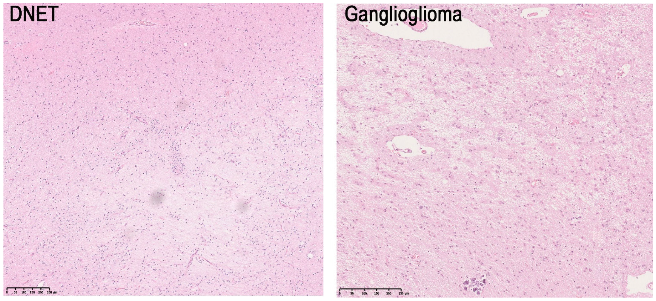
1.1. Use Case 1: Classifying Low-Grade Epilepsy-Associated Brain Tumors

Dysembryoplastic neuroepithelial tumor (DNET) and ganglioglioma (GG) are slowly growing tumors composed of both glial and neuronal cell elements and, histopathologically, are often difficult to classify [10] (see Figure 1).

They account for 1–2% of all brain tumors and do not metastasize or spread beyond the primary site of origin. These tumors occur mainly in children and young adults with long-standing drug-resistant epilepsy. The average age at seizure onset was 12 years in 984 GG and 14 years in 565 DNET when reviewing a large European cohort of 9523 patients who underwent epilepsy surgery. Seizures are commonly focal with or without secondary generalization, and neurosurgical resection has proven as the most successful treatment option. Malignant transformation has been reported for the group of GG [11,12], whereas DNET rarely show this behavior [13]. Therefore, a precise histopathological diagnosis and differentiation of these two tumor entities is important for clinical patient management [14]. The problem is that even in specialized medical centers the inter-rater agreement on the diagnosis accounts for only 40% of these tumors [10]. The DL task was to develop, therefore, a binary classifier distinguishing between the two entities.

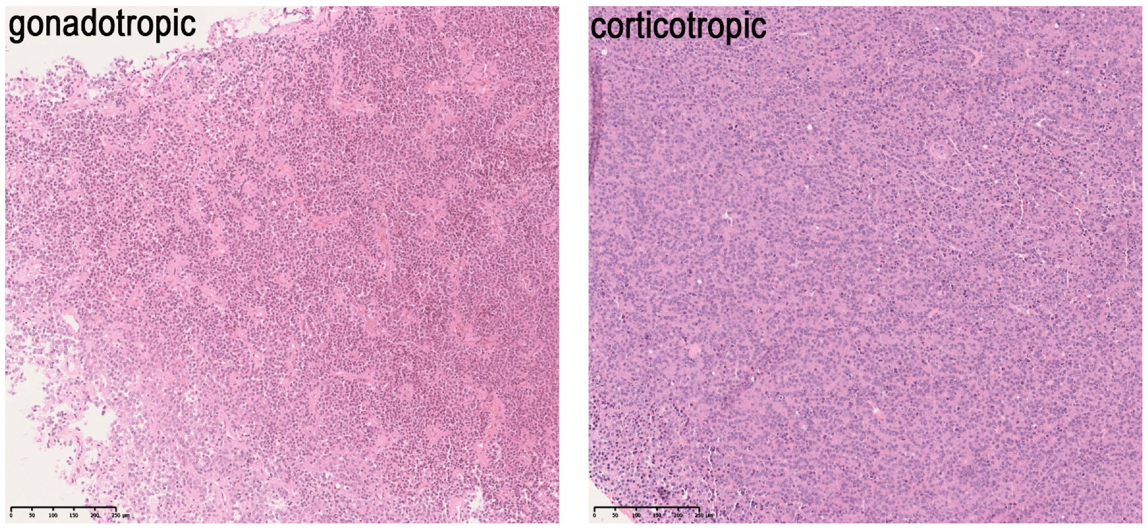
1.2. Use Case 2: Prediction of Pituitary Adenoma Subtypes and Their Neuroendocrine Features

Better neuroimaging techniques and diagnostic modalities recognize more pituitary adenomas than previously thought [15]. We consider three clinical subclasses: Pituitary adenomas with A. prominent neuroendocrine symptoms, B. slowly developing, insidious, nonspecific complaints delaying accurate diagnosis, or C. incidentally detected adenomas being symptom-free. It remains, therefore, challenging to accurately determine the prevalence and incidence of pituitary adenomas in the general population. They account for 15% of all intracranial neoplasms, being the third most frequent tumor type after meningiomas and gliomas. In multiple postmortem studies, the mean prevalence of pituitary adenomas was 14.4% [15] . The overall estimated prevalence of pituitary adenomas in the general population was calculated as 16.7%. Radiography studies showed a higher prevalence of 22.5% [15,16]. The tumor has its maximum age frequency in patients between 40 and 60 years of age. The frequency of different subtypes varies depending on the age and gender of the patients [16] .

The WHO classification of pituitary adenoma from 2017 is based mainly on the hormone and transcription factor expression of the adenoma cells [17] . In common routine workup for adenomas of the pituitary gland, the morphological evaluation is based, therefore, on H&E and a panel of immunohistochemical staining for all pituitary hormones (adrenocorticotropic hormone (ACTH), luteinizing hormone (LH), follicle-stimulating hormone (FSH), prolactin (PRL), thyroid-stimulating hormone (TSH), and somatotropic hormone (STH)) and transcription factors. In our study, we focused on corticotroph and gonadotroph adenomas (see Figure 2) since they represent the most common subtypes. We labeled our tumor samples of corticotroph and gonadotroph adenomas accordingly, e.g., corticotroph adenoma, gonadotroph adenoma with the expression of LH, and gonadotroph adenoma with the expression of FSH. As adenomas are often nonexclusively positive for only one hormone, many cases received more than one label. Therefore, we chose to tackle the problem as a multilabel approach, which means that the different classes are rated and scored individually, and possible correlations must be learned by the CNN. To make sure that the labels are correct for each tile, we manually reviewed the extracted regions from the H&E slides with the corresponding regions in the immunohistochemically stained images. In addition, we included those corticotroph adenomas as a separate class, in which the patient does not show clinical symptoms of Morbus Cushing (silent corticotropic adenoma). The DL tasks were to classify entities of adenomas of the pituitary gland from H&E-stained slides as well as to predict the clinical parameter of asymptomatic or clinically silent corticotroph adenomas.

What is new:

The depicted library enables users to perform DL with state-of-the-art techniques without the burden of managing WSI-associated overhead, such as pyramid level control or region-specific mapping, as it is kept away from the user. Additionally, the library is fully compatible with one of the most popular deep learning frameworks “fastai” which is based on “PyTorch”.

Related work:

In the context of neuropathology-related tasks, few works have been published. Some work has been completed on classifying and detecting Alzheimer‘s associated lesions, such as extracellular amyloid and intracellular tau deposits [4,18,19]. The latter approach has also been used to classify other tauopathies such as Pick’s disease for example [20]. Additionally, with the help of deep learning new disease-correlating features were identified in the white matter of different tauopathies [21]. Classifying glioma and differentiating glioma subtypes from H&E-stained slides and molecular markers was another successful task accomplished [22]. In our own recent project, we could discriminate between phenotypically very similar but genotypically different lesions of focal cortical dysplasia type IIb and tuberous sclerosis complex [3].

2. Materials and Methods

2.1. The Library

Compared to common image datasets consisting of small files in, e.g., PNG or TIFF format, WSI provide more challenges in the context of training a neural network with them. First, there is the size. A WSI’s typical size in the realm of Neuropathology is 0.5–3 Gbyte. Therefore, it is impossible to feed an entire WSI let alone a batch of WSI into a CNN, since graphic processing units or graphic cards (GPUs) do not have enough memory. So WSI need to be divided into smaller images usually referred to as tiles. WSI are also stored in special file types and most WSI scanner manufacturers provide their own. Usually, WSI are not independent of each other. A WSI belongs to a case, and a case belongs to a patient. This is important for the dataset split and evaluation of the model after the training. It is common practice to not mix data from one patient in the training, validation, and test set. For evaluation, it is interesting how the model performs on tile level, but usually, the performance on WSI, case or patient-level has a higher value in practice. So, these connections need to be tracked throughout the whole process from preprocessing until postprocessing/evaluation. Our library [23] is meant to help with this common overhead in preprocessing and the evaluation for training a classification model with WSI.

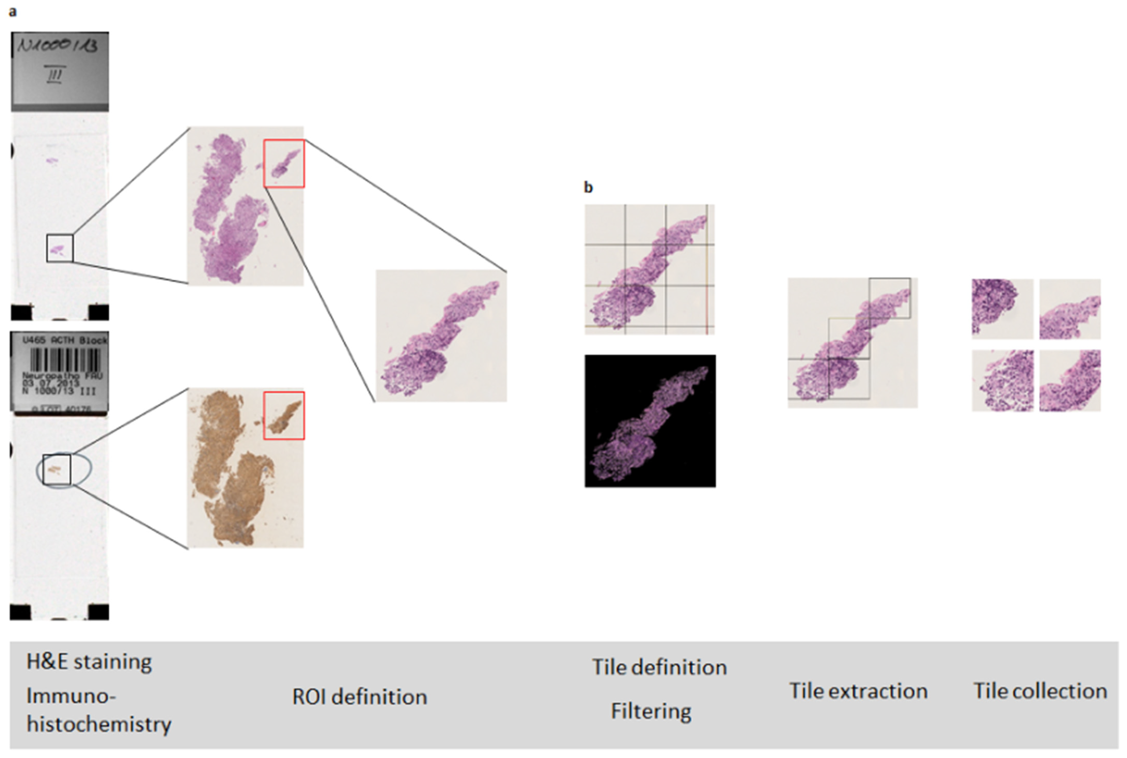
2.2. Tile Calculation

The first step is to split a WSI into multiple small tiles. A complete sample pipeline can be found in the GitHub repository of the library (https://github.com/FAU-DLM/wsi_processing_pipeline/tree/master/tile_extraction/example.ipynb, accessed on 15 December 2021) and the repositories of the two use cases (https://github.com/ChristophNeuner/DNET_vs_Ganglioglioma/blob/main/dnet_vs_gg.ipynb, accessed on 15 December 2021) (https://github.com/ChristophNeuner/glioblastoma_methylation/blob/master/methylation_status_binary_classification.ipynb, accessed on 15 December 2021).

Usually, not all parts of a WSI are of interest for further processing. So, in general, there are two main ways of making sure only the relevant parts are used: marking the interesting regions manually or using some sort of filtering algorithms that, e.g., distinguish tissue from the background, filter out pencil markings, or blurred tissue. Both ways are supported by the library and will be further explained in the following lines.

2.3. Filters Applied on Complete WSI

Our library originated as a fork of Deron Eriksson’s GitHub repository “python-wsi-preprocessing” (https://github.com/deroneriksson/python-wsi-preprocessing, accessed on 15 December 2021), which was originally written and used for his and his team’s participation in the Tumor Proliferation Assessment Challenge 2016 (TUPAC16) [24].

Most parts of this library have had a substantial rewrite, and many additions were made since. However, the filters were mostly kept untouched. Documentation about them can be found in Deron Erikson’s GitHub repository (https://github.com/deroneriksson/python-wsi-preprocessing/blob/master/docs/wsi-preprocessing-in-python/index.md#apply-filters-for-tissue-segmentation, accessed on 15 December 2021) [25] .

2.4. Calculation of Tile Locations

Our preferred way of defining the polygonal regions of interest (ROIs) in a WSI is to use the program QuPath [26] (Supplement S7). The next step is to extract the coordinates of the polygons’ vertices. We wrote a small QuPath script that can be used in the “Automate” Tab in QuPath and exports the polygons’ vertices’ coordinates into a JSON file (https://github.com/FAU-DLM/wsi_processing_pipeline/blob/master/QuPath_scripts/polygon_points_to_json.groovy, accessed on 15 December 2021).

The next step is to convert this information into RegionOfInterestPolygon objects (https://github.com/FAU-DLM/wsi_processing_pipeline/blob/master/shared/roi.py#L66, accessed on 15 December 2021). There is a convenience function if the ROIs were annotated and extracted with our script from QuPath. (https://github.com/FAU-DLM/wsi_processing_pipeline/blob/master/shared/roi.py#L195, accessed on 15 December 2021)

It is important to notice that this part is completely optional. The ROI definition may be skipped.

Subsequently, all relevant tile locations are calculated. For this process, the function “WsisToTilesParallel” (https://github.com/FAU-DLM/wsi_processing_pipeline/blob/8c5e4a360fa369221ce86dd35837e91f31817d30/tile_extraction/tiles.py#L1275, accessed on 15 December 2021) is used. It calls the function “WsiToTiles” for every WSI and runs in parallel. It takes a few interesting parameters. We will elaborate on a few here; the rest is covered in the function’s docstring.

“wsi_paths”:

First of all, a list with the paths to the WSI files has to be passed. Notice that not only WSI files but also PNG files are supported. If one has already extracted the interesting parts of the WSI as PNGs, one can use them without specifying ROI coordinates, as described before.

“grids_per_roi”, “optimize_grid_angles”, “angle_stepsize”, “minimal_tile_roi_intersection_ratio”:

The library lays a grid of all possible tiles over each ROI (Supplement S8). If no ROI is specified, the library internally creates one ROI, which simply spans the complete WSI.

The logic for this part of the pipeline resides in the tiles.py module, to be more specific, in the Vertex, Rectangle, Grid, and GridManager classes. A Vertex object represents one vertex of the polygonal ROI and provides simple arithmetic operations such as add, subtract, and multiply with scalars and matrices. It also provides the functionality to rotate itself around a specified point. This is performed by multiplying a rotation matrix with the vertex coordinates represented as a 2×1 vector.

$$\mathrm{Rotation} \mathrm{Matrix}\begin{array}{c}x\prime \\ y\prime \end{array}=\left[\begin{array}{cc}cos\left(\alpha \right)& -sin\left(\alpha \right)\\ sin\left(\alpha \right)& cos\left(\alpha \right)\end{array}\right]\left[\begin{array}{c}x\\ y\end{array}\right]$$

The Vertex class also provides a convenience function to change the WSI level of the coordinates. Because of its size, a WSI is stored in a pyramid-like format (Supplement S10) in multiple images per level. So particular regions of the image are loaded on-demand with higher resolution while zooming in. Therefore during the process of tile calculations, it is important to specify the zoom level for a given coordinate. So, it is often necessary to convert various coordinate values to another zoom level. All the filtering steps for example in our pipeline are performed on a scaled-down version by the factor 32 of the WSI to enhance the speed and obtain the results in a reasonable time.

A Rectangle object represents the bounds of a tile. It also wraps necessary functionality, such as rotation. The Grid class implements all the functionality to represent a grid of Rectangles and, therefore, possible tile locations that are laid over a ROI. Finally, there is the GridManager class. It creates as many Grid objects for each ROI as is specified in “grids_per_roi” and contains some convenience functions for, e.g., visualization. It also merges overlapping ROIs. The full spectrum of the functionality of these classes can be seen on GitHub: https://github.com/FAU-DLM/wsi_processing_pipeline/blob/master/tile_extraction/tiles.py#L78, accessed on 15 December 2021.

If “grids_per_roi” is greater than one, multiple slightly shifted grids are laid over each ROI. This increases the number of tiles and therefore the amount of training data. This means that the same tissue is present in multiple tiles but, nonetheless, all tiles are unique. If “optimize_grid_angles” is true, the grid is rotated in an iterative approach by “angle_stepsize” in each iteration, and the angle, which results in the most tiles per ROI, will be used for further calculations. This is completed for each ROI individually. So the smaller the “angle_stepsize” is, the closer the angle gets to the optimum, but the longer the process takes. The last important parameter in this context is “minimal_tile_roi_intersection_ratio”. If it is 1.0, only tiles that lay 100% in the ROI will be considered for further processing. The closer it gets to 0.0, the more tiles can be outside of the ROI, but never completely, since 0.0 is outside of the possible range of this value.

2.5. Tile Filtering

Among these tiles, there might still be some, which are not worth keeping. If ROIs are specified, this amount should be fairly small, but if no ROIs are specified, there should be plenty to be filtered out. The user of the library can specify a tile scoring function that only takes the tile in form of a PIL image as a parameter and returns a score for it. The user also has to provide a threshold for that score. All tiles with a score above this threshold pass filtering and will be considered for training.

The library provides a default tile scoring functionality that works for H&E-stained slides.

$$score=1-\frac{10}{10+\frac{tissuePercentage\ast colorFactor\ast saturationAndValueFactor}{1000}}$$

The scoring formula generates good results for the images in the dataset and was developed through experimentation with the training dataset.

The first criterion is the amount of tissue in a tile. To separate tissue from the background we applied four filters to a tile image (Supplement S9). First, the image was converted to greyscale; then, its complement was created. After that Otsu’s threshold was applied. Thresholding using Otsu’s method is a popular thresholding technique. This technique was used in the image processing described in A Unified Framework for Tumor Proliferation Score Prediction in Breast Histopathology [27].

The colorFactor value is used to weigh hematoxylin staining heavier than eosin staining. Utilizing the Hue-Saturation-Value (HSV) color model, broad saturation and value distributions are given more weight by the saturationAndValueFactor. The score is scaled to a value from 0.0 to 1.0.

Tissue with hematoxylin staining is most likely preferable to eosin staining. Hematoxylin stains acidic structures such as DNA and RNA with a purple tone, while eosin stains basic structures such as cytoplasm proteins with a pink tone.

Differentiating purplish shades from pinkish shades can be difficult using the RGB color space [28]. Therefore, to compute the colorFactor value, we first convert the tile’s RGB color space to an HSV color space [29]. In this color model, the hue is represented as a degree value on a circle. Purple has a hue of 270 degrees and pink has a hue of 330 degrees. We remove all hues less than 260 and greater than 340. Next, we compute the deviation from purple (270) and the deviation from pink (330). We compute an average factor which is the squared difference of 340 and the hue average. Saturation and value standard deviations should be relatively broad if the tile contains significant tissue. The colorFactor is computed as the pink deviation times the average factor divided by the purple deviation. It favors purple (hematoxylin stained) tissue over pink (eosin stained) tissue. The information about one tile is then stored in a Tile object.

The result of the filtering process is a TileSummary object for each WSI. A TileSummary object contains the information about the WSI including dimensions, scaled dimensions, which were used for faster tile calculations, ROIs, the GridManager object, and all tiles. It also implements some visualization methods to display the WSI with ROI and tile boundaries.

In the next step, the PatientManager class in the wsi_processing_pipeline.shared.patient_manager.py is important. Its main purpose is to manage the hierarchical structure of a pathological dataset. A tile belongs to an ROI. An ROI belongs to a WSI. A WSI belongs to a case, and a case belongs to a patient. It is good practice to split datasets on the patient level. To measure the performance of a model after training, not only can model performance on a tile level be evaluated, but also performance on the WSI or case level is easily assessable. Therefore these relationships are conserved by the PatientManager. It is also responsible for setting the labels of each tile. The PatientManager class additionally implements some convenience functions for dataset splitting into a training, validation, and test set and for a k-fold cross validation split. It can print out a class distribution and is capable of undersampling the dataset.

In the next step, the fastai [30] library takes over for training the neural network. During tile filtering, the user of our library can specify in the WsiToTiles function if each tile should be extracted and stored to disc as a PNG file. We wrote a custom fastai ImageBlock called TileImageBlock that works with fastai’s data block API. This allows renouncing saving each tile to disc because the TileImageBlock can extract a tile image on the fly during the training process given the spatial information about a tile that is stored in each Tile object. This has the advantage of consuming less storage space and since it is usually necessary to play around with the parameters that are used for filtering until only the desired tiles are left, not saving the tiles is a huge speedup for this part of the process.

Our preferred library for training a neural network is fastai [30], which is built on top of Facebook’s increasingly popular PyTorch [31] library.

After training has finished, evaluating the performance of the model on the validation or an unseen test set is crucial. For this use-case, we implemented the Predictor class, which resides in wsi_processing_pipeline.postprocessing.predictor.py. It takes a fastai [30] Learner and one of our library’s PatientManager class objects. In a first step, it calculates predictions for each tile image in the desired dataset. In a second step, it calculates the predictions for each WSI or case by calculating the mean raw prediction for all classes for each tile and applying a threshold that can be specified for each class by the user of the library.

The last step is to evaluate the performance of the model. We, therefore, implemented the Evaluator class in wsi_processing_pipeline.postprocessing.evaluator.py.

Its constructor takes an instance of the abovementioned Predictor class as the only argument. It implements a few commonly used methods to measure model performance. It can calculate the per-class accuracy and plot receiver operating characteristic (ROC) curves, precision-recall curves, confusion matrices (Figure 3), and probability histograms (Figure 4). It can also print out sklearn’s classification report and print a list of tiles with the highest losses or a list of cases, WSI, or tiles sorted by a user-specified metric calculated with the predictions. It is also capable of creating Gradient-weighted Class Activation Mappings (Grad-CAMs) [32].

2.6. Dataset Preparation for Both Use-Cases

Histopathology slides from all patients of interest for the study design were retrieved from the archives of the Dept. of Neuropathology (see below) and subsequently digitized using a Hamamatsu S60 scanner with a 40× magnification. We included only H&E stainings, thus, eliminating the need for more complex and expensive immunostainings. The WSI of our dataset were reviewed by two expert neuropathologists of our institute.

Use case 1: For the DNET and ganglioglioma, classifier slides from 219 patients were used. In total, 52 of them were DNETs and 167 were ganglioglioma. QuPAth was used by two of our expert neuropathologists in epilepsy pathology to define polygonal ROIs containing tumor tissue in the WSI, and we exported their coordinates to JSON files. These JSON files were then used by the library to extract tiles from the relevant regions of the WSI. In total 171,514 tiles from GG and 34,520 tiles from DNETs with a size of 1024 × 1024 pixels were defined for further processing and training.

Use case 2: To train and evaluate the pituitary adenoma classifier, H&E and immunohistochemically stained (ACTH, LH, FSH) tissue slides of 410 patients were collected. In total, 181 of these were diagnosed with corticotroph and 229 with gonadotroph adenoma of the pituitary gland (Supplement S1 and S2). Overall, the dataset consisted of 431 H&E (202 corticotroph and 229 gonadotroph) slides with the corresponding ACTH LH/FSH whole-slide images for comparing and identifying the correct ROI (Figure 5). The ROIs on an individual H&E slide were defined as regions, where the immunostainings showed tumor expressions of the specific hormone. Care was taken that no normal pituitary gland tissue was included (Figure 5). This time-consuming ROI selection process was necessary to ensure the correct labeling of each tile and, therefore, the validity of the resulting models. Otherwise, biases through wrong labeled areas could have worsened the performance. For example, areas with only connective tissue were excluded. Moreover, the hormone expression of the adenoma is not homogeneously spread over the sample. This was particularly important to consider for gonadotropic adenomas. When an adenoma expresses LH and FSH that does not mean that all subregions express both hormones. So, there can be tiles that are only labeled with LH or FSH, although the whole tumor expresses both. ROIs were defined at 40× magnification level and cropped into smaller tiles of 1024 × 1024 pixels to further preprocess and feed into our model (Figure 5). The tile extraction resulted in 206,517 gonadotropic and 63,893 corticotropic tiles.

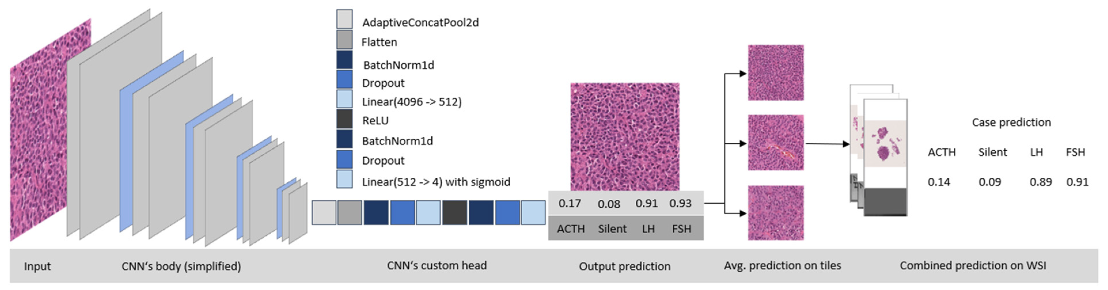
2.7. Convolutional Neural Network Architecture

Use case 1: For the DNET-GG classifier, a ResNet50 was implemented, using the open-source Python library fastai [30], which is based on PyTorch [31]. It was pretrained on ImageNet [33,34], and the classification head was replaced to predict two (DNET or GG) instead of the 1000 classes included in the ImageNet dataset (Supplement S3). In our experience, ResNet50 is often a good starting point, since it is relatively fast to train compared to more complex models with more parameters but nonetheless delivers promising results. Since it performed well on the defined dataset, it was not necessary in our view to try out another model.

Use case 2: For the pituitary gland classifier a ResNeXt-101-32x8d CNN architecture also pretrained on ImageNet [33,34] was implemented. ResNeXt-101-32x8d [35,36] was chosen, as it yielded the best results with the least overfitting out of a couple of state-of-the-art network architectures including ResNet50, se_ResNeXt101_32x4d, xception, and inceptionv4 (Supplement S5). The basic network architecture was not changed. Only a customized classification head (Figure 6, Supplement S3) was used to predict four instead of the 1000 ImageNet classes. It consisted of several pooling, batch normalization, dropout, and fully connected layers with four final output channels with a sigmoid-activation function with a threshold of 0.5 to produce individual output probabilities representing the four classes of corticotropic adenoma, silent corticotropic adenoma, gonadotropic adenoma with the expression of LH, and gonadotropic adenoma with the expression of FSH (Figure 6).

2.8. Preprocessing and Data Augmentation

Image preprocessing is an important step in every computer vision task to augment the number of samples, to prevent overfitting, and to support the model against invariant aspects that are not correlated with the label [37,38]. First, the tiles were resized to 512 × 512 pixel images to increase the possible batch size. Following this approach, we made sure to have a wider field of view per tile instead of the maximum possible resolution. In our approach, we used a pipeline of several augmentation techniques performed batch-wise on the GPU consisting of a random crop with reflection padding, randomly flipping (horizontal or vertical), and rotating by a multiple of 90 degrees, a random symmetric warp with a magnitude between −0.2 and 0.2, a random rotation between −10 and +10 degrees, a random zoom with a zoom factor between 1.0 and 1.1, and a random change in brightness with a factor between 0.4 and 0.6, where a factor of 0 will transform the image to black, a factor of 1 will transform the image to white, and a factor of 0.5 doesn’t adjust the brightness. Furthermore, an augmentation on the contrast of the image was applied with a factor between 0.8 and 1.25, where a factor of 0 will transform the image to grey, a factor over 1 will transform the picture to super-contrast, and a factor = 1 does not adjust the contrast. These augmented images were then normalized. The augmentations were applied on the fly with a randomness factor for reproducibility for every batch so that there was no need to save augmented images and one image could be augmented in multiple ways. This whole approach ensures that out of one image multiple new images of the same class can be obtained by multiplying the number of images available for training the neural network. We tried to apply as little data augmentation as possible to avoid changing special characteristics of the tissue.

2.9. Training and Evaluation

The training was performed with 16-bit precision floating-point numbers [39] using the Adam-Optimizer [40], and the initial learning rate was determined by using fastai’s learning rate finder (Supplement S4). The learning rate was adjusted during the training according to the one-cycle policy [41]. The batch size was twelve for the pituitary adenoma classifier and 35 for the DNET-GG classifier. At first, only the randomly initialized custom head (Figure 6, Supplement S3) was trained for five epochs with a maximum learning rate of 10⁻³ (Supplement S4) in both projects to not interfere with the pretrained weights of the CNN’s body. Thereafter the body’s layers were unfrozen, and the complete network was trained for ten epochs with differential learning rates between 10⁻⁹ and 10⁻⁶ for the pituitary gland adenoma classifier and between 10⁻⁸ and 10⁻⁶ for the DNET-GG classifier (Supplement S4) where earlier layers were trained with a lower learning rate than the later ones. The idea behind this is to maintain the basic image-classification patterns of the pretrained model and prevent overfitting. Training performance was controlled using accuracy with a threshold of 0.5 as a metric per tile, and the used loss function was binary cross-entropy loss. Model parameters were saved every epoch and the weights of the epoch with the best results were used for evaluation. We further evaluated model performance with five-fold cross-validation, without having any training- and validation-slide and patient overlap. After the training, predictions on the five validation sets were calculated with the corresponding model based on the combined predictions of all tiles of a case. The prediction for a case was calculated using majority voting for the pituitary gland adenoma classifier and the arithmetic mean of the raw predictions (between 0.0 and 1.0) of all the case’s tiles for the DNET-GG classifier. These results were then combined and used to calculate true and false-positive rates, which were then used to plot Receiver Operating Characteristic curves, true/false positive frequency histograms, and in conjunction with false-negative rates to plot precision-recall curves.

Since silent corticotroph adenomas only made up 9.7% of the dataset, we decided to train a second neural net on an undersampled training set. The original training set (80% of the complete dataset) consisted of 226,422 tiles of which 59% were positive for LH, 62% for FSH, 22% for ACTH, and 9.4 % were silent corticotroph adenomas. After the undersampling procedure, 54,713 tiles were left of which 43% were positive for LH, 43% for FSH, 43% for ACTH, and 39 % were silent corticotroph adenomas. We assured that at least 30 tiles per WSI were left after undersampling. Again, we used the resnext101_32x8d architecture. The head was trained for five epochs with a maximum learning rate of 10⁻³. The complete model was then trained for ten epochs with maximum discriminative learning rates ranging from 10⁻⁷ to 10⁻⁵. In both cases, the one-cycle learning rate policy was used with minimum learning rates of 1/25 of the maximum learning rates.

2.10. Hardware

We implemented our approach on a local server running Ubuntu (18.04 LTS) with one NVIDIA GeForce GTX 1080Ti and one NVIDIA Titan XP, AMD CPU (AMD Ryzen Threadripper 1950X 16 × 3.40 GHz), 128 Gb RAM, CUDA 10.2, and cuDNN 7.

2.11. Availability and Implementation

The datasets generated and analyzed during the presented study are not publicly available, but parts of the pipeline used in this project including training and visualization are available on our Project Homepage.

https://github.com/FAU-DLM/wsi_processing_pipeline, accessed on 15 December 2021.

https://github.com/ChristophNeuner/pituitary_gland_adenomas, accessed on 15 December 2021.

https://github.com/ChristophNeuner/DNET_vs_Ganglioglioma, accessed on 15 December 2021.

3. Results

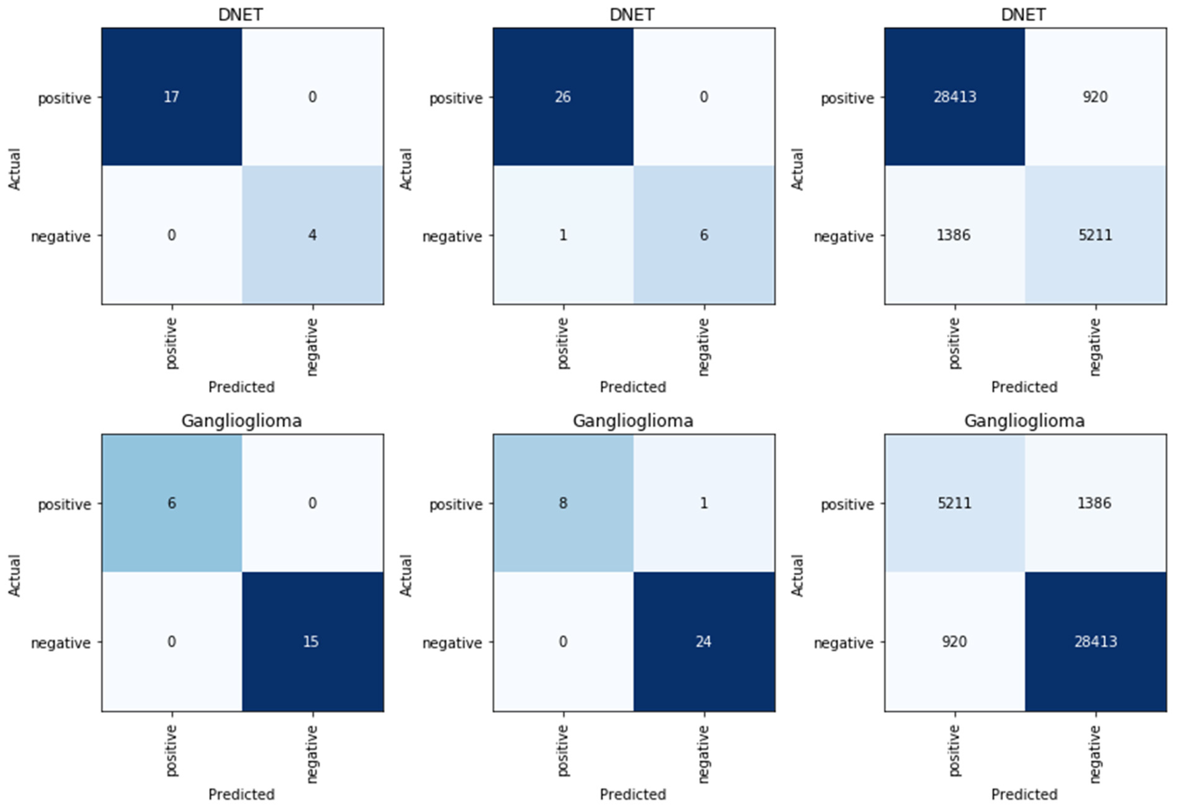
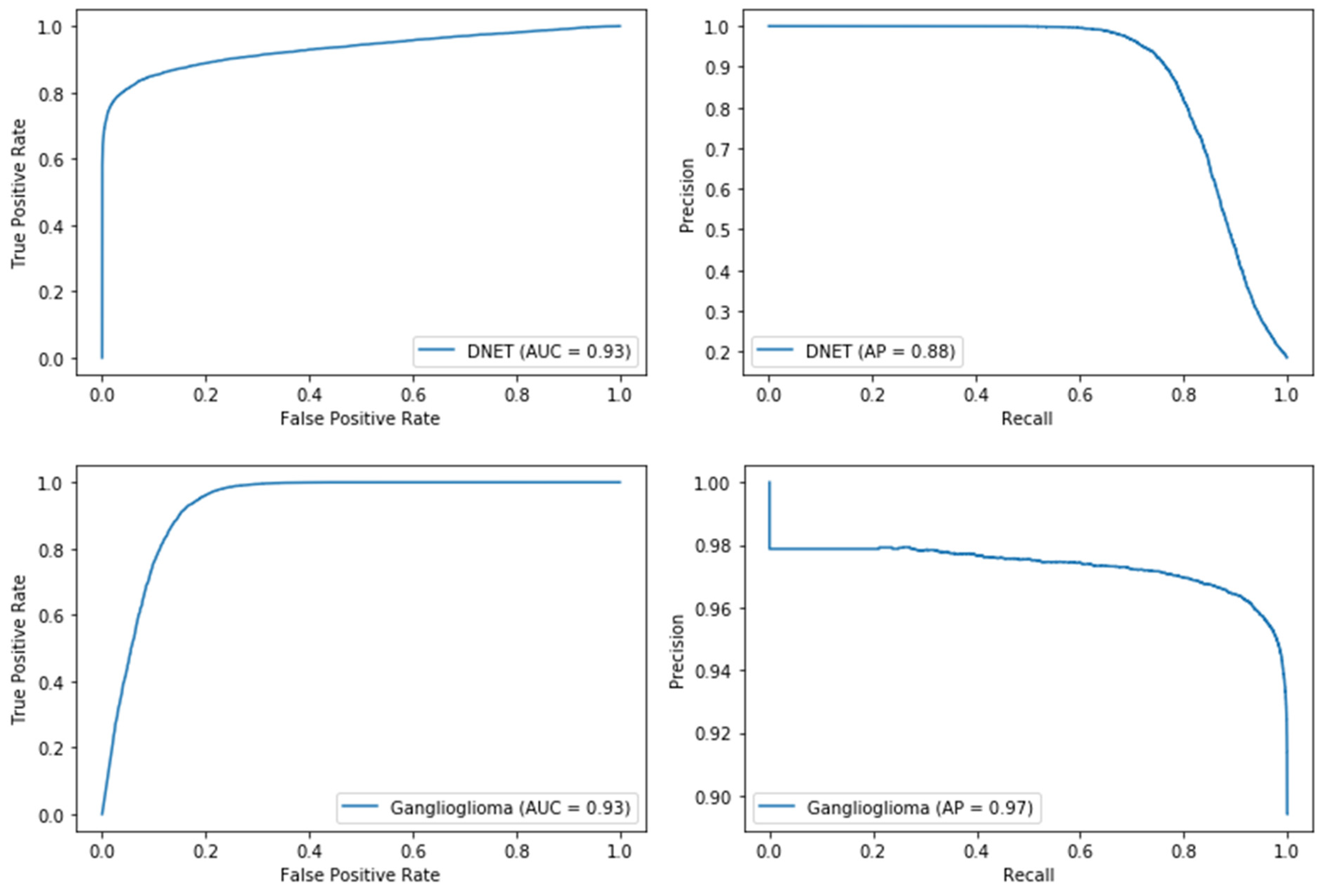
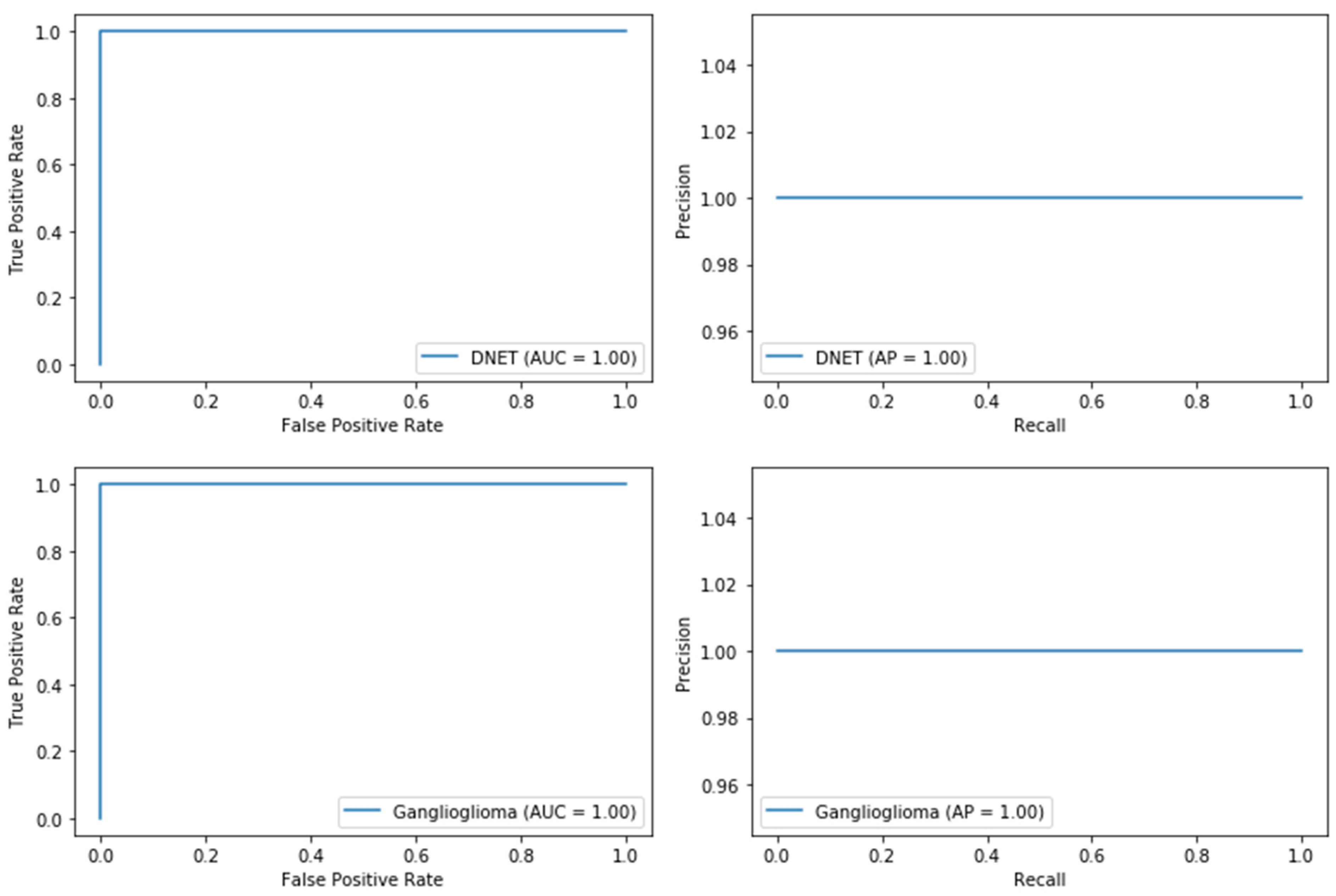
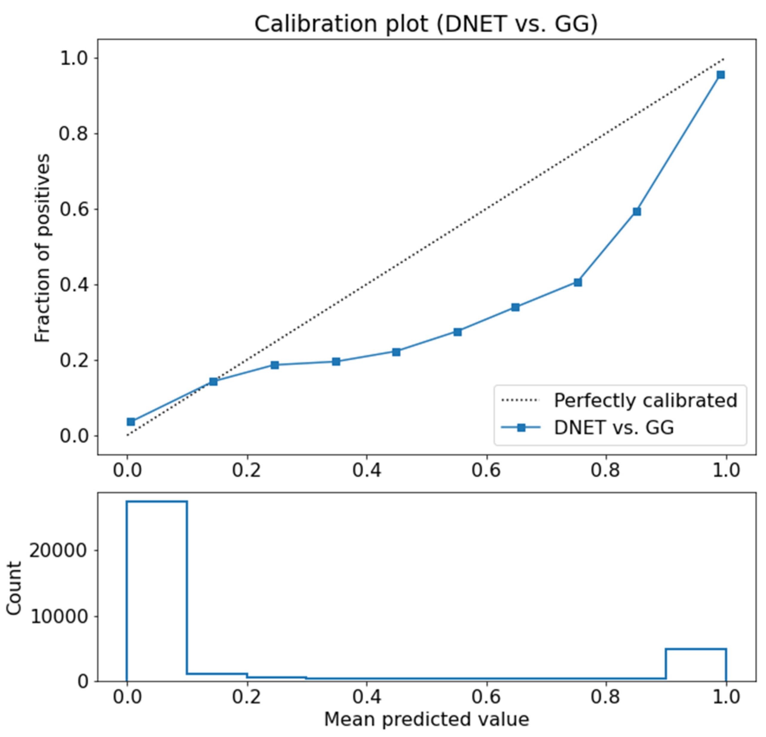
3.1. Use Case 1: DNET-GG Classifier

We evaluated the performance on the validation set, which made up 20% of the whole dataset and was not used for training. It consisted of 24 slides of ganglioglioma and seven slides of DNET. In total, 29,333 tiles were extracted from the GG slides and 6597 tiles were extracted from the DNET slides for evaluation. No hyperparameter tweaking was performed, which could have led to overfitting on the validation set. On a tile level, the accuracy was 0.936 and on a slide level 0.968. The Brier score on the tile level was 0.053 and 0.022 on the slide level. The AUC on the tile level was 0.93 and 1.00 on the slide level for the ROC curve. The average precision calculated from precision and recall was 0.88 for DNET and 0.97 for GG on the tile level. On the slide level, it was 1.00 for DNET and GG. (Figure 7 and Figure 8)

Model calibration was also evaluated on tile level (Figure 9). We observed tiles that were overconfidently classified by the model as DNET but were in fact GG. DNETs typically contain mucus and have a loosened-up structure. Tiles from GGs which were wrongly classified as DNETs also had a loosened-up structure, which was only artificial.

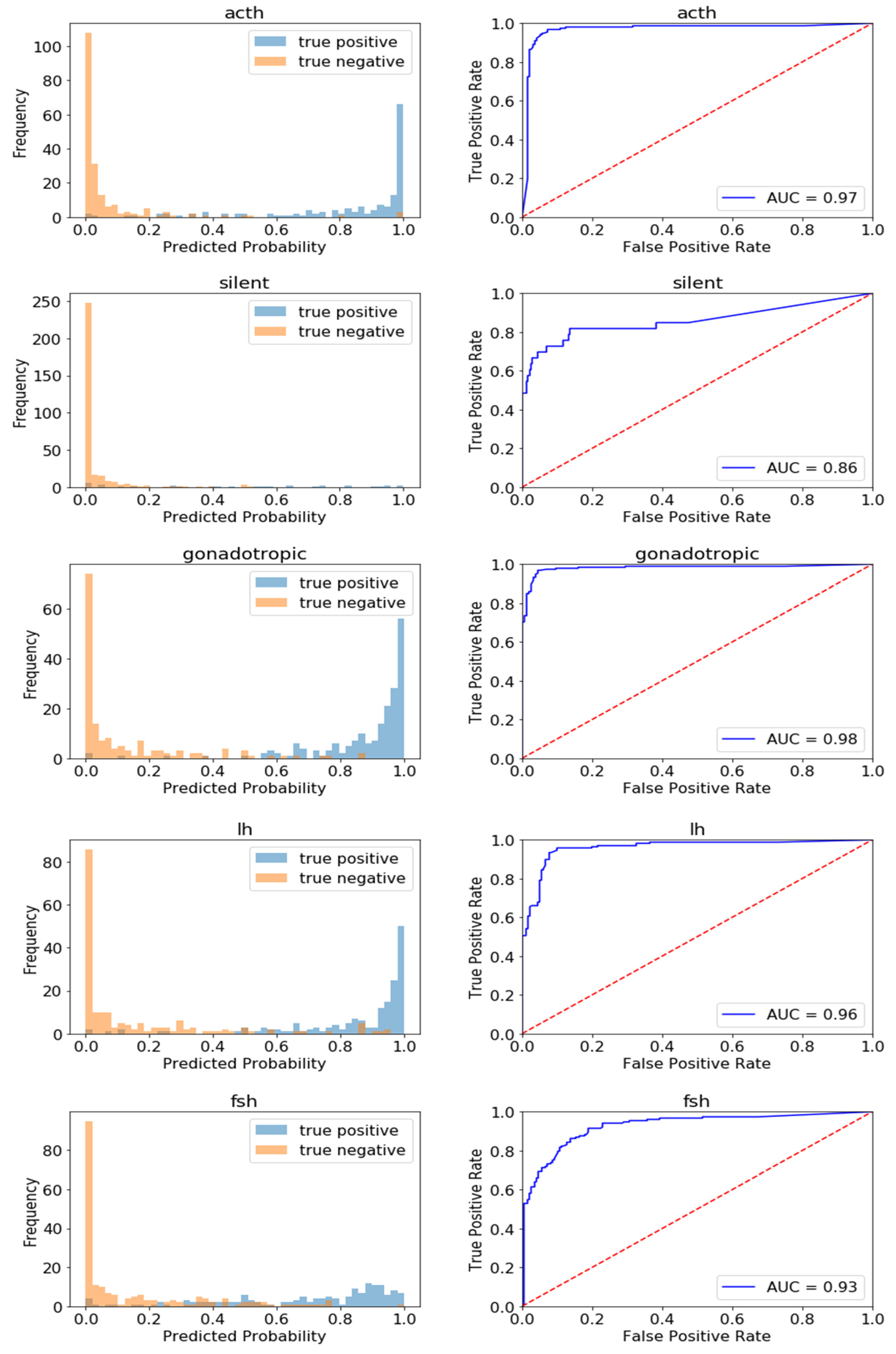
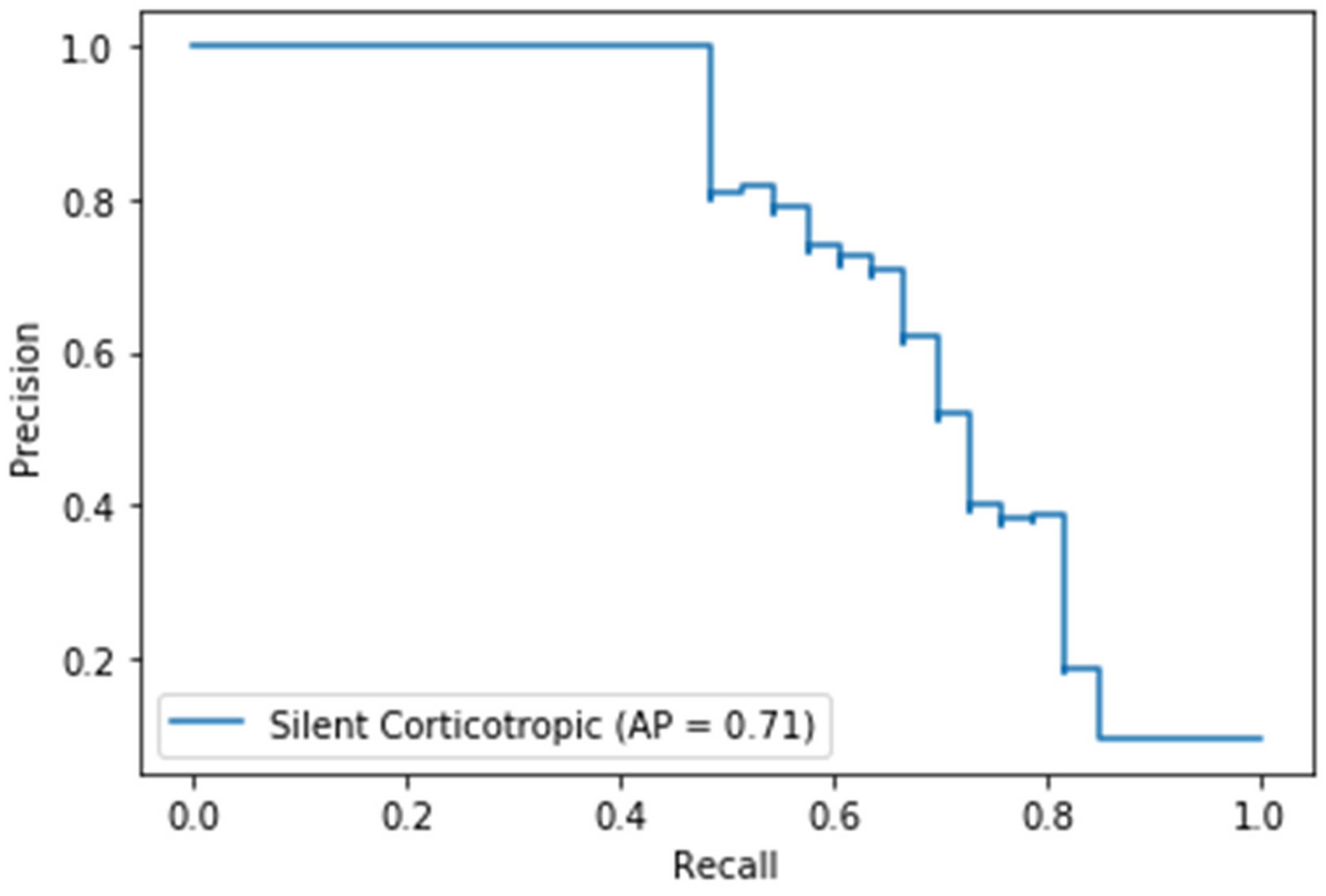
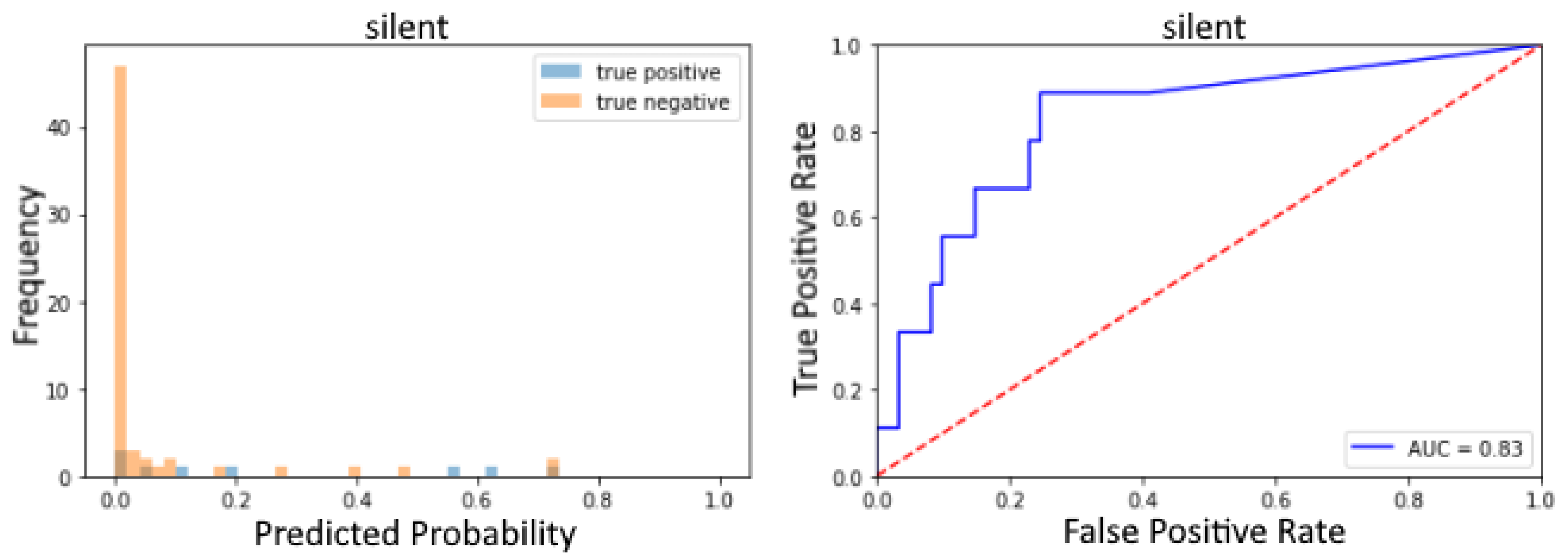
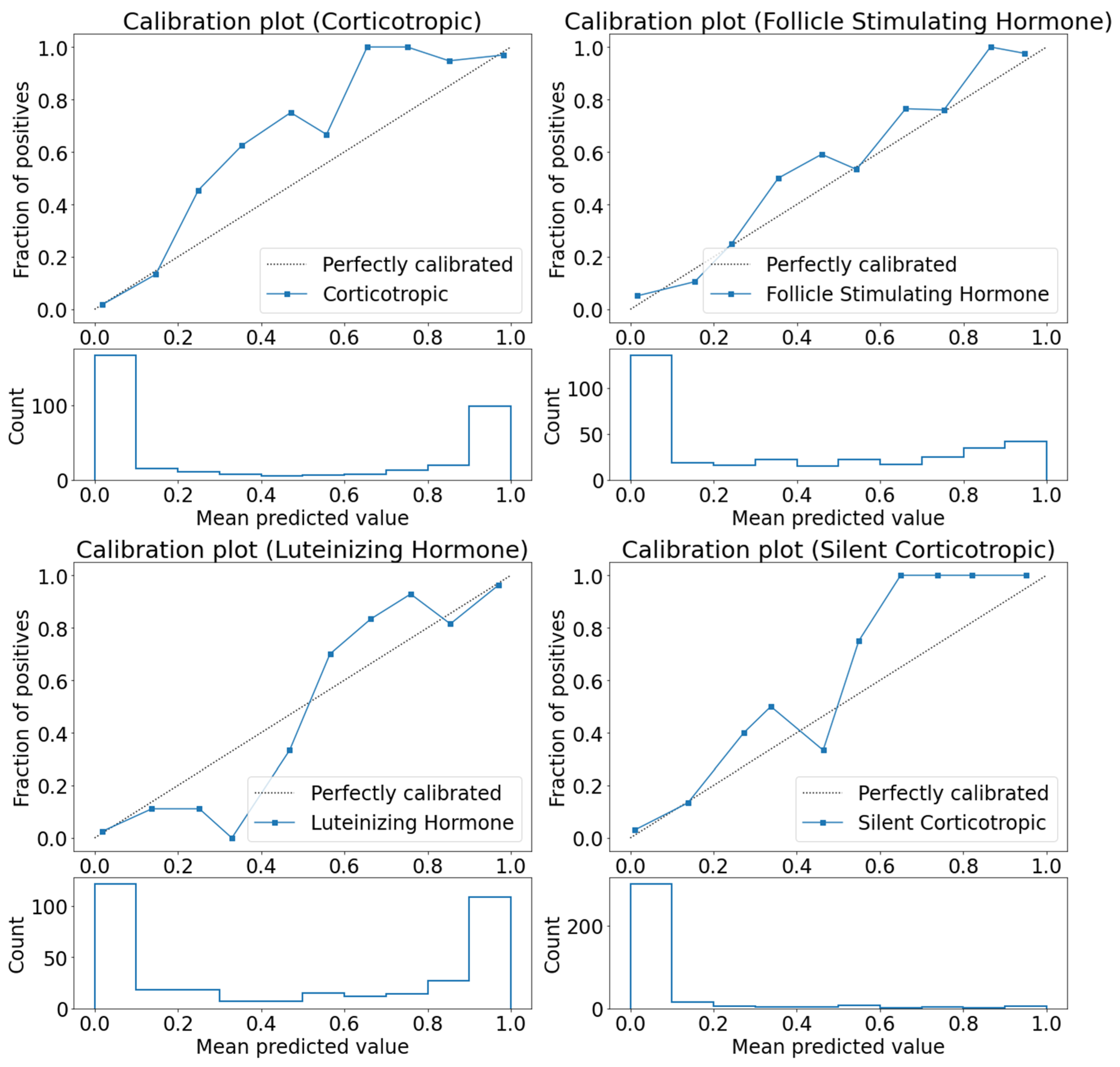
3.2. Use Case 2: Pituitary Adenoma Classifier

All CNN were trained to classify the ROIs containing adenoma and surrounding tissue. First, we performed a study to determine which model to use for our classification task. We tested ResNet50, ResNet101, ResNet152, DenseNet121, Xception, Inceptionv4, se_ResNext101_32x4d and ResNext101_32x8d. We compared those models on a predefined validation set with accuracy calculated on a case basis for each class with a threshold of 0.5 (Supplement S5). Inceptionv4, se_ResNext101_32x4d and ResNext101_32x8d showed similar promising results. We decided upon ResNext101_32x8d because of the slightly better test-set results. During training validation, accuracies mostly stayed above training accuracies, and validation loss stayed below training loss values, indicating little to no overfitting on the training dataset. We finally evaluated our model via five-fold cross-validation. For each model within the process of cross-validation, we took 80% of the dataset as training data and 20% as validation data. There was no overlap between these five validation sets. All five validation sets showed similar AUCs with no significant outliers (Supplement S6). Then predictions were made for all tiles of the five validation sets with the respectively corresponding model that was not trained on that particular validation set. Via majority voting with a threshold of 0.5, we then calculated the labels on a case basis and computed AUCs of ROC curves for each class. If more than 50% of the tiles of one case were labeled with the class ACTH, the whole case received the label ACTH.

For ACTH the Brier score was 0.054, for silent ACTH 0.046, for LH 0.069, and for FSH 0.10.

For ACTH the AUC of the ROC curve was 0.97 with a proportion of 44.7% of all cases. The AUC for silent ACTH was 0.86 with a proportion of 9.7%. The AUC for gonadotropic (LH and/or FSH) was 0.98 with a proportion of 55.3%. The AUCs of LH and FSH alone were 0.96 and 0.93 with proportions of 48.1% and 43.8% (Figure 4). Since the silent ACTH cases only made up 9.7% of the dataset, the AUC of 86% of the ROC curve could have simply been a result of guessing. Therefore, we also calculated a precision-recall curve (Figure 10), which resulted in an AUC of 0.71, and, furthermore, trained another neural net on an undersampled dataset as described in the last paragraph of “Training and Evaluation”. We reached an accuracy of 88.6% and an AUC of 0.83 for the ROC curve on the validation set for the silent ACTH class (Figure 11).

We also evaluated the calibration state of our model for the four different classes on slide level (Figure 12). We identified WSI for which the model’s prediction differed the most from the true label. Tile quantity and tissue quality had the most influence on the quality of the prediction. If there was only little amount of adenoma present and this tissue was infused with non-pituitary cells, such as blood, connective tissue, or bone, the model had problems predicting the correct class.

4. Discussion

We developed a whole slide image processing library [23] addressing the needs of researchers to assess different DL tasks without the hurdles of complex dataset management. The large size of WSI and annotation of multiple regions of interest tend to increase such technical obstacles. It is also desirable to extract all tiles on the fly during training and only save their spatial information but not the images. This pipeline has the advantage of being more flexible. It is not necessary anymore to repeatedly store extracted tiles as images to disc, saving space and time. Moreover, the evaluation of the trained model requires more steps when dealing with WSI. Results on the tile level are only of limited significance. They have to be transformed into predictions for the complete WSI and the entire case. For histopathologists or expert clinicians addressing a clinical hypothesis, these hurdles may become a real burden. Further, DL experts familiar with the usage of DL frameworks may underestimate the specific handling of digital pathology-associated tasks. The new library provides convenient ways of dealing with WSI in the realm of Neuropathology, thereby facilitating access to DL for both groups of researchers.

Access from and to different levels of magnification, region of interest definition, and handling, as well as dataset splitting, are essential mechanisms and tend to be technically intricate. The library manages these crucial steps and offers default parameters enabling the user to focus on the problem-specific tasks. For the specific use-cases addressed in this study, the library facilitated the management of pre-extracted image patches for a given patient as well as extraction of image patches on the fly from predefined ROI. Our evaluation of different state-of-the-art model architectures to identify the most suitable model for the problem-specific tasks, i.e., best classification results and least overfitting, resulted in the selection of resnet50 for the first use-case and the resnext101_32x8d [35,37] architecture for the second use-case. We believe that these rather large networks with lots of parameters worked well, because of their large input image size of 512 × 512 pixels. On smaller images, networks with fewer parameters tend to work better in our experience [3]. A crucial step in our pipeline was the way of image preprocessing. One part of this aspect was image augmentation to increase the variance presented to the network [42]. Normalization of the input data was performed with the mean and standard deviation of our own dataset. Fastai [30] does this conveniently for the user.

Use-case 1: In the first use-case, we developed a DL approach to distinguish between two epilepsy-associated tumors, the GG and the DNET. Since unlike DNET, some GG can undergo malignant transformation [11,12], a precise distinction between these two entities is crucial. We were able to demonstrate that a CNN can differentiate between these two entities with a very high accuracy only using H&E-stained slides. This confirms the potential of DL in assisting pathologists in their decision-making diagnostic process and to eventually reducing the necessity for further stains.

Use-case 2: In the second use-case addressed, we developed a DL approach to help to diagnose the entity of pituitary adenomas without the necessity of additional immunohistochemical stainings. Additionally, we could show that even a clinical parameter, such as the clinical occurrence of M. Cushing of corticotroph adenomas, might be hidden within the tissue; however, it could successfully be recognized by our neural network approach. This evidence supports the hypothesis that clinical parameters can be found within histomorphology, and that distinct features may be revealed by DL in terms of imaging biomarkers. Guided Grad-CAMs [32] could now be used to visualize the decision making and to teach pathologists which morphological structures are crucial for the network in its decision-making process.

We addressed the classification task on predictions per tile and collected all votes for the given slides of a patient’s case. We then obtained the final diagnosis by majority voting to obtain predictions on a case basis. If more than 50% of the tiles of one case were labeled with one class, the case was given that class label. We chose that option for two reasons.

First, different from finding metastasis in lymph nodes where high sensitivity is needed, histological slides from pituitary adenomas usually contain massive adenoma; hence, most of the tissue on the slide belongs to the tumor. Second, time was not a major concern. We could simply take and analyze all possible tiles instead of only taking a representative batch for inference.

Limitations and Potential Solutions Moving into the Future

A well-recognized obstacle in digital pathology represents batch effects including variation in staining intensity or fixation artifacts [4,43]. We contained such batch effects in our input data through hand-picked ROI and normalization. We did not directly address the problem of stain normalization [44]for this dataset, because all staining was performed in a single lab, and only one device was used for scanning. For further usage of our model in a production environment with whole slide images from other institutes, this would be crucial. We are continuously working on this issue to make our models more robust in the future.

Histopathology analysis represents a gold standard in tumor diagnosis as it often directs further treatment. Adenomas of the pituitary gland, although routinely classified by immunohistochemical profiling of their neuroendocrine axis, are in urgent need of a clinically meaningful histopathology classification of their risk for relapse. This was partially addressed by the WHO classification from 2004 and 2016. The criteria of atypia to label more aggressive adenomas has been removed, however, as it has not proved a predictive marker [17,45]. The “silent” corticotroph class of our dataset did represent another clinical parameter of interest and was remarkably well recognized by our network, even in the evenly distributed dataset. The good classification result of the “silent” corticotroph class in our study shows that neuronal networks are capable of revealing such clinical information hidden within tissue slides and, hence, it may also be possible to extract a clinical relapse parameter from tissue slides via DL. However, due to the lack of datasets stained at different labs, digitized from different scanners, and the size of the dataset, our well-performing models may be unsuitable for clinical practice yet.

In conclusion, we developed a convenient open-access library compatible with fastai to support hypothesis-driven DL research projects in the realm of neuropathology.

It helps in managing the dataset by assigning hierarchy levels such as patients, cases, and slides, thereby making it easily possible to split the dataset for training and evaluation. The library consists of building blocks fully compatible with fastai for easy integration and usage of the full spectrum of fastai functionality. Additionally, many visualization methods for evaluation are implemented.

Both use-cases demonstrated the successful diagnosis of adenoma of the pituitary gland and distinguishing between DNET and GG by H&E-stained slides only and without the necessity of cost- and labor-intense immunohistochemistry staining.

References

1. Bejnordi, B.E.; Veta, M.; Van Diest, P.J.; Van Ginneken, B.; Karssemeijer, N.; Litjens, G.; Van Der Laak, J.A.W.M.; Hermsen, M.; Manson, Q.F.; Balkenhol, M.; et al. Diagnostic Assessment of Deep Learning Algorithms for Detection of Lymph Node Metastases in Women With Breast Cancer. JAMA 2017, 318, 2199–2210. [Google Scholar] [CrossRef]
2. Arvaniti, E.; Fricker, K.S.; Moret, M.; Rupp, N.; Hermanns, T.; Fankhauser, C.; Wey, N.; Wild, P.J.; Rüschoff, J.H.; Claassen, M. Automated Gleason grading of prostate cancer tissue microarrays via deep learning. Sci. Rep. 2018, 8, 12054. [Google Scholar] [CrossRef]
3. Kubach, J.; Muhlebner-Fahrngruber, A.; Soylemezoglu, F.; Miyata, H.; Niehusmann, P.; Honavar, M.; Rogerio, F.; Kim, S.H.; Aronica, E.; Garbelli, R.; et al. Same same but different: A Web-based deep learning application revealed classifying features for the histopathologic distinction of cortical malformations. Epilepsia 2020, 61, 421–432. [Google Scholar] [CrossRef]
4. Tang, Z.; Chuang, K.V.; DeCarli, C.; Jin, L.-W.; Beckett, L.; Keiser, M.J.; Dugger, B.N. Interpretable classification of Alzheimer’s disease pathologies with a convolutional neural network pipeline. Nat. Commun. 2019, 10, 2173. [Google Scholar] [CrossRef] [Green Version]
5. Van der Laak, J.; Litjens, G.; Ciompi, F. Deep learning in histopathology: The path to the clinic. Nat. Med. 2021, 27, 775–784. [Google Scholar] [CrossRef]
6. Esteva, A.; Kuprel, B.; Novoa, R.A.; Ko, J.; Swetter, S.M.; Blau, H.M.; Thrun, S. Dermatologist-level classification of skin cancer with deep neural networks. Nature 2017, 542, 115–118. [Google Scholar] [CrossRef]
7. Janowczyk, A.; Madabhushi, A. Deep learning for digital pathology image analysis: A comprehensive tutorial with selected use cases. J. Pathol. Inform. 2016, 7, 29. [Google Scholar] [CrossRef]
8. Coudray, N.; Ocampo, P.S.; Sakellaropoulos, T.; Narula, N.; Snuderl, M.; Fenyö, D.; Moreira, A.L.; Razavian, N.; Tsirigos, A. Classification and mutation prediction from non–small cell lung cancer histopathology images using deep learning. Nat. Med. 2018, 24, 1559–1567. [Google Scholar] [CrossRef]
9. Steiner, D.F.; Macdonald, R.; Liu, Y.; Truszkowski, P.; Hipp, J.D.; Gammage, C.; Thng, F.; Peng, L.; Stumpe, M.C. Impact of Deep Learning Assistance on the Histopathologic Review of Lymph Nodes for Metastatic Breast Cancer. Am. J. Surg. Pathol. 2018, 42, 1636–1646. [Google Scholar] [CrossRef]
10. Blümcke, I.; Coras, R.; Wefers, A.K.; Capper, D.; Aronica, E.; Becker, A.; Honavar, M.; Stone, T.J.; Jacques, T.S.; Miyata, H.; et al. Review: Challenges in the histopathological classification of ganglioglioma and DNT: Microscopic agreement studies and a preliminary genotype-phenotype analysis. Neuropathol. Appl. Neurobiol. 2018, 45, 95–107. [Google Scholar] [CrossRef]
11. Majores, M.; von Lehe, M.; Fassunke, J.; Schramm, J.; Becker, A.J.; Simon, M. Tumor recurrence and malignant progression of gangliogliomas. Cancer 2008, 113, 3355–3363. [Google Scholar] [CrossRef] [PubMed]
12. Selvanathan, S.K.; Hammouche, S.; Salminen, H.J.; Jenkinson, M. Outcome and prognostic features in anaplastic ganglioglioma: Analysis of cases from the SEER database. J. Neuro-Oncol. 2011, 105, 539–545. [Google Scholar] [CrossRef]
13. Thom, M.; Toma, A.; An, S.; Martinian, L.; Hadjivassiliou, G.; Ratilal, B.; Dean, A.; McEvoy, A.; Sisodiya, S.M.; Brandner, S. One Hundred and One Dysembryoplastic Neuroepithelial Tumors: An Adult Epilepsy Series With Immunohistochemical, Molecular Genetic, and Clinical Correlations and a Review of the Literature. J. Neuropathol. Exp. Neurol. 2011, 70, 859–878. [Google Scholar] [CrossRef] [PubMed] [Green Version]
14. Slegers, R.J.; Blumcke, I. Low-grade developmental and epilepsy associated brain tumors: A critical update 2020. Acta Neuropathol. Commun. 2020, 8, 27. [Google Scholar] [CrossRef] [PubMed]
15. Ezzat, S.; Asa, S.L.; Couldwell, W.T.; Barr, C.E.; Dodge, W.E.; Vance, M.L.; McCutcheon, I.E. The prevalence of pituitary adenomas. Cancer 2004, 101, 613–619. [Google Scholar] [CrossRef]
16. Aflorei, E.D.; Korbonits, M. Epidemiology and etiopathogenesis of pituitary adenomas. J. Neuro-Oncol. 2014, 117, 379–394. [Google Scholar] [CrossRef]
17. Inoshita, N.; Nishioka, H. The 2017 WHO classification of pituitary adenoma: Overview and comments. Brain Tumor Pathol. 2018, 35, 51–56. [Google Scholar] [CrossRef]
18. Vizcarra, J.C.; Gearing, M.; Keiser, M.J.; Glass, J.D.; Dugger, B.N.; Gutman, D.A. Validation of machine learning models to detect amyloid pathologies across institutions. Acta Neuropathol. Commun. 2020, 8, 59. [Google Scholar] [CrossRef]
19. Signaevsky, M.; Prastawa, M.; Farrell, K.; Tabish, N.; Baldwin, E.; Han, N.; Iida, M.A.; Koll, J.; Bryce, C.; Purohit, D.; et al. Artificial intelligence in neuropathology: Deep learning-based assessment of tauopathy. Lab. Investig. 2019, 99, 1019–1029. [Google Scholar] [CrossRef]
20. Koga, S.; Ikeda, A.; Dickson, D.W. Deep learning-based model for diagnosing Alzheimer’s disease and tauopathies. Neuropathol. Appl. Neurobiol. 2021. [Google Scholar] [CrossRef]
21. Vega, A.R.; Chkheidze, R.; Jarmale, V.; Shang, P.; Foong, C.; Diamond, M.I.; White, C.L.; Rajaram, S. Deep learning reveals disease-specific signatures of white matter pathology in tauopathies. Acta Neuropathol. Commun. 2021, 9, 170. [Google Scholar] [CrossRef] [PubMed]
22. Jin, L.; Shi, F.; Chun, Q.; Chen, H.; Ma, Y.; Wu, S.; Hameed, N.U.F.; Mei, C.; Lu, J.; Zhang, J.; et al. Artificial intelligence neuropathologist for glioma classification using deep learning on hematoxylin and eosin stained slide images and molecular markers. Neuro-Oncology 2020, 23, 44–52. [Google Scholar] [CrossRef]
23. Neuner, C. Python-Wsi-Preprocessing. GitHub. 2019. Available online: https://github.com/FAU-DLM/python-wsi-preprocessing (accessed on 16 December 2021).
24. Veta, M.; Heng, Y.J.; Stathonikos, N.; Bejnordi, B.E.; Beca, F.; Wollmann, T.; Rohr, K.; Shah, M.A.; Wang, D.; Rousson, M.; et al. Predicting breast tumor proliferation from whole-slide images: The TUPAC16 challenge. Med. Image Anal. 2019, 54, 111–121. [Google Scholar] [CrossRef] [PubMed] [Green Version]
25. Eriksson, D. Python-Wsi-Preprocessing. GitHub. 2018. Available online: https://github.com/deroneriksson/python-wsi-preprocessing (accessed on 28 December 2019).
26. Bankhead, P.; Loughrey, M.B.; Fernández, J.A.; Dombrowski, Y.; McArt, D.G.; Dunne, P.D.; McQuaid, S.; Gray, R.T.; Murray, L.J.; Coleman, H.G.; et al. QuPath: Open source software for digital pathology image analysis. Sci. Rep. 2017, 7, 16878. [Google Scholar] [CrossRef] [PubMed] [Green Version]
27. Paeng, K.; Hwang, S.; Park, S.; Kim, M. A Unified Framework for Tumor Proliferation Score Prediction in Breast Histopathology. In Deep Learning in Medical Image Analysis and Multimodal Learning for Clinical Decision Support; Springer: Cham, Switzerland, 2017; pp. 231–239. [Google Scholar] [CrossRef] [Green Version]
28. Pascale, D. A Reviw of RGB Color Spaces. 6 October 2003. Available online: https://www.babelcolor.com/index_htm_files/A%20review%20of%20RGB%20color%20spaces.pdf (accessed on 28 November 2021).
29. Zenil, H. HSV Colors. 1 March 2011. Available online: https://demonstrations.wolfram.com/HSVColors/ (accessed on 28 November 2021).
30. Howard, J.; Gugger, S. Fastai: A Layered API for Deep Learning. Information 2020, 11, 108. [Google Scholar] [CrossRef] [Green Version]
31. Paszke, A.; Gross, S.; Massa, F.; Lerer, A.; Bradbury, J.; Chanan, G.; Killeen, T.; Lin, Z.; Gimelshein, N.; Antiga, L.; et al. PyTorch: An Imperative Style, High-Performance Deep Learning Library. Adv. Neural Inf. Process. Syst. 2019, 32. Available online: https://proceedings.neurips.cc/paper/2019/file/bdbca288fee7f92f2bfa9f7012727740-Paper.pdf (accessed on 16 December 2021).
32. Selvaraju, R.R.; Das, A.; Vedantam, R.; Cogswell, M.; Parikh, D.; Batra, D. Grad-CAM: Why did you say that? arXiv 2016, arXiv:1611.07450. [Google Scholar]
33. Simonyan, K.; Zisserman, A. Very Deep Convolutional Networks for Large-Scale Image Recognition. arXiv 2014, arXiv:1409.1556. [Google Scholar]
34. Deng, J.; Dong, W.; Socher, R.; Li, L.-J.; Li, K.; Li, F.-F. ImageNet: A large-scale hierarchical image database. In Proceedings of the 2009 IEEE Computer Society Conference on Computer Vision and Pattern Recognition, Miami, FL, USA, 20–25 June 2009; pp. 248–255. [Google Scholar]
35. Saining, X.; Ross, G.; Piotr, D.; Zhuowen, T.; He, K. Aggregated Residual Transformations for Deep Neural Networks. arXiv 2016, arXiv:1611.05431. [Google Scholar]
36. Cadene, R. Pretrained PyTorch Models. GitHub. 2019. Available online: https://github.com/Cadene/pretrained-models.pytorch (accessed on 16 December 2021).
37. Wu, R.; Yan, S.; Shan, Y.; Dang, Q.; Sun, G. Deep Image: Scaling up Image Recognition. arXiv 2015, arXiv:1501.02876. [Google Scholar]
38. Wong, S.C.; Gatt, A.; Stamatescu, V.; McDonnell, M.D. Understanding Data Augmentation for Classification: When to Warp? arXiv 2016, arXiv:1609.08764. [Google Scholar]
39. Micikevicius, P.; Narang, S.; Alben, J.; Diamos, G.; Elsen, E.; Garcia, D.; Ginsburg, B.; Houston, M.; Kuchaiev, O.; Venkatesh, G.; et al. Mixed Precision Training. arXiv 2017, arXiv:1710.03740. [Google Scholar]
40. Kingma, D.P.; Ba, J. Adam: A Method for Stochastic Optimization. arXiv 2014, arXiv:1412.6980. [Google Scholar]
41. Smith, L.N. Cyclical learning rates for training neural networks. arXiv 2015, arXiv:1506.01186. [Google Scholar]
42. Perez, L.; Wang, J. The Effectiveness of Data Augmentation in Image Classification using Deep Learning. arxiv 2017, arXiv:1712.04621. [Google Scholar]
43. Madabhushi, A.; Lee, G. Image analysis and machine learning in digital pathology: Challenges and opportunities. Med. Image Anal. 2016, 33, 170–175. [Google Scholar] [CrossRef] [Green Version]
44. Anghel, A.; Stanisavljevic, M.; Andani, S.; Papandreou, N.; Rüschoff, J.H.; Wild, P.; Gabrani, M.; Pozidis, H. A High-Performance System for Robust Stain Normalization of Whole-Slide Images in Histopathology. Front. Med. 2019, 6, 193. [Google Scholar] [CrossRef] [PubMed]
45. Mete, O.; Lopes, M.B. Overview of the 2017 WHO Classification of Pituitary Tumors. Endocr. Pathol. 2017, 28, 228–243. [Google Scholar] [CrossRef]
Figure 1. Histopathologic findings in DNET (left part) and Ganglioglioma (right part). The histomorphological pattern can be hard to tell apart in some cases.
Applsci 12 00013 g001
Figure 2. Histopathologic findings in gonadotropic (left part) and corticotropic (right part) pituitary gland adenoma. A typical pattern in gonadotropic adenoma is the pseudo sinusoidal growth pattern.
Applsci 12 00013 g002
Figure 3. Results Confusion Matrices from left to right: case level, slide level, tile level.
Applsci 12 00013 g003
Figure 4. Results | Histograms and ROC-Curves were calculated on a case basis. The predictions were made for all 5 validation sets with the corresponding model that was not trained on that validation set. So, the graphs represent the complete dataset.
Applsci 12 00013 g004
Figure 5. Tile Extraction. (a): We compared H&E- and immuno-stained slides and extracted only those corresponding parts of the H&E-stained WSI with QuPath, where the immuno-stained WSI showed the expression of the hormone. (b): We subdivided the image into 1024 × 1024 pixel tiles and used complement filter and otsu thresholds to identify tissue and background. Then we only extracted and saved those tiles that passed a scoring function that takes tissue percentage and color characteristics into account.
Applsci 12 00013 g005
Figure 6. Prediction Pipeline. A tile is forwarded through the model, and the model outputs four independent probabilities for each class. If the probability is over a certain threshold (0.5), the tile obtains the label. All tiles of one case are evaluated, and if more than 50% of the tiles are labeled with one class, the case is also labeled with that class (majority voting).
Applsci 12 00013 g006
Figure 7. Results | ROC (left) and precision recall curves (right) on tile level.
Applsci 12 00013 g007
Figure 8. Results | ROC (left) and precision recall curves (right) on slide level.
Applsci 12 00013 g008
Figure 9. Results|Calibration plot.
Applsci 12 00013 g009
Figure 10. Results|Precision-recall curve for the class silent corticotropic adenoma of the models from the 5-fold cross-validation, which were trained on the unevenly distributed training set, in which silent-corticotroph adenoma made up only 9.7% of the tiles.
Applsci 12 00013 g010
Figure 11. Results|Probability Histogram and ROC-Curve for the class silent corticotroph adenoma of the model that was trained on an undersampled training set in which all four classes were evenly distributed.
Applsci 12 00013 g011
Figure 12. Results|Calibration plot.
Applsci 12 00013 g012
Publisher’s Note: MDPI stays neutral with regard to jurisdictional claims in published maps and institutional affiliations.