
Machine-Learning-Based Coefficient of Performance Prediction Model for Heat Pump Systems

1
Department of Architectural Engineering, Graduate School of Yeungnam University, Gyeongsan 38541, Gyeongbuk-do, Korea
2
School of Architecture, Yeungnam University, Gyeongsan 38541, Gyeongbuk-do, Korea
*
Author to whom correspondence should be addressed.
Appl. Sci. 2022, 12(1), 362; https://0-doi-org.brum.beds.ac.uk/10.3390/app12010362
Submission received: 19 September 2021
/
Revised: 14 November 2021
/
Accepted: 8 December 2021
/
Published: 30 December 2021
(This article belongs to the Special Issue Commissioning New and Existing Buildings)
Abstract
:In a heat pump system, performance is an important indicator that should be monitored for system optimization, fault diagnosis, and operational efficiency improvement. Real-time performance measurement and monitoring during heat pump operation is difficult because expensive performance measurement devices or additional installation of various monitoring sensors required for performance calculation are required. When using a data-based machine-learning model, it is possible to predict and monitor performance by finding the relationship between input and output values through an existing sensor. In this study, the performance prediction model of the air-cooled heat pump system was developed and verified using artificial neural network, support vector machine, random forest, and K-nearest neighbor model. The operation data of the heat pump system installed in the university laboratory was measured and a prediction model for each machine-learning stage was developed. The mean bias error analysis is −3.6 for artificial neural network, −5 for artificial neural network, −7.7 for random forest, and −8.3 for K-nearest neighbor. The artificial neural network model with the highest accuracy and the shortest calculation time among the developed prediction models was applied to the Building Automation System to enable real-time performance monitoring and to confirm the field applicability of the developed model.
1. Introduction
The performance of the heat pump system must be monitored for efficient operation and system optimization, and is an important indicator that can be used to determine fault during system operation. After the heat pump system is manufactured or installed, the performance is measured only under specific operating conditions to check the standard performance, and continuous performance monitoring is not performed during system operation. Real-time measurement and monitoring are difficult due to the lack of devices or diagnostic sensors that can measure the performance of the heat pump system. To solve this problem, it is possible to predict performance using a large amount of data measured with measurement equipment such as BAS (Building Automation System) based on a machine-learning model that finds the relationship between input data and output data using various theoretical techniques [1].
Various studies related to prediction and optimal control of a building system using a predictive model using a machine-learning model are being conducted according to the need for massive information processing according to the automation of buildings [2,3,4]. A study was conducted to develop a model for predicting energy consumption in buildings using machine learning [5,6,7] and to predict the heating and cooling load [8,9]. In relation to the heat pump system, a study to predict performance using a mathematical model [10], a study to develop a model to predict the performance of a geothermal heat pump system based on artificial neural networks [11,12] and random forest [13] models has proceeded A study was conducted to predict the performance of air-cooled heat pump systems [14,15,16] and to develop a performance prediction model for heating tower heat pumps [17]. Most of the studies related to the performance prediction of the aforementioned heat pump system develop a predictive model based on one machine learning. It can be confirmed that machine-learning models such as artificial neural networks and random forests can be used to predict heat pump performance. According to the characteristics of each machine-learning model, models with high usability are different depending on the system, such as data characteristics. Studies have been conducted on improving prediction performance by comparing performance according to changes in model configuration parameters, but studies on the comparative analysis of prediction performance for various types of machine-learning models are lacking. Performance verification of the development model using simulation is mainly performed [18,19], and the application of the developed model to the actual operating system and performance evaluation are insufficient [20,21,22].
In this paper, the performance prediction model was developed and tested using a machine-learning model based on the actual operation data of the air-cooled heat pump system. Learning data were collected using the heat pump system installed in the university lab, and input variables were selected through statistical analysis, prediction model selection, prediction model development and performance verification, and the prediction model developed in the BAS system were applied in the following order. R studio (ver. 1.2.1335), which is used as a research and industrial application for statistics, machine learning, and data mining, was used for model development. ANN (Artificial Neural Network) with the best accuracy and short computation time among the developed prediction models was applied to the BAS of the laboratory. Real-time performance monitoring is possible through BAS, and the field applicability of the development model was confirmed.
2. Data and Preliminary Process
2.1. Data Collection
For data-based predictive models, it is important to acquire sufficient and high-quality data. For a high-accuracy prediction model, high-quality training data must be collected from the processing stage. In this paper, a university laboratory was selected as a target building to develop a performance prediction model for an air-cooled heat pump system. The data required to develop the heat pump performance prediction model was collected through the laboratory. In the laboratory, HVAC (Heating, Ventilation and Air Conditioning) test equipment is established, an air-cooled heat pump is installed as a heat source system, a single duct VAV (Variable Air Volume) system is established as an air conditioner, and the indoor environment is controlled through terminal unit control. The laboratory’s air-cooled heat pump system is installed as shown in Figure 1. The system configuration of the laboratory is shown in Table 1, and the specifications of the heat pump system are shown in Table 2.
In the target building, a BAS (Building Automation System) for system control is established, enabling automatic control and monitoring of the heat pump system. Sensors such as temperature and pressure were installed in the indoor and outdoor units of the heat pump to collect the operational data required to develop the heat pump system performance prediction model. Figure 2 shows the diagram of the heat pump system and the location of the sensor installation. The operation data of the heat pump system was measured at 1 min intervals for each item, and data such as inlet/outlet temperature on the heat source side, inlet/outlet temperature on the load side, heat pump power consumption, outdoor temperature, and indoor temperature were collected.
2.2. Input Value Selection
For machine-learning models including ANN models, the accuracy of the machine-learning model can vary greatly depending on the selection of input variables. Therefore, the input variables were selected by examining the mathematical theory of the variables to be predicted and comparing them with the system operation data items. The coefficient of performance of the heat pump system is a value indicating the performance of the heat pump and is the ratio of the effect that can be obtained by refrigeration with respect to the supply under certain conditions. The cooling performance coefficient can be obtained through Equation (1), and the heating performance coefficient can be obtained through Equation (2). The system performance of the heat pump system can be obtained through Equation (3), and the amount of heat is obtained through Equation (4).
where is coefficient of performance in cooling mode, is power consumption in the compressor [kW], is power consumption in the circulation pump [kW], is power consumption in the fan [kW], is heat transfer rate in cooling mode [kW], is water inlet temperature [°C], is water outlet temperature [°C], is water flow rate and is measured by a flow rate meter [kg/s], is specific heat [kJ/kgK], is coefficient of performance in heating mode, is heat transfer rate in heating mode [kW], is coefficient of performance in heat pump system.
Regression analysis, analysis of variance (ANOVA) and unstandardized coefficients, etc. It is shown in Table 3. F is the ratio of between variance to within variance.
R2 is the explanatory power of the variable, and the higher the explanatory power, the better the estimation. The p-value value is an index that judges statistical significance. The heat source side temperature has a high correlation with the load side temperature, and the geothermal inlet temperature R2 is the most. It shows a high number, and it can be confirmed that it has the highest correlation with the dependent variable. The p-value of the four independent variables (heat source side inlet/outlet temperature, load side inlet/outlet temperature) was less than 0.05, which was a significant independent variable, indicating a high influence with the dependent variable, and the significance was less than 0.001, indicating statistical stability.
3. Methodology
3.1. Prediction Model Selection
To select a model used for performance prediction, a data-based machine-learning model widely used in the field of building and facility systems was considered. Artificial neural network model (ANN), support vector machine model (SVM), random forest model (RF), and K-nearest neighbor model (KNN) were selected. ANN model is planned to copy the fundamental architecture of the human brain, whose essential component is called a processing unit modeling a biological neuron. ANN is composed of a multilayer perceptron structure such as an input layer, a hidden layer, and an output layer, and is a machine-learning algorithm that updates the weights between each node by learning the correlation between input and output variables through back propagation learning. The artificial neural network is excellent in predicting nonlinear systems, but has the disadvantage of falling into local optimization and overfitting. The artificial neural network model proceeds in two major processes. The first is a feed-forward process, which calculates the output value using a series of input variables, variables in the hidden layer, the relationships between each variable (Connectivity, Weight) and transfer functions. The second process is the backpropagation process, which corrects the relationship between variables using the error between the output value calculated from the model and the actual value to enable accurate calculation. In the artificial neural network, each node’s signal has a weight according to its importance, and receives an input signal and calculates information according to an equation.
The support vector machine is a widely used machine-learning method for modeling characteristics of data and classifying data using information according to characteristics. In general, SVM is widely applied in a binary classification method that selects and classifies each data when there is data composed of two categories. This method acquires feature data from training data for constructing a classification model, and creates a model that classifies two categories through the acquired information. The classification model generated from the training data can effectively predict the category to which the data be-longs to new data that has not been used for training, and becomes a classification model that can be applied to a new problem.
Random Forest analyzes and aggregates several decision trees to create a final prediction model. A forest is formed from several decision trees sampled at random. Since random forest makes independent decision trees repetitively by giving maximum randomness in sample selection and variable selection for each model, prediction errors can be reduced by lowering variance while maintaining low bias of decision trees. Even in high-dimensional data including many explanatory variables, it is stable without causing errors because the interactions and nonlinearities between explanatory variables are considered. In this method, by inputting data that deviate from the importance of the variable to the model, it is examined whether the input variable is important to the model, i.e., randomly cycled OOB data are input to the model, and the importance of variables is measured according to the equation.
The K-nearest neighbor classification algorithm (KNN) is based on learning by analogy, and unlike other machine-learning algorithms to derive a generalized objective function based on training data, the learning example is used as it is. There are features. In KNN, training data are represented by n-dimensional numerical properties. Each datum is represented by a single point in the n-dimensional space, and all training data are stored in the n-dimensional pattern space. When new data are given, KNN searches for the closest data in the pattern space, checks the k-nearest neighboring standard patterns, and classifies the class of the most selected standard pattern into the new data class. The Euclidean distance function is applied to the proximity to determine the nearest neighbor in KNN. The conceptual diagram of the machine-learning model is shown in Figure 3.
3.2. Accuracy Metrics
To evaluate the performance of the predictive model, the accuracy was evaluated using the coefficient of variation and the mean bias error (MBE), root mean square error (RMSE), CvRMSE. The mean bias error means the total error of the predicted value, and the coefficient of variation is a method of analyzing the error through the degree of variance. MBE is calculated according to Equation (5).
RMSE analyze the precision of various anticipating standards and is calculated according to Equation (6).
CvRMSE analyze the precision of various anticipating standards and is calculated according to Equation (7).
where is the anticipated value, is the real value, is the total number of estimates, is the average value.
3.3. Prediction Model Development
In this study, a heat pump system performance prediction model was developed using the data collected in Section 2.1. As described in Section 2.1, the operation data of the heat pump system collected from the laboratory was used to develop a heat pump system performance prediction model using machine learning. Problems such as overfitting, sampling noise, and sampling bias may occur if the scale of the characteristics of the data is significantly different when developing a machine-learning model. To prevent problems before the data are learned, preprocessing was performed so that the data are reflected in the same scale. A predictive model was developed using normalized data that transforms the data interval into a range of 0 to 1 through Equation (8).
where is the measure value, is the minimum value, is maximum value.
A total of 5124 pieces of data corresponding to 70% of the collected heating and cooling operation data were used as training data for predictive model development, and 30% of the data (2196 pieces) not used as training data are testing data to verify the performance of the developed model. As the input variables, as in Section 2.2, the inlet/outlet temperature of the heat source side and the inlet/outlet temperature of the load side were used. A predictive model was developed using R studio (ver. 1.2.1335), which is used as a research and industrial application for statistics, machine learning, and data mining. The Figure 4 is an example of R studio screen used for predictive model development.
The parameter configuration of ANN prediction model is shown in Table 4. Each parameter was set inside the R studio code, and the number of layers and neurons of the hidden layer was selected based on previous studies [9]. The optimization algorithm used Adam (Adaptive Moment Estimation), which is effective by reducing computational memory even when the number of data, layers, and neurons increases. The activation function used the sigmoid.
The parameter configuration of SVM prediction model is shown in Table 5. The kernel function is Gaussian and kernel scale is 1.2.
The parameter configuration of RF model is shown in Table 6. The random forest model used 400 decision trees, and the number of randomly selected input values was 1/3 of the total input values. The parameter configuration of KNN model is shown in Table 7. The KNN model uses the Euclidean distance equation, and the number of K-nearest neighbors is set to 3.
4. Results and Discussion
4.1. Preformance of Prediction Model
Table 8 shows the results of analyzing the developed performance prediction model with the aforementioned accuracy metric. Figure 5 shows the results of comparing the predicted performance with the actual performance using the ANN models. The ANN model showed a relative error of −7.8~9, MBE −3.6, CvRMSE 5.4, which satisfies the ASHRAE Guideline standard and showed excellent performance.
The SVM model showed a relative error of −11 to 11, and met the ASHRAE Guideline standard with MBE −5 and CvRMSE 6. Figure 6 shows the results of comparing the predicted performance with the actual performance using the SVM models.
Figure 7 shows the results of comparing the predicted performance with the actual performance using the RF models. The RF model showed an error of −14 to 16, and the MBE −7.7 and CvRMSE 6.9 showed performance satisfying the ASHRAE Guideline criteria.
The SVM model showed an error of −12 to 12, and satisfies the ASHRAE Guideline standard with MBE −8.3 and CvRMSE 8.1. Figure 8 shows the results of comparing the predicted performance with the actual performance using the KNN models. The accuracy analysis result of each prediction model is shown in Table 5, and the error analysis result ANN is −7.8~9, SVM is −11~11, RF is −14~16 and KNN is −12~12. All machine-learning models satisfied the ASHRAE Guideline standard, but the performance prediction model using artificial neural networks showed the best performance.
Table 9 shows the computation time required to build a machine-learning model. The computational speed of a machine-learning model depends on the number of data and the configuration of the model. Applicability and usability can be judged in the building where the actual system is being used, and the faster the calculation speed, the higher the applicability to the field. It can be seen that the computation time of the predictive model using artificial neural networks is the shortest at 31 s. It took 1 min 20 s for the support vector machine, 2 min 8 s for the random forest, and 2 min 22 s for the K-nearest neighbor. In the case of the support vector machine, the difference in operation time from other machine-learning models was not large, but as training data increased, limitations on memory and operation time appeared. Among the four machine-learning models, the artificial neural network model showed the shortest computation time, and it was confirmed that the performance prediction was possible with a small computation speed even with an increase in the number of data, so it was highly likely to be applied in the field.
4.2. Prediction Model Appilcation
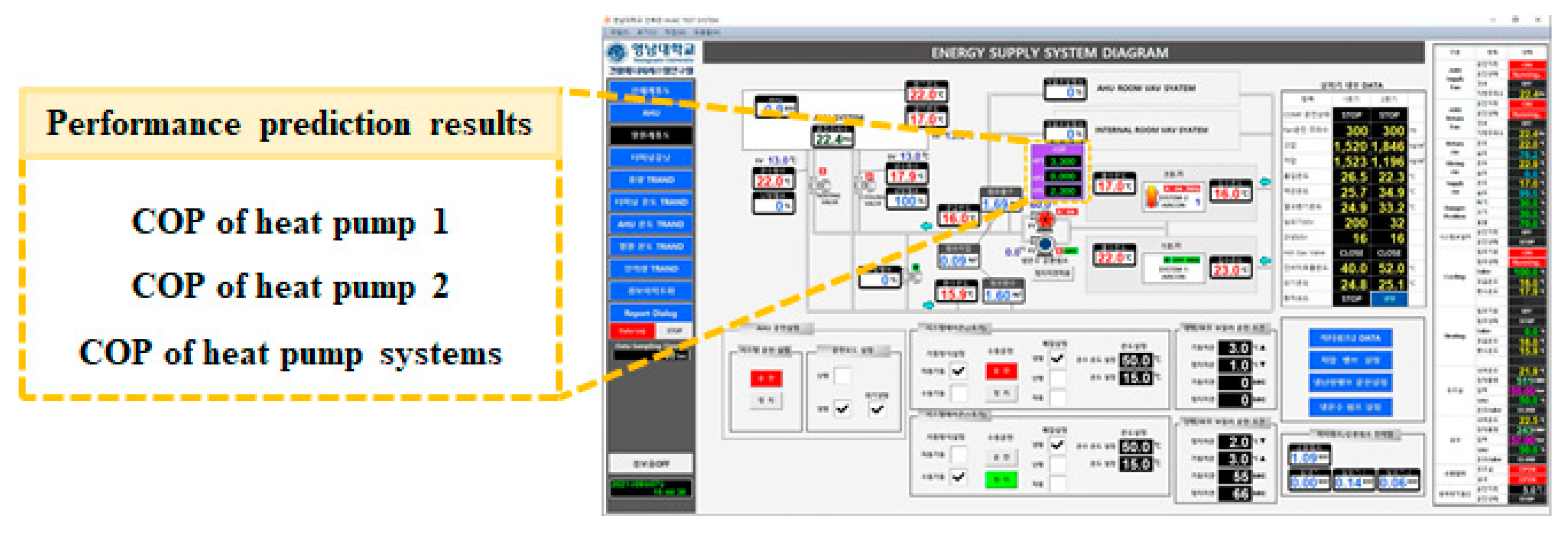
According to the results of the calculation speed and accuracy of the performance prediction model analyzed above, the ANN model showed the highest accuracy and the fastest calculation speed for the data format related to the performance prediction of the heat pump system. To verify the applicability of the developed ANN-based performance prediction model, the performance prediction model was applied to the BAS of the laboratory where the air-cooled heat pump system was installed. The BAS screen is configured to apply the performance prediction model of the heat pump system and monitor the results, and Figure 9 shows the BAS application screen. In BAS, the performance of the two heat pumps and the performance of the heat pump system are confirmed.
Figure 10 shows the results of analyzing the monitored performance as time series data after applying the artificial neural network-based performance prediction model to the BAS. The predictive model enables real-time performance monitoring during heat pump system operation and is saved in Excel file format. It can be used for diagnosis and efficient operation of heat pumps by checking and analyzing performance data during operation.
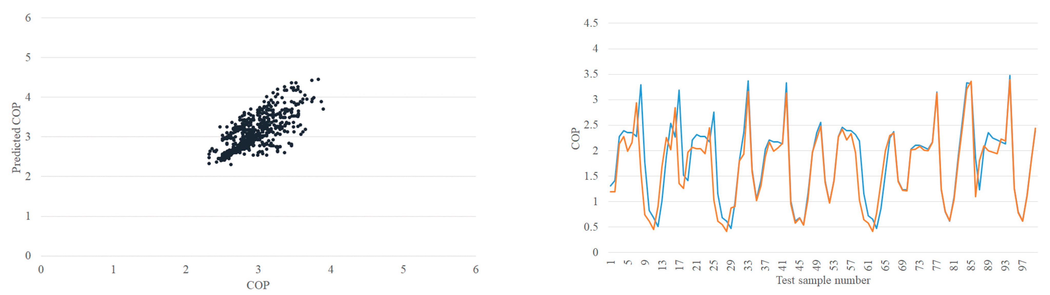
Figure 11 shows the predicted performance monitored by the BAS during the cooling operation period, and the prediction result R2 is 0.9954. Performance changes in the range of about 2.49 to 3.9 were observed during operation of the heat pump system, indicating even predictive performance in all ranges.
It was confirmed that real-time performance prediction and monitoring during system operation was possible through the application of BAS. In the future, the performance degradation of the heat pump system can be checked, and in connection with this, it can be used for system failure diagnosis.
5. Conclusions
In this paper, the performance prediction model was developed and tested using a machine-learning model based on the actual operation data of the air-cooled heat pump system. The performance was predicted using artificial neural networks, support vector machines, random forests, and K-nearest neighbor models, and the accuracy and computation time of the predicted performance were compared. The field applicability was confirmed by applying the developed predictive model to BAS. The detailed conclusion of this paper is as follows.
- (1)
- To develop a predictive model, a university laboratory equipped with an air-cooled heat pump system was selected as a target building and operational data were measured. A statistical analysis was performed between the data and performance collected through the mathematical model and BAS, and through this, the inlet/outlet temperature of the heat source side and the inlet/outlet temperature of the load side were selected as input values.
- (2)
- The training data constructed while developing a predictive model using artificial neural network, support vector machine, random forest, and K-nearest neighbor was subjected to data preprocessing to improve the accuracy of the predictive model. A total of 5124 pieces of data corresponding to 70% of the collected data were used as training data for predictive model development, and 30% of the data (2196 pieces) not used as training data are testing data to verify the performance of the developed model. A predictive model was developed using R studio.
- (3)
- As a result of evaluating the accuracy of the developed performance prediction model, MBE of ANN was −3.6, MBE of SVM was −5, MBE of RF was −7.7, and MBE of KNN was −8.3. This satisfies the verification criteria of ASHRAE Guideline 14 and confirmed that the developed predictive model has excellent performance. ANN with the best accuracy and short computation time among the developed prediction models was applied to the BAS of the laboratory. Real-time performance monitoring is possible through BAS, and the field applicability of the development model was confirmed.
Real-time performance can be checked through the developed performance prediction model, and it can be used for system failure diagnosis and optimal control. When applied to a heat pump system, it can be used as a control point for a heat pump system through prediction of performance that is difficult to predict, and it is expected that energy-saving and performance improvement will be possible.
Author Contributions
All authors contributed to this work. J.-H.S. investigated and wrote the original draft. Y.-H.C. did project administration and supervised. All authors have read and agreed to the published version of the manuscript.
Funding
This research was funded by the National Research Foundation of Korea (NRF) grant funded by the Korea government, grant number NRF-2019R1A2C1009445.
Institutional Review Board Statement
Not applicable.
Informed Consent Statement
Not applicable.
Data Availability Statement
Not applicable.
Conflicts of Interest
The authors declare no conflict of interest.
References
- Solomatine, D.P.; Ostfeld, A. Data-driven modeling: Some past experiences and new approaches. J. Hydroinform. 2008, 10, 3–22. [Google Scholar] [CrossRef] [Green Version]
- Wang, G.; Wang, H.; Kang, Z.; Feng, G. Data-Driven Optimization for Capacity Control of Multiple Ground Source Heat Pump System in Heating Mode. Energies 2020, 13, 3595. [Google Scholar] [CrossRef]
- Zhao, Y.; Li, T.; Zhang, X.; Zhang, C. Artificial intelligence-based fault detection and diagnosis methods for building energy systems: Advantages, challenges and the future. Renew. Sustain. Energy Rev. 2019, 109, 85–101. [Google Scholar] [CrossRef]
- Goodfellow, I.; Bengio, Y.; Courville, A. Deep Learning; MIT Press: Cambridge, MA, USA, 2016; ISBN 0262035618. [Google Scholar]
- Zhang, L.; Wen, J.; Li, Y.; Chen, J.; Ye, Y.; Fu, Y.; Livingood, W. A Review of Machine Learning in Building Load Prediction. Appl. Energy 2021, 285, 116452. [Google Scholar] [CrossRef]
- Mariano-Hernández, D.; Hernández-Callejo, L.; Solís, M.; Zorita-Lamadrid, A.; Duque-Perez, O.; Gonzalez-Morales, L.; Santos-García, F. A Data-Driven Forecasting Strategy to Predict Continuous Hourly Energy Demand in Smart Buildings. Appl. Sci. 2021, 11, 7886. [Google Scholar] [CrossRef]
- Consumption Forecasting in Smart Buildings: Methods, Input Variables, Forecasting Horizon and Metrics. Appl. Sci. 2020, 10, 8323. [CrossRef]
- Bourhnane, S.; Abid, M.R.; Lghoul, R.; Zine-Dine, K.; Elkamoun, N.; Benhaddou, D. Machine Learning for Energy Consumption Prediction and Scheduling in Smart Buildings. SN Appl. Sci. 2020, 2, 297. [Google Scholar] [CrossRef] [Green Version]
- Lopez-Martin, M.; Sanchez-Esguevillas, A.; Hernandez-Callejo, L.; Arribas, J.I.; Carro, B. Novel Data-Driven Models Applied to Short-Term Electric Load Forecasting. Appl. Sci. 2021, 11, 5708. [Google Scholar] [CrossRef]
- Scarpa, M.; Emmi, G.; Carli, M.D. Validation of a numerical model aimed at the estimation of performance of vapor compression based heat pumps. Energy Build. 2012, 47, 411–420. [Google Scholar] [CrossRef]
- Esen, H.; Inalli, M.; Sengur, A.; Esen, M. Performance prediction of a ground-coupled heat pump system using artificial neural networks. Expert Syst. Appl. 2008, 35, 1940–1948. [Google Scholar] [CrossRef]
- Yan, L.; Hu, P.; Li, C.; Yao, Y.; Xing, L.; Lei, F.; Zhu, N. The performance prediction of ground source heat pump system based on monitoring data and data mining technology. Energy Build. 2016, 127, 1085–1095. [Google Scholar] [CrossRef]
- Lu, S.; Li, Q.; Bai, L.; Wang, R. Performance predictions of ground source heat pump system based on random forest and back propagation neural network models. Energy Convers. Manag. 2019, 197, 111864. [Google Scholar] [CrossRef]
- Puttige, A.R.; Andersson, S.; Ostin, R.; Olofsson, T. Application of Regression and ANN Models for Heat Pumps with Field Measurements. Energies 2021, 14, 1750. [Google Scholar] [CrossRef]
- Zendehboudi, A.; Zhao, J.; Li, X. Data-driven modeling of residential air source heat pump system for space heating. J. Therm. Anal. Calorim. 2021, 145, 1863–1876. [Google Scholar] [CrossRef]
- Sun, X.; Wang, Z.; Li, X.; Xu, Z.; Yang, Q.; Yang, Y. Seasonal heating performance prediction of air-to-water heat pumps based on short-term dynamic monitoring. Renew. Energy 2021, 180, 829–837. [Google Scholar] [CrossRef]
- Liu, Q.; Li, N.; Duan, J.; Yan, W. The Evaluation of the Corrosion Rates of Alloys Applied to the Heating Tower Heat Pump (HTHP) by Machine Learning. Energies 2021, 14, 1972. [Google Scholar] [CrossRef]
- Deb, C.; Zhang, F.; Yang, J.; Lee, S.E.; Shah, K.W. A Review on Time Series Forecasting Techniques for Building Energy Consumption. Renew. Sustain. Energy Rev. 2017, 74, 902–924. [Google Scholar] [CrossRef]
- Runge, J.; Zmeureanu, R. A Review of Deep Learning Techniques for Forecasting Energy Use in Buildings. Energy 2021, 14, 608. [Google Scholar] [CrossRef]
- Ruschenburg, J.; Cutic, T.; Herkel, S. Validation of a black-box heat pump simulation model by means of field test results from five installations. Energy Build. 2014, 84, 506–515. [Google Scholar] [CrossRef]
- Amasyali, K.; El-Gohary, N.M. A Review of Data-Driven Building Energy Consumption Prediction Studies. Renew. Sustain. Energy Rev. 2018, 81, 1192–1205. [Google Scholar] [CrossRef]
- ASHRAE. ASHRAE Guideline 14-2014 for Measurement of Energy and Demand Savings; American Society of Heating, Refrigeration and Air Conditioning Engineers: Atlanta, GA, USA, 2014. [Google Scholar]
- ASHRAE. ASHRAE Handbook-Systems and Equipment, Chapter 36; American Society of Heating, Refrigerating and Air-Conditioning Engineers, Inc.: Atlanta, AP, USA, 1996. [Google Scholar]
- ASHRAE. Commercial/Institutional Ground-Source Heat Pumps Engineering Manual; American Society of Heating, Refrigerating and Air-Conditioning Engineers, Inc.: Atlanta, AP, USA, 1995. [Google Scholar]
Figure 1.
Heat pump System. (a) Indoor unit, (b) Outdoor unit.

Figure 2.
Diagram of heat pump system and sensor.

Figure 3.
Diagram of machine-learning model. (a) ANN, (b) SVM, (c) RF, (d) KNN.

Figure 4.
R studio.

Figure 5.
Comparison of predicted and measured performance using ANN model.

Figure 6.
Comparison of predicted and measured performance using SVM model.

Figure 7.
Comparison of predicted and measured performance using RF model.

Figure 8.
Comparison of predicted and measured performance using KNN model.

Figure 9.
BAS application of performance prediction model.

Figure 10.
BAS application and monitoring result of predictive model.

Figure 11.
Comparison of predicted and measured performance.


Table 1.
System configuration.
| Category | System | Number of System |
|---|---|---|
| HVAC system | AHU | 1 |
| VAV terminal unit with reheat coil | 2 | |
| Heat source system | Air-cooled heat pump systems | 2 |
Table 2.
System specification.
| Category | Rated Capacity (kW) | Power Consumption (kW) | |||
|---|---|---|---|---|---|
| Cooling | Heating | Cooling | Heating | ||
| Heat source system | Indoor unit | 4.64 | 5.2.0 | 0.01 | 0.01 |
| Outdoor unit | 4.64 | 5.12 | 30.5 | 29.0 | |
Table 3.
Analysis of input value.
| Input Variable | Non-Standardization Factor | p | ANOVA | |||
|---|---|---|---|---|---|---|
| B | Std. Err | R2 | F | Sig | ||
| Source side input temperature | 8.34 | 1.52 × 10⁻¹⁶ | <0.05 | 0.9023 | 8.44 | <0.001 |
| Source side output temperature | 8.50 | 0.0448 | <0.05 | 0.556 | 104.27 | <0.001 |
| Load side input temperature | 2.96 | 0.0822 | <0.05 | 0.3316 | 167.16 | <0.001 |
| Load side output temperature | 3.62 | 0.1242 | <0.05 | 0.1661 | 8.71 | <0.001 |
Table 4.
Parameter configuration of ANN model.
| Category | Contents | ||
|---|---|---|---|
| Structure | Input layer | Number of layers | 1 |
| Number of neurons | 4 | ||
| Hidden layer | Number of layers | 5 | |
| Number of neurons | 2 | ||
| Output layer | Number of layers | 1 | |
| Number of neurons | 1 | ||
| Function | Activation | Sigmoid | |
| Optimization algorithm | Adam | ||
Table 5.
Parameter configuration of SVM model.
| Category | Contents |
|---|---|
| Kernel function | Gaussian |
| Kernel scale | 1.2 |
| Box constraint level | 1 |
| Standardize data | True |
Table 6.
Parameter configuration of RF model.
| Category | Contents |
|---|---|
| Number of trees | 400 |
| Number of samples at each decision split | 6 |
| Minimum number of samples at leaf | 10 |
Table 7.
Parameter configuration of KNN model.
| Category | Contents |
|---|---|
| Number of neighbors | 3 |
| Distance metric | Euclidean |
Table 8.
Accuracy of prediction model.
| Output | Prediction Model | Accuracy [%] | ||
|---|---|---|---|---|
| MBE | CvRMSE | Error | ||
| Coefficient of Performance | ANN | −3.6 | 5.4 | −7.8~9 |
| SVM | −5.0 | 6.0 | −11~11 | |
| RF | −7.7 | 6.9 | −14~16 | |
| KNN | −8.3 | 8.1 | −12~12 | |
Table 9.
Computation time of prediction model.
| Category | ANN | SVM | RF | KNN |
|---|---|---|---|---|
| Computation time | 31 s | 1 min 20 s | 2 min 8 s | 2 min 22 s |
Publisher’s Note: MDPI stays neutral with regard to jurisdictional claims in published maps and institutional affiliations. |
© 2021 by the authors. Licensee MDPI, Basel, Switzerland. This article is an open access article distributed under the terms and conditions of the Creative Commons Attribution (CC BY) license (https://creativecommons.org/licenses/by/4.0/).
Share and Cite
MDPI and ACS Style
Shin, J.-H.; Cho, Y.-H. Machine-Learning-Based Coefficient of Performance Prediction Model for Heat Pump Systems. Appl. Sci. 2022, 12, 362. https://0-doi-org.brum.beds.ac.uk/10.3390/app12010362
AMA Style
Shin J-H, Cho Y-H. Machine-Learning-Based Coefficient of Performance Prediction Model for Heat Pump Systems. Applied Sciences. 2022; 12(1):362. https://0-doi-org.brum.beds.ac.uk/10.3390/app12010362
Chicago/Turabian StyleShin, Ji-Hyun, and Young-Hum Cho. 2022. "Machine-Learning-Based Coefficient of Performance Prediction Model for Heat Pump Systems" Applied Sciences 12, no. 1: 362. https://0-doi-org.brum.beds.ac.uk/10.3390/app12010362
Note that from the first issue of 2016, this journal uses article numbers instead of page numbers. See further details here.