
Multivariate Wind Turbine Power Curve Model Based on Data Clustering and Polynomial LASSO Regression


1
Department of Engineering, University of Perugia, Via G. Duranti 93, 06125 Perugia, Italy
2
Computer Science Department, University of Exeter, Exeter EX4 4PY, UK
*
Author to whom correspondence should be addressed.
Appl. Sci. 2022, 12(1), 72; https://0-doi-org.brum.beds.ac.uk/10.3390/app12010072
Submission received: 17 November 2021
/
Revised: 13 December 2021
/
Accepted: 21 December 2021
/
Published: 22 December 2021
(This article belongs to the Special Issue Wind Generators: Technology and Trends)
Abstract
:Featured Application
Wind turbine performance monitoring through a computationally affordable method.
Abstract
Wind turbine performance monitoring is a complex task because of the non-stationary operation conditions and because the power has a multivariate dependence on the ambient conditions and working parameters. This motivates the research about the use of SCADA data for constructing reliable models applicable in wind turbine performance monitoring. The present work is devoted to multivariate wind turbine power curves, which can be conceived of as multiple input, single output models. The output is the power of the target wind turbine, and the input variables are the wind speed and additional covariates, which in this work are the blade pitch and rotor speed. The objective of this study is to contribute to the formulation of multivariate wind turbine power curve models, which conjugate precision and simplicity and are therefore appropriate for industrial applications. The non-linearity of the relation between the input variables and the output was taken into account through the simplification of a polynomial LASSO regression: the advantages of this are that the input variables selection is performed automatically. The k-means algorithm was employed for automatic multi-dimensional data clustering, and a separate sub-model was formulated for each cluster, whose total number was selected by analyzing the silhouette score. The proposed method was tested on the SCADA data of an industrial Vestas V52 wind turbine. It resulted that the most appropriate number of clusters was three, which fairly resembles the main features of the wind turbine control. As expected, the importance of the different input variables varied with the cluster. The achieved model validation error metrics are the following: the mean absolute percentage error was in the order of 7.2%, and the average difference of mean percentage errors on random subsets of the target data set was of the order of 0.001%. This indicates that the proposed model, despite its simplicity, can be reliably employed for wind turbine power monitoring and for evaluating accumulated performance changes due to aging and/or optimization.
1. Introduction
Wind power is currently considered as the most promising source of renewable electricity in the world. Nevertheless, due to the non-stationary conditions to which wind turbines are subjected, performance monitoring and early fault diagnosis are non-trivial tasks. For this reason, despite wind turbines’ substantially constituting a mature technology, the O&M costs can still reach the order of 25% of the overall life-cycle costs [1,2].
In the wind energy practitioners’ community, the standard for the evaluation of wind turbine performance is the analysis of the power curve, i.e., the curve displaying the relation between the wind flow intensity and the power output: the IEC recommends the binning method [3], consisting of averaging the power measurement per wind speed intervals of 0.5 m/s or 1 m/s. In general, the averaging or discretisation of wind turbine data [4] provides meaningful indications. The power curve analysis has the great advantage of simplicity, but the drawback is that it does not account for the fact that the power of a wind turbine has a multivariate dependence on the environmental conditions and working parameters [5]. Furthermore, the undisturbed wind flow is not measured directly: it is estimated through a nacelle transfer function based on downwind measurements collected behind the rotor span [6,7,8].
The widespread diffusion of Supervisory Control And Data Acquisition (SCADA) has been a turning point and has projected wind energy into the era of data. SCADA systems record a vast set of environmental, operational, mechanical, electrical, and thermal data with a frequency in the order of Hertz and store them upon averaging with a time basis of a few minutes (typically ten). Wind turbine performance monitoring and fault diagnosis have been therefore gradually evolving into data analysis problems: the general concept is that anomalous performance or incoming damages are individuated by analyzing the residuals between the measurements and data-driven normal behavior model [9,10,11,12,13,14,15,16,17]. The critical points as regards this kind of approach are repeatability, generalization, supervision, and absence of theoretical standards, and the literature is focused on these aspects. Given these considerations, also the study of wind turbine power curves has become substantially a problem of data analysis and interpretation [18,19,20,21,22,23,24].
A recent line of research about wind turbine power curves regards multivariate approaches [25,26,27,28,29,30,31]: the general idea is that the power of a wind turbine is the output of a data-driven model, which has further input variables in addition to the wind speed. Despite it have been shown that the wind speed can account for up to the 99% of the variance of the power [32] and therefore further input variables can explain not more than the residue of 1%, this can be decisive in order to obtain data-driven models whose average error metrics are sufficiently low to guarantee a robust monitoring of wind turbine performance. For a recent review about multivariate wind turbine power curves, refer to [33].
From the discussion in [33], it arises that the literature about wind turbine multivariate power curves is at its early stages, but some evidence has been gradually accumulating:
- Due to the complexity of the wind flow at the microscale level, meteorological mast data can be useful only for modeling the power of a wind turbine that is sited extremely close to the mast [6]. For application in real-world large wind farms, meteorological mast data are not appropriate for wind turbine power curve models [34];
- Consequently, the most meaningful additional input variables for modeling the power of a wind turbine are the working parameters.
In regard to the latter point, the blade pitch and the rotational speed have been individuated as the most relevant operation variables to be employed in a multivariate wind turbine power curve model. This is definitely reasonable, given that the theoretical expectation is that the power of a wind turbine is (Equation (1)):
In Equation (1), P is the produced power and depends on the rotor radius R, the air density , the wind speed v, and the power factor , which depends on the blade pitch angle and the tip-speed ratio (or, in other words, the rotational speed ). The role of the rotational speed and blade pitch in data-driven models for the power was explored in detail in [5]: in that study, the rotor speed and blade pitch were added once at a time to a Gaussian process regression for the power of a wind turbine. The main result was that the inclusion of both variables reduced the error metrics and the rotational speed was slightly more influential than the blade pitch. The use of these two variables was discussed also in [29,31,35].
A further relevant technical development for multivariate wind turbine power curve models is data clustering [36]. Actually, it is likely that employing more than one sub-model might be more convenient than employing one model for all the power curve span. This is reasonable, because between the cut-in and the rated wind speed, it is possible to distinguish three operation regions, which have different features:
- Near the cut-in (approximately between 3 m/s and 5 m/s of wind intensity), the rotational speed of a wind turbine is practically fixed and the blade pitch varies;
- In the full aerodynamic load region (approximately between 5 m/s and 9 m/s of wind speed), the wind turbine attains the maximum possible aerodynamic efficiency by varying the rotational speed and holding the blade pitch practically fixed;
- In the partial aerodynamic load region (approximately above 9 m/s of wind intensity), the rotational speed is held fixed at the rated speed and the load is varied by regulating the blade pitch.
Based on these considerations, the objective of the present study is formulating a multivariate method for data-driven wind turbine power curve analysis, which can be easily implemented in industrial applications. Therefore, each building block of a good multivariate wind turbine power curve model was simplified as much as possible. This was performed as follows:
- The selection of the input variables was drastically simplified. Based on considerations similar to [5], the selected covariates of the model are wind speed, blade pitch, and rotor speed;
- The structure of the model was selected according to a compromise. It is evident that a linear model would be too simple: this was observed also in the recent study [31]. Nevertheless, it is worth exploring if it is possible to account for non-linearity in a simplified way, namely through a polynomial in the above indicated input variables. Therefore, a polynomial LASSO regression was selected. The advantage of this kind of model structure is that a selection of the covariates is substantially performed when the coefficients of the polynomial are set. A covariate, which was excluded from the model, has a vanishing coefficient in the polynomial;
- The data clustering was performed using the k-means algorithm on a reference data set: it was selected because it is a very well-established method, which can easily be implemented in industrial applications. The number of clusters was set automatically by computing the average silhouette score for each cluster number arrangement.
The peculiarity and the innovativeness of the present study can therefore be individuated in a complex application (data-driven multivariate wind turbine power curve), characterized by several critical points, which must be mastered in depth, in order to provide solutions to each building block of the problem, which can be as simple as possible. This approach is novel in the scientific literature, because the applications of data clustering and non-linear multivariate power curves are at their early stages, and it is interesting for the industry because the use of data-driven models for custom wind turbine performance monitoring has been gradually becoming a necessity. The general structure of the method is summarized in the workflow of Figure 1.
The study is organized as a test case discussion, based on the analysis of the SCADA data of a Vestas V52 wind turbine sited in Italy (850 kW rated power): the data were provided by the Lucky Wind company. Practically, the goodness of the proposed approach is discussed through the analysis of the most common performance metrics (MAE, MAPE, RMSE) for the validation of the data-driven model. Furthermore, a method for analyzing the accumulated performance change is proposed: it is based on the analysis of how the MAPE changes in two subsets of the target data set. This procedure is useful in the applications for individuating small performance changes accumulated along a relatively long period: this can happen in the form of performance improvement due to technology optimizations [37] or, vice versa, in the form of performance worsening [38,39], which can occur due to the aging of the machine.
2. The Test Case and the Data Sets
The wind turbine of interest is sited in Italy and the model type is Vestas V52. The rated power is 850 kW; the cut-in wind speed is 4 m/s; the rated wind speed is 14 m/s. The rotor diameter is 52 m.
Two data sets were employed:
- goes from 1 January 2019 to 31 December 2019;
- goes from 1 January 2020 to 31 December 2020.
The available validated measurements have 10 min of sampling time, and those at disposal for the present study are:
- Produced power P;
- Undisturbed wind speed reconstructed by the nacelle anemometer;
- Rotor speed ;
- Blade pitch ;
- Ambient temperature T.
The data pre-processing was based on the following steps, which are easily replicable in industrial applications:
- The data were filtered on the wind turbine’s normal operation using the appropriate runtime counter provided by the SCADA system;
- Industrial wind farms rarely operate under curtailment dictated by grid requirements, and this is the case also for the present wind turbine. This aspect has nothing to do with wind turbine performance, and therefore, operation under curtailment should be filtered out for the purposes of the present work. This can be done by noticing that a wind turbine operates in derated conditions by pitching anomalously with respect to the normal. Therefore, the average wind speed/blade pitch [40] can be used for individuating outliers associated with derating. The filtering can be practically performed by eliminating time steps where the blade pitch deviates more than a threshold ( in this study) with respect to the average blade pitch for the given wind speed;
- For each wind turbine, data were filtered between cut-in and the rated speed because the power monitoring becomes trivial above the rated speed.
Upon filtering, constitutes 18,000 samples and 19,930 samples. A summary of the features of the data sets is reported in Table 1.
The dependence of wind turbine power on environmental conditions is a widely debated issue, in particular as regards the external temperature [41]. Given the applied point of view of the present study, the simplest method was selected: it consists of the renormalization of by considering the effect of air density as indicated in Equations (2) and (3):
where is the corrected wind speed, is the air density measured on site, is the air density in standard conditions, is the absolute temperature in standard conditions (288.15 K), and T is the absolute ambient temperature measured on site.
An example of the raw data set and of the pre-processed data set (resulting in ) is reported in Figure 2.
3. Methods
3.1. General Description
As supported also by Figure 1, the proposed method involves a complex framework because two data sets were employed for the training and application of clustering and regression. The peculiarity of this work is that each building block of this complex problem was simplified as much as possible, given the knowledge of the critical points of multivariate data-driven wind turbine power curve models and of the limits within which simplifying is acceptable.
In summary, the steps of the method are the following:
- Divide into clusters using the k-means algorithm, with ;
- For each k, compute the average silhouette score;
- Select the value of k that gives the highest average silhouette score;
- Apply the k-means algorithm to the data set , using the value of k selected above and using the corresponding centroids C as initial values;
- For each cluster of the data set, train a LASSO regression and fix the hyperparameters and the coefficients through K-fold cross-validation (with k = 10);
- For each cluster of the data set, simulate the output using the corresponding regression trained with the data;
- Compute the error metrics by elaborating the difference between the measurements and estimations on the data set.
3.2. Data Clustering
The data set was divided into clusters based on the well-known k-means algorithm [42]. This algorithm has been selected because it can be easily implemented in industrial applications using most statistical packages. Furthermore, the drawbacks of the algorithm are mitigated for the present applications: severe outliers are filtered out in the pre-processing phase, and therefore, the centroids selection should be reliable; furthermore, the dimensionality issue is contained by the fact the selected possible covariates are nine (Table 1). It should be noticed that the literature on the application of clustering algorithms to multivariate wind turbine power curves is at its early stages; for example, the k-means algorithm was applied in the recent paper [43] and a more sophisticated fuzzy clustering was applied in [44]. Based on these considerations, it was considered of interest for the purposes of the present study to apply the k-means algorithm, but it is clear that the applications of smarter methods (as hierarchical clustering [45,46]) would be a valuable step forward.
The algorithm starts from N possibly multi-dimensional observations , and the objective is partitioning the observations into k groups in order to minimize the within-cluster sum of squares (variance), as indicated in Equation (4):
where is the data partitioning and is the data average in the i-th partition. The standard algorithm starts from an initial set of k means and assigns each observation to the cluster having less distance with respect to the mean: for each observation addition, the centroids (i.e., the means) are re-computed, and the algorithm stops when the assignments no longer change.
In this study, the selection of the number of clusters was performed automatically through the analysis of the silhouette score [47]. For each i-th observation associated with the j-th cluster, the silhouette score is defined in Equation (2):
where is the mean distance between the i-th observation and all the other data points in the same cluster and is the minimum of the mean distances between the i-th observation and all the points for each other cluster. and were computed using the Euclidean distance, but there are other possible choices that have been explored in the literature [48,49]. Given the definition in Equation (2), it arises that : approaching one means that the observation is well associated with a cluster; approaching −1 means that the observation should rather be assigned to a neighboring cluster. The silhouette coefficient for a given clustering of the observations can be computed as the average of the silhouette scores (Equation (2)) over all the observations.
In this study, k ranging from 2–20 was contemplated, and the configuration with the highest silhouette coefficient was selected: this procedure was applied on the reference data set, and the obtained centroids were fed as input for the clustering of (with the same number of clusters as ).
3.3. Polynomial LASSO Regression
Given M covariates , with , the LASSO regression is a particular way of establishing a multivariate linear model (Equation (5)) between the set of and the target y.
In this study, a model for each of the k clusters was set using the reference data set. The target of the models is the power P of the test case wind turbine, and the covariates are listed in Table 2: the set of covariates includes the wind speed , the blade pitch , and the rotor speed up to third power. This was done because the relation between the wind speed and the power is non-linear, and it can be approximated as cubic at least in a part of the power curve; furthermore, it is known that the power factor of a wind turbine depends non-linearly on the blade pitch [38]. Therefore, the objective of the present regression structure is inquiring if it is possible to approximate with a polynomial the non-linear dependence of the power P on the wind speed and on the most influential working parameters (blade pitch and rotor speed ).
The LASSO regression algorithm selects the coefficients by adding one covariate at a time, so that the added covariate has the highest correlation with the target y. The coefficients are set by minimizing the cost function in Equation (6):
where is the number of observations in the training data set and the estimation is given in Equation (7):
The LASSO regression, expressed in terms of the covariates, is basically a multivariate linear regression where the coefficients are set by minimizing the squared sum of errors with a bound on the norm of the coefficients of the regression. The rationale for selecting this method in the present work is that the penalty on the norm of the coefficients (Equation (6)) forces the coefficients of the covariates having a minor contribution to the model to be exactly zero: this substantially acts as a simple feature selection algorithm, which can easily be implemented in applications, and this is the reason why this was considered appropriate for the purposes of the present work.
To set the hyperparameter , k-fold (with k = 10) cross-validation was performed [50]. Equation (7) was employed for simulating the output on the target data set , and the performance of the model, given the residuals between the model estimated and measurements (Equation (8)), was quantified through the most common metrics: (Equation (9)), (Equation (10)), and (Equation (11)).
where is the number of observations in the data set and is the average residual, which is given in Equation (12):
The metrics in Equations (9)–(11) can be computed on the whole data set or separately for each of the k clusters and provides an estimate of the average model precision in simulating each single measurement of power P. Since the performance changes of a wind turbine can be very small (order of a percent or less of the power P) and can be due to control and technology optimization [37] or, vice versa, to aging effects [38], it can be practically of interest to understand the capability of the model in detecting a small accumulated effect along a large data set.
For this reason, following [51,52], one can divide the data set into two subsets (indicated with subscripts 1 and 2) and compute the quantity in Equation (13):
Since, to the knowledge of the wind turbine owner and of the authors, there have been no events at the test case wind turbine during , was theoretically expected to be vanishing, and therefore, the obtained results for can be interpreted as the sensitivity of the model, i.e., a lower bound on the accumulated performance change that can be detected. The subdivision of into two random subsets can be performed an arbitrary number of times, and can be computed for each time and averaged on the runs (thus obtaining a as in Equation (14)): runs were selected for this study.
4. Results
4.1. Data Clustering
In Figure 3, the average silhouette score for the clustering of the data set is reported, with the number of clusters k ranging from 2–20; given this, the selected number of clusters is three.
In Figure 4, the best-performing clustering (silhouette coefficient equal to 0.84) of the reference data set is reported in the power curve plot. It arises that the clustering fairly resembles the operation regions: near cut-in (pitch control), full load region (fixed pitch and variable rotor speed), and partial load region (pitch control and fixed rotor speed). In Figure 5, the corresponding plot for the data set is reported: the clusters are set starting from the centroids computed for the data set .
It is evident that Figure 4 and Figure 5 are qualitatively very similar. In order to have a deeper insight into this aspect, the k-means algorithm with three clusters was run independently on the data set , and this classification was compared against the one obtained by starting with the centroids of the D1 data set. It arises that these two classifications coincide up to 96%, but this is not guaranteed if the method of this work is extended to a higher number of covariates.
4.2. Polynomial LASSO Regression
In Table 3, the coefficients of the LASSO regression are reported: as indicated in Section 3.3, they were computed from the reference data set . It is interesting to notice that for Cluster 1, there is a weak dependence of the power P on the rotor speed , and this is consistent because the wind turbine basically operates at a fixed rotor speed in that region. As regards Cluster 3, the coefficient of the covariate was set to zero, which is reasonable because, near the rated power, the power P grows more slowly than .
The results for the K-fold cross-validation for the three clusters are reported in Table 4, in the form of the average RMSE and associated standard deviation. From Table 4, the proposed model behaved better in the near-rated region (Cluster 3) with respect to the moderate wind intensity region of Cluster 2: this is a non-trivial result because in previous studies [31], it has been highlighted that the near-rated regime is particularly critical to simulate.
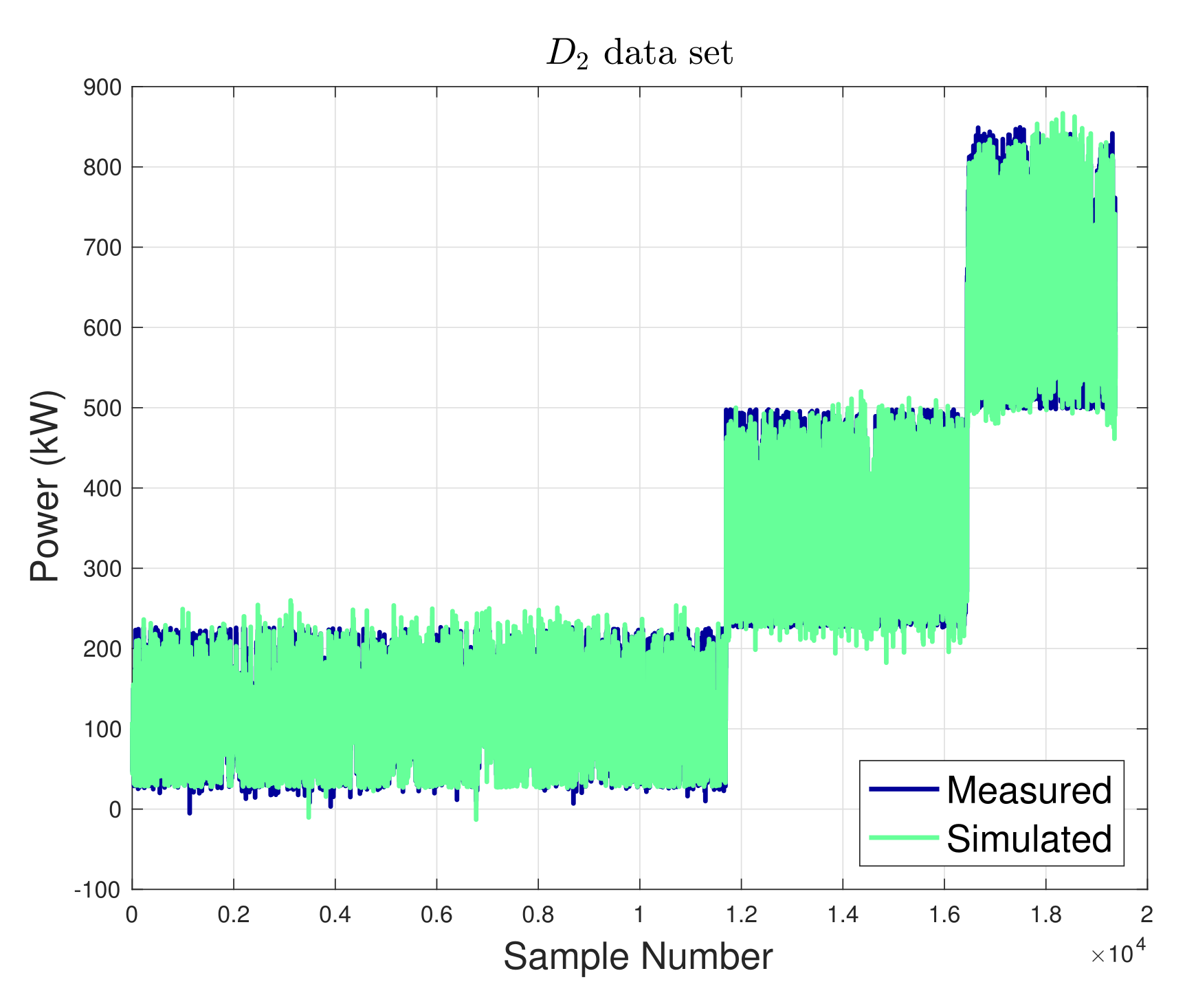
In Figure 6, the measured and simulated data are reported, grouped into clusters. Figure 7 reports a zoom on an excerpt of the data from Figure 6, in order to appreciate the capability of the model in reproducing the behavior of the measured data.
In Table 5, the results are reported as regards the model errors when simulating the output on the target data set : the main result is that on average, the single measurement of the power P can be simulated with a 7.2% percentage error. An interesting aspect is that the absolute errors do not increase from Cluster 2 to Cluster 3 and decrease in percentage (up to 2.8% on average), consistent also with Table 4; this is noticeable because, typically, the most challenging operation region for modeling the power P is the near-rated power (as discussed for example in [31]). The overall result for the is noticeable as well, because it means that the power P can on average be predicted with an absolute error of 12 kW, which is 1.4% of the rated power of the test case wind turbine.
Figure 8 allows a visualization of the model properties depending on the operation regime: it consists o the plot (for data set ) of the residuals R (Equation (8)), averaged in intervals of measured power P whose amplitude is 10% of the rated. The average absolute residual was in general of the order of 5 kW and increased at the crossroad between Cluster 2 and Cluster 3; this is reasonable because, in this region, the wind turbine control switches from variable rotor speed and fixed pitch to rated rotor speed and pitch control. It is reasonable that the weak point of the proposed method is cluster merging; multi-dimensional measurements at the crossroad of two clusters should likely be assigned partially to both of them, for example through a fuzzy membership function. Nevertheless, this was considered out of the scope of the present study because simple methods, easily implementable in the industry, were selected.
Table 6 reports the results for the average difference of when dividing into two random subsets: this procedure was applied to the whole data set and separately for each cluster. These results clearly indicate that the proposed method is appropriate for detecting accumulated performance changes with a high sensitivity: this can be particularly useful for analyzing wind turbine aging and/or retrofitting.
4.3. Comparison against Benchmark Models
In order to support the usefulness of the approach proposed in this work, in this subsection, the comparison against benchmark models is pursued. The same kind of procedure is adopted, as depicted in Figure 1: the unique difference is given by the fact that the LASSO regression of Section 3.3 is substituted by other types of regression. For brevity, the reported information about this benchmark regressions is essential, since the selected models are well known in the literature.
The benchmark models are the following:
- Univariate LASSO: For each cluster, a LASSO regression similar to the one in Section 3.3 was set up. The set of possible covariates from which the regression starts is given by . Given that, as supported also in [32], the wind speed is the most important input variable for a power curve model; this benchmark was selected in order to analyze how much improvement is obtained when the same kind of regression is maintained and the most important operation variables are included (as in Section 3.3);
- Multivariate support vector regression: This benchmark is obtained by setting up a multivariate SVR for each cluster. The input variables are the corrected wind speed , the blade pitch , and the rotor speed . In this case, the non-linearity is accounted for implicitly by the model, and there is no relevance in feeding as the input higher powers of the input variables;
- Multivariate Gaussian process regression: This benchmark is similar as the previous, but the regression is based on the Gaussian process.
The two multivariate benchmarks were selected because they have been widely employed for multivariate wind turbine power curve models [5,18,31], and it is therefore interesting to inquire to what extent the error metrics worsen when the simplifications of this work are adopted.
The results for univariate LASSO are reported in Table 7. Comparing against Table 5, the overall and were one third higher, and this was due mainly to the increased errors in Clusters 2 and 3, for moderate and high wind speeds.
The results for the multivariate SVR and GPR are reported respectively in Table 8 and Table 9 and were quite similar. By comparing against Table 5, the overall and were lower for the model proposed in this work; this is a remarkable result, given the simplification of the LASSO regression of Section 3.3. The unique substantial advantage of the multivariate SVR and GPR was a lower overall , and this was likely due to the behavior of the models in Cluster 1, where the average power was lower.
In general, the comparison of Table 5, Table 7, Table 8 and Table 9 indicates that there was a substantial improvement provided by the multivariate models with respect to the univariate one. Furthermore, the comparison between the multivariate models indicated that there were no evident error metrics worsening due to the simplifications of the regression proposed in this work.
5. Conclusions and Further Directions
In the present study, a method for multivariate wind turbine power monitoring was proposed. The objective was conjugating simplicity, which can be exploited in industrial applications, with the awareness of the critical points regarding wind turbine multivariate power curves. Actually, in the present study, a meaningful simplified solution was proposed for the following points:
- Set of covariates: The method employs wind speed, blade pitch, and rotor speed and accounts for the dependence on the external temperature by renormalizing the wind speed;
- Model structure: The non-linearity was taken into account through the simplification of a polynomial up to cubic terms in the above-listed input variables. A LASSO regression was performed, which allows formally maintaining the structure of a linear regression;
- Input variables’ selection: Through the K-fold cross-validation of the LASSO regression, the irrelevant input variables were discarded by setting to zero the corresponding coefficient in the polynomial;
- Data clustering: The well-established k-means algorithm was employed to divide the multi-dimensional data appropriately, and a separate sub-model was set up for each cluster.
The method was tested on real-world data from a Vestas V52 wind turbine owned by the Lucky Wind company and sited in Southern Italy. The reference data set was employed for training the k-means algorithm and selecting the optimal data clustering (based on the silhouette coefficient): was selected, and this qualitatively coincides with the main different control regions of a modern wind turbine. Subsequently, a polynomial LASSO regression for the power of the wind turbine was performed for each obtained cluster: the reference data were used for selecting the input variables and setting the regression coefficients through the K-fold cross-validation. The performance of the model was quantified by analyzing the discrepancy between the measurement and simulation in the target data set.
It resulted that the mean absolute error of the model in the validation data set was 12 kW (1.4% of the rated power), corresponding to a mean absolute percentage error of 7.2%. The absolute errors did not increase in the near-rated region with respect to the moderate wind speed region (Cluster 3 against Cluster 2), and therefore, the percentage errors decreased, reaching 2.8% on average. This result is interesting because it is typical that, vice versa, the near-rated region is the most critical as regards power monitoring. It was noticeable that, despite the simplifications of the proposed methods, the obtained average error metrics were competitive with the state-of-the-art in the literature, as can be argued by the discussion in Section 4.3 and by comparing against Table 1 in [33].
Furthermore, an analysis was devoted to monitoring the accumulated performance. The rationale for this analysis was that the order of magnitude of some performance changes possibly occurring in a wind turbine’s lifetime is particularly small, but affects all the observations from a given moment. Therefore, monitoring small performance changes along long periods requires shifting the focus to the difference accumulated in a period against a reference one. To this aim, the target data set considered in this study was randomly split in two, and it was observed that the proposed method had a remarkably high sensitivity because the average accumulated percentage difference that it is possible to detect was of the order of 0.001%.
Therefore, the main lesson from this study, which can be particularly useful in the wind energy practitioners community, is that for application purposes, a multivariate wind turbine power curve model does not need to be overly complicated, but should rather contribute intelligently to each of the critical points regarding this type of problem.
The approach of this work was mainly methodological, but it should be emphasized that it has several practical applications. For example, a similar, albeit more complex method, was employed in [38,53] for quantifying the effect of aging on wind turbine performance. A further application of the present study, which is being pursued at present, is the estimation of the effects of icing on wind turbine performance. Actually, the increasing exploitation of wind energy in harsh environments due to increasing demand for renewable energy production has been posing the issue of characterizing the performance of wind turbines in extreme conditions. Blade icing can likely be individuated as reduced rotor speed, and consequently extracted power, for a given wind speed [54,55,56]: therefore, a model similar to the one proposed in the present paper should be useful to individuate the behavior of a wind turbine in icing conditions.
Furthermore, a topic that has been recently attracting attention in the wind energy literature is the effect of static and dynamic yaw error on wind turbine performance [57,58,59,60]; the incorporation of such an effect in multivariate wind turbine power curve models would be a valuable development. Finally, a useful remark is that the the number of possible covariates could be enlarged quite arbitrarily; in that case, a dimension reduction algorithm such as principal component analysis [61] should be included in the modeling chain.
Author Contributions
Conceptualization, D.A. and R.P.; data curation, D.A.; formal analysis, D.A. and R.P.; investigation, D.A. and R.P.; methodology, D.A.; project administration, D.A.; software, D.A.; supervision, D.A. and R.P., validation, D.A. and R.P.; writing—original draft, D.A.; writing—review and editing, R.P. All authors have read and agreed to the published version of the manuscript.
Funding
This research received no external funding.
Acknowledgments
The authors thank the company Lucky Wind s.p.a. for the technical support and for providing the data sets employed for the study.
Conflicts of Interest
The authors declare no conflict of interest.
Nomenclature
The following abbreviations are used in this manuscript:
| Abbreviation | Meaning |
| GPR | Gaussian Process Regression |
| IEC | International Electrotechnical Commission |
| LASSO | Least Absolute Shrinkage and Selection Operator |
| MAE | Mean Absolute Error |
| MAPE | Mean Absolute Percentage Error |
| MSE | Mean Squared Error |
| O&M | Operation and Maintenance |
| RMSE | Root Mean Squared Error |
| SCADA | Supervisory Control And Data Acquisition |
| SVR | Support Vector Regression |
| Symbol | Meaning |
| k | Number of clusters |
| C | Centroids of the clusters |
| s | Silhouette score |
| y | Output of the regression (measured) |
| Output of the regression (estimated) | |
| Input of the regression | |
| Coefficients of the regression | |
| Hyperparameter of the regression | |
| N | Number of data points |
| K | Number of folds |
| Symbol | Meaning |
| Wind speed measured by nacelle anemometer | |
| Wind speed renormalized with the external temperature (Equations (2) and (3)) | |
| T | External temperature |
| Blade pitch angle | |
| Rotor speed |
References
- Carroll, J.; McDonald, A.; McMillan, D. Failure rate, repair time and unscheduled O&M cost analysis of offshore wind turbines. Wind Energy 2016, 19, 1107–1119. [Google Scholar]
- Ioannou, A.; Angus, A.; Brennan, F. A lifecycle techno-economic model of offshore wind energy for different entry and exit instances. Appl. Energy 2018, 221, 406–424. [Google Scholar] [CrossRef]
- IEC. Power Performance Measurements of Electricity Producing Wind Turbines; Technical Report 61400–12; International Electrotechnical Commission: Geneva, Switzerland, 2005. [Google Scholar]
- Dhont, M.; Tsiporkova, E.; Boeva, V. Advanced Discretisation and Visualisation Methods for Performance Profiling of Wind Turbines. Energies 2021, 14, 6216. [Google Scholar] [CrossRef]
- Pandit, R.K.; Infield, D.; Kolios, A. Gaussian process power curve models incorporating wind turbine operational variables. Energy Rep. 2020, 6, 1658–1669. [Google Scholar] [CrossRef]
- St Martin, C.M.; Lundquist, J.K.; Clifton, A.; Poulos, G.S.; Schreck, S.J. Atmospheric turbulence affects wind turbine nacelle transfer functions. Wind Energy Sci. 2017, 2, 295. [Google Scholar] [CrossRef] [Green Version]
- Carullo, A.; Ciocia, A.; Malgaroli, G.; Spertino, F. An Innovative Correction Method of Wind Speed for Efficiency Evaluation of Wind Turbines. Acta IMEKO 2021, 10, 46–53. [Google Scholar] [CrossRef]
- Spertino, F.; Di Leo, P.; Ilie, I.S.; Chicco, G. DFIG equivalent circuit and mismatch assessment between manufacturer and experimental power-wind speed curves. Renew. Energy 2012, 48, 333–343. [Google Scholar] [CrossRef]
- Yang, W.; Court, R.; Jiang, J. Wind turbine condition monitoring by the approach of SCADA data analysis. Renew. Energy 2013, 53, 365–376. [Google Scholar] [CrossRef]
- Castellani, F.; Garinei, A.; Terzi, L.; Astolfi, D.; Gaudiosi, M. Improving windfarm operation practice through numerical modeling and supervisory control and data acquisition data analysis. IET Renew. Power Gener. 2014, 8, 367–379. [Google Scholar] [CrossRef]
- Schlechtingen, M.; Santos, I.F.; Achiche, S. Wind turbine condition monitoring based on SCADA data using normal behavior models. Part 1: System description. Appl. Soft Comput. 2013, 13, 259–270. [Google Scholar] [CrossRef]
- Li, J.; Lei, X.; Li, H.; Ran, L. Normal behavior models for the condition assessment of wind turbine generator systems. Electr. Power Compon. Syst. 2014, 42, 1201–1212. [Google Scholar] [CrossRef]
- Vidal, Y.; Pozo, F.; Tutivén, C. Wind turbine multi-fault detection and classification based on SCADA data. Energies 2018, 11, 3018. [Google Scholar] [CrossRef] [Green Version]
- Schlechtingen, M.; Santos, I.F. Wind turbine condition monitoring based on SCADA data using normal behavior models. Part 2: Application examples. Appl. Soft Comput. 2014, 14, 447–460. [Google Scholar] [CrossRef]
- Gonzalez, E.; Stephen, B.; Infield, D.; Melero, J.J. Using high-frequency SCADA data for wind turbine performance monitoring: A sensitivity study. Renew. Energy 2019, 131, 841–853. [Google Scholar] [CrossRef] [Green Version]
- Jin, X.; Xu, Z.; Qiao, W. Condition monitoring of wind turbine generators using SCADA data analysis. IEEE Trans. Sustain. Energy 2020, 12, 202–210. [Google Scholar] [CrossRef]
- Natili, F.; Daga, A.P.; Castellani, F.; Garibaldi, L. Multi-Scale Wind Turbine Bearings Supervision Techniques Using Industrial SCADA and Vibration Data. Appl. Sci. 2021, 11, 6785. [Google Scholar] [CrossRef]
- Pandit, R.; Kolios, A. SCADA data-based support vector machine wind turbine power curve uncertainty estimation and its comparative studies. Appl. Sci. 2020, 10, 8685. [Google Scholar] [CrossRef]
- Hu, Y.; Qiao, Y.; Liu, J.; Zhu, H. Adaptive confidence boundary modeling of wind turbine power curve using SCADA data and its application. IEEE Trans. Sustain. Energy 2018, 10, 1330–1341. [Google Scholar] [CrossRef]
- Long, H.; Wang, L.; Zhang, Z.; Song, Z.; Xu, J. Data-driven wind turbine power generation performance monitoring. IEEE Trans. Ind. Electron. 2015, 62, 6627–6635. [Google Scholar] [CrossRef]
- Morrison, R.; Liu, X.; Lin, Z. Anomaly detection in wind turbine SCADA data for power curve cleaning. Renew. Energy 2021, 184, 473–486. [Google Scholar] [CrossRef]
- Guo, P.; Infield, D. Wind turbine power curve modeling and monitoring with Gaussian Process and SPRT. IEEE Trans. Sustain. Energy 2018, 11, 107–115. [Google Scholar] [CrossRef] [Green Version]
- Delgado, I.; Fahim, M. Wind Turbine Data Analysis and LSTM-Based Prediction in SCADA System. Energies 2021, 14, 125. [Google Scholar] [CrossRef]
- Ferguson, D.; McDonald, A.; Carroll, J.; Lee, H. Standardisation of wind turbine SCADA data for gearbox fault detection. J. Eng. 2019, 2019, 5147–5151. [Google Scholar] [CrossRef]
- Schlechtingen, M.; Santos, I.F.; Achiche, S. Using data-mining approaches for wind turbine power curve monitoring: A comparative study. IEEE Trans. Sustain. Energy 2013, 4, 671–679. [Google Scholar] [CrossRef]
- Lee, G.; Ding, Y.; Genton, M.G.; Xie, L. Power curve estimation with multivariate environmental factors for inland and offshore wind farms. J. Am. Stat. Assoc. 2015, 110, 56–67. [Google Scholar] [CrossRef] [Green Version]
- Pelletier, F.; Masson, C.; Tahan, A. Wind turbine power curve modeling using artificial neural network. Renew. Energy 2016, 89, 207–214. [Google Scholar] [CrossRef]
- Manobel, B.; Sehnke, F.; Lazzús, J.A.; Salfate, I.; Felder, M.; Montecinos, S. Wind turbine power curve modeling based on Gaussian processes and artificial neural networks. Renew. Energy 2018, 125, 1015–1020. [Google Scholar] [CrossRef]
- Shetty, R.P.; Sathyabhama, A.; Pai, P.S. Comparison of modeling methods for wind power prediction: A critical study. Front. Energy 2020, 14, 347–358. [Google Scholar] [CrossRef]
- Karamichailidou, D.; Kaloutsa, V.; Alexandridis, A. Wind turbine power curve modeling using radial basis function neural networks and tabu search. Renew. Energy 2020, 163, 2137–2152. [Google Scholar] [CrossRef]
- Astolfi, D.; Castellani, F.; Natili, F. Wind Turbine Multivariate Power Modeling Techniques for Control and Monitoring Purposes. J. Dyn. Syst. Meas. Control 2021, 143, 034501. [Google Scholar] [CrossRef]
- Janssens, O.; Noppe, N.; Devriendt, C.; van de Walle, R.; van Hoecke, S. Data-driven multivariate power curve modeling of offshore wind turbines. Eng. Appl. Artif. Intell. 2016, 55, 331–338. [Google Scholar] [CrossRef]
- Astolfi, D. Perspectives on SCADA Data Analysis Methods for Multivariate Wind Turbine Power Curve Modeling. Machines 2021, 9, 100. [Google Scholar] [CrossRef]
- Ding, Y.; Kumar, N.; Prakash, A.; Kio, A.E.; Liu, X.; Liu, L.; Li, Q. A case study of space-time performance comparison of wind turbines on a wind farm. Renew. Energy 2021, 171, 735–746. [Google Scholar] [CrossRef]
- Astolfi, D.; Castellani, F.; Lombardi, A.; Terzi, L. Multivariate SCADA data analysis methods for real-world wind turbine power curve monitoring. Energies 2021, 14, 1105. [Google Scholar] [CrossRef]
- De Caro, F.; Vaccaro, A.; Villacci, D. Adaptive wind generation modeling by fuzzy clustering of experimental data. Electronics 2018, 7, 47. [Google Scholar] [CrossRef] [Green Version]
- Astolfi, D.; Castellani, F.; Terzi, L. Wind Turbine Power Curve Upgrades. Energies 2018, 11, 1300. [Google Scholar] [CrossRef] [Green Version]
- Byrne, R.; Astolfi, D.; Castellani, F.; Hewitt, N.J. A Study of Wind Turbine Performance Decline with Age through Operation Data Analysis. Energies 2020, 13, 2086. [Google Scholar] [CrossRef] [Green Version]
- Kim, H.G.; Kim, J.Y. Analysis of Wind Turbine Aging through Operation Data Calibrated by LiDAR Measurement. Energies 2021, 14, 2319. [Google Scholar] [CrossRef]
- Pandit, R.K.; Infield, D. Comparative assessments of binned and support vector regression-based blade pitch curve of a wind turbine for the purpose of condition monitoring. Int. J. Energy Environ. Eng. 2019, 10, 181–188. [Google Scholar] [CrossRef] [Green Version]
- Pandit, R.K.; Infield, D.; Carroll, J. Incorporating air density into a Gaussian process wind turbine power curve model for improving fitting accuracy. Wind Energy 2019, 22, 302–315. [Google Scholar] [CrossRef] [Green Version]
- MacQueen, J. Some methods for classification and analysis of multivariate observations. In Proceedings of the Fifth Berkeley Symposium on Mathematical Statistics and Probability, Oakland, CA, USA, 21 June–18 July 1965, 27 December 1965–7 January 1966; Volume 1, pp. 281–297. [Google Scholar]
- Ouyang, T.; Kusiak, A.; He, Y. Modeling wind-turbine power curve: A data partitioning and mining approach. Renew. Energy 2017, 102, 1–8. [Google Scholar] [CrossRef]
- Cascianelli, S.; Astolfi, D.; Costante, G.; Castellani, F.; Fravolini, M.L. Experimental Prediction Intervals for Monitoring Wind Turbines: An Ensemble Approach. In Proceedings of the 2019 International Conference on Control, Automation and Diagnosis (ICCAD), Grenoble, France, 2–4 July 2019; pp. 1–6. [Google Scholar]
- Märzinger, T.; Kotík, J.; Pfeifer, C. Application of Hierarchical Agglomerative Clustering (HAC) for Systemic Classification of Pop-Up Housing (PUH) Environments. Appl. Sci. 2021, 11, 11122. [Google Scholar] [CrossRef]
- Dinh, D.T.; Fujinami, T.; Huynh, V.N. Estimating the optimal number of clusters in categorical data clustering by silhouette coefficient. In International Symposium on Knowledge and Systems Sciences; Springer: Berlin/Heidelberg, Germany, 2019; pp. 1–17. [Google Scholar]
- Rousseeuw, P.J. Silhouettes: A graphical aid to the interpretation and validation of cluster analysis. J. Comput. Appl. Math. 1987, 20, 53–65. [Google Scholar] [CrossRef] [Green Version]
- Doherty, K.; Adams, R.; Davey, N. Unsupervised learning with normalised data and non-Euclidean norms. Appl. Soft Comput. 2007, 7, 203–210. [Google Scholar] [CrossRef] [Green Version]
- Singh, A.; Yadav, A.; Rana, A. K-means with Three different Distance Metrics. Int. J. Comput. Appl. 2013, 67. [Google Scholar] [CrossRef]
- Refaeilzadeh, P.; Tang, L.; Liu, H. Cross-validation. In Encyclopedia of Database Systems; Springer: Berlin/Heidelberg, Germany, 2009; pp. 532–538. [Google Scholar]
- Lee, G.; Ding, Y.; Xie, L.; Genton, M.G. A kernel plus method for quantifying wind turbine performance upgrades. Wind Energy 2015, 18, 1207–1219. [Google Scholar] [CrossRef]
- Astolfi, D.; Castellani, F.; Fravolini, M.L.; Cascianelli, S.; Terzi, L. Precision computation of wind turbine power upgrades: An aerodynamic and control optimization test case. J. Energy Resour. Technol. 2019, 141, 051205. [Google Scholar] [CrossRef]
- Astolfi, D.; Malgaroli, G.; Spertino, F.; Amato, A.; Lombardi, A.; Terzi, L. Long Term Wind Turbine Performance Analysis through SCADA Data: A Case Study. In Proceedings of the 2021 IEEE 6th International Forum on Research and Technology for Society and Industry (RTSI), Online, 6–9 September 2021; pp. 7–12. [Google Scholar]
- Swenson, L.; Gao, L.; Hong, J.; Shen, L. An efficacious model for predicting icing-induced energy loss for wind turbines. Appl. Energy 2022, 305, 117809. [Google Scholar] [CrossRef]
- Guo, P.; Infield, D. Wind turbine blade icing detection with multi-model collaborative monitoring method. Renew. Energy 2021, 179, 1098–1105. [Google Scholar] [CrossRef]
- Gao, L.; Tao, T.; Liu, Y.; Hu, H. A field study of ice accretion and its effects on the power production of utility-scale wind turbines. Renew. Energy 2021, 167, 917–928. [Google Scholar] [CrossRef]
- Dai, J.; Yang, X.; Hu, W.; Wen, L.; Tan, Y. Effect investigation of yaw on wind turbine performance based on SCADA data. Energy 2018, 149, 684–696. [Google Scholar] [CrossRef]
- Gao, L.; Hong, J. Data-driven yaw misalignment correction for utility-scale wind turbines. J. Renew. Sustain. Energy 2021, 13, 063301. [Google Scholar] [CrossRef]
- Pandit, R.; Infield, D.; Dodwell, T. Operational Variables for improving industrial wind turbine Yaw Misalignment early fault detection capabilities using data-driven techniques. IEEE Trans. Instrum. Meas. 2021, 70, 1–8. [Google Scholar] [CrossRef]
- Yang, J.; Wang, L.; Song, D.; Huang, C.; Huang, L.; Wang, J. Incorporating environmental impacts into zero-point shifting diagnosis of wind turbines yaw angle. Energy 2022, 238, 121762. [Google Scholar] [CrossRef]
- Pozo, F.; Vidal, Y.; Salgado, Ó. Wind turbine condition monitoring strategy through multiway PCA and multivariate inference. Energies 2018, 11, 749. [Google Scholar] [CrossRef] [Green Version]
Figure 1.
The workflow of the proposed method.

Figure 2.
Example of the raw data and of the pre-processed () data.

Figure 3.
The average silhouette score for the D1 data set, with the number of clusters k ranging from 2–20.
Figure 3.
The average silhouette score for the D1 data set, with the number of clusters k ranging from 2–20.

Figure 4.
The best-performing clustering for the data set .

Figure 5.
Clustering of the data set starting from the centroids of the data set.

Figure 6.
Measured and simulated power P for the data set ; data are divided according to the three clusters.
Figure 6.
Measured and simulated power P for the data set ; data are divided according to the three clusters.

Figure 7.
Measured and simulated power P for the data set : zoom on a data subset.


Table 1.
Features of the data set.
| Data Set | Data Points | Use | Measurements |
|---|---|---|---|
| 18,000 | Training | P, , , , T. | |
| 19,930 | Validation | P, , , , T. |
Table 2.
Covariates of the LASSO regression.
| Covariate | Variable |
|---|---|
Table 3.
Coefficients of the LASSO regression, trained on the data set.
| Covariate | Cluster 1 | Cluster 2 | Cluster 3 |
|---|---|---|---|
| −4.5 | 150.3 | −0.12 | |
| −7.9 | −18.6 | 1.8 | |
| 0 | −123.9 | −956.2 | |
| 5.5 | 0 | 3.1 | |
| −0.9 | −3.1 | −7.0 | |
| 0.3 | 0 | 0 | |
| −0.2 | −0.2 | 0 | |
| 0.6 | 3.4 | 0.4 | |
| 0 | 0 | 0.5 | |
| Intercept | −96.8 | 1119.6 | 16,362.0 |
Table 4.
Results of the K-fold cross-validation for the three clusters: D1 data set.
| Cluster | Average RMSE (kW) | Std. Dev of RMSE (kW) |
|---|---|---|
| 1 | 15.5 | 9.2 |
| 2 | 31.4 | 4.1 |
| 3 | 28.7 | 6.2 |
Table 5.
Metrics of the model errors on the target data set.
| Metric | Overall | Cluster 1 | Cluster 2 | Cluster 3 |
|---|---|---|---|---|
| (kW) | 12.0 | 8.2 | 17.8 | 18.0 |
| (%) | 7.2 | 9.0 | 5.4 | 2.8 |
| (kW) | 16.3 | 11.4 | 21.8 | 21.9 |
Table 6.
Results for the average difference of the when dividing into two random subsets.
| Metric | Overall | Cluster 1 | Cluster 2 | Cluster 3 |
|---|---|---|---|---|
| (%) | 0.0002 | 0.003 | −0.006 | 0.002 |
Table 7.
Metrics of the univariate LASSO model errors on the target data set.
| Metric | Overall | Cluster 1 | Cluster 2 | Cluster 3 |
|---|---|---|---|---|
| (kW) | 16.1 | 8.9 | 26.0 | 16.1 |
| (%) | 6.9 | 7.2 | 8.0 | 4.3 |
| (kW) | 24.9 | 12.6 | 35.9 | 36.2 |
Table 8.
Metrics of the multivariate SVR model errors on the target data set.
| Metric | Overall | Cluster 1 | Cluster 2 | Cluster 3 |
|---|---|---|---|---|
| (kW) | 13.7 | 8.0 | 22.5 | 21.6 |
| (%) | 6.2 | 6.8 | 6.9 | 3.2 |
| (kW) | 20.2 | 11.8 | 28.9 | 27.2 |
Table 9.
Metrics of the multivariate GPR model errors on the target data set.
| Metric | Overall | Cluster 1 | Cluster 2 | Cluster 3 |
|---|---|---|---|---|
| (kW) | 13.6 | 8.0 | 22.3 | 21.3 |
| (%) | 6.8 | 7.8 | 6.8 | 3.2 |
| (kW) | 19.7 | 11.6 | 28.4 | 26.6 |
Publisher’s Note: MDPI stays neutral with regard to jurisdictional claims in published maps and institutional affiliations. |
© 2021 by the authors. Licensee MDPI, Basel, Switzerland. This article is an open access article distributed under the terms and conditions of the Creative Commons Attribution (CC BY) license (https://creativecommons.org/licenses/by/4.0/).
Share and Cite
MDPI and ACS Style
Astolfi, D.; Pandit, R. Multivariate Wind Turbine Power Curve Model Based on Data Clustering and Polynomial LASSO Regression. Appl. Sci. 2022, 12, 72. https://0-doi-org.brum.beds.ac.uk/10.3390/app12010072
AMA Style
Astolfi D, Pandit R. Multivariate Wind Turbine Power Curve Model Based on Data Clustering and Polynomial LASSO Regression. Applied Sciences. 2022; 12(1):72. https://0-doi-org.brum.beds.ac.uk/10.3390/app12010072
Chicago/Turabian StyleAstolfi, Davide, and Ravi Pandit. 2022. "Multivariate Wind Turbine Power Curve Model Based on Data Clustering and Polynomial LASSO Regression" Applied Sciences 12, no. 1: 72. https://0-doi-org.brum.beds.ac.uk/10.3390/app12010072
Note that from the first issue of 2016, this journal uses article numbers instead of page numbers. See further details here.