Adaptive Fault-Tolerant Control for Flexible Variable Structure Spacecraft with Actuator Saturation and Multiple Faults

Abstract

This study investigated the adaptive fault-tolerant control (FTC) for a flexible variable structure spacecraft in the presence of external disturbance, multiple actuator faults, and saturation. The attitude system model of a variable structure spacecraft and actuator fault model are first given. A sliding mode-based fault detection observer and a radial basis function-based fault estimation observer were designed to detect the time of actuator fault occurrence and estimate the amplitude of an unknown fault, respectively. Then, the adaptive FTC with variable structure harmonic functions was proposed to automatically repair multiple actuator faults, which first guaranteed that the state trajectory of attitude systems without actuator saturation converges to a neighborhood of the origin. Then, another improved adaptive FTC scheme was further proposed in the actuator saturation constraint case, ensuring that all the closed-loop signals are finite-time convergence. Finally, simulation results are given to illustrate the effectiveness of the proposed method.

1. Introduction

In recent years, the advanced spacecraft control technology has been able to achieve more and more functions, and the control technology in many harsh environments has also been developing rapidly. They meet many new needs including satellites and hypersonic vehicles: anti-interference, anti-interception, super maneuver, etc. [1,2,3,4]. Fault-tolerant control (FTC) can also ensure spacecraft stability when the faults occur [5,6]. However, space exploration is increasingly diversified, and the engineering requirements for control technology are far from being met, such as multi-channel multi-type concurrent fault compensation, variable structure dexterity avoidance, etc. The purpose of this paper was to design an improved adaptive FTC scheme so that the spacecraft with saturation and multiple faults can realize flexible variable structure stability control and meet the design requirements of a new-generation spacecraft.

New progress has been made in spacecraft control technology that satisfies tracking stability in complex environments and missions [7,8]. In [9], disturbances in the hypersonic re-entry vehicles were revisited, a disturbance effect indicator was defined to demonstrate the pros and cons of the disturbances’ influence on the system, and based on the disturbance estimation, a disturbance estimation-triggered control scheme for the attitude tracking was established. In [10], the proposed control law was able to guarantee the prescribed transient and steady-state behavior for both attitude and angular velocity errors in the presence of bounded external disturbances. In [11], a novel fixed-time convergent nonsmooth backstepping control scheme was proposed for flexible hypersonic vehicles via augmented sliding mode observers to overcome the uncertainty and measurement noise. In [12], to track the desired velocity and the desired altitude, a data-driven supplementary control approach with adaptive learning capability was proposed for the rigid aircraft controller based on action-dependent heuristic dynamic programming. However, the above schemes seldom considered actuator failure and saturation, so their algorithm reliability is difficult to guarantee. This paper designed an anti-saturation FTC scheme on this basis to solve the above problem.

Anti-saturation control technology can normally control the system to complete the task when the actuator is limited, so it is widely used in spacecraft with a strict upper limit of payload [13,14]. In [15], a low-complexity adaptive tracking control strategy for a class of pure feedback nonlinear spacecraft systems was developed in the presence of completely unknown non-affine nonlinearities, full state constraints, and input saturation constraints. In [16], to improve the agent’s solution quality during a search, an agent soft search constraint was designed, setting the soft search constraint filters from the obviously inferior solutions, thereby improving the solution quality of the spacecraft. In [17], a combination of feedback linearization and disturbance observer-based control was adopted for the design of a state-feedback controller that regulated the velocity and altitude of spacecraft subject to constrained inputs. However, the above methods did not consider the fault and flexible active variable structure mode, and the reliability and environmental adaptability are insufficient. On this basis, this paper studied variable structure adaptive FTC to realize the dexterous maneuvering FTC of anti-interception.

Spacecraft FTC is a relatively popular branch of space control technology, and due to borrowing the mature information technology of high-speed trains, it is a field with rapid progress and more achievements in recent years [18,19,20,21]. In [22], a passive FTC scheme was proposed for the full re-entry trajectory tracking of spacecraft in the presence of modeling uncertainties, external disturbances, and actuator faults. In [23], a finite-time FTC scheme with command filtering was applied to the general nonlinear uncertain systems. In [24], based on the type-II fuzzy logic, a robust adaptive fault diagnosis and FTC scheme was proposed for multisensor faults in the variable structure hypersonic vehicles with parameter uncertainties. In [25], indirect passive compensation factors shielded system faults, and an observer with adaptive learning rates that combined the fault magnitude and fuzzy premise variable was then designed to estimate actuator faults, where a novel bionic variable parameter algorithm improved the spacecraft sensitivity of estimation to the incipient fault deviations. In [26], an FTC scheme was considered for a cascade nonlinear spacecraft system with mismatched uncertainties and unknown actuator faults. However, the above-mentioned FTC methods did not consider active flexible variable structure and actuator saturation, and thus, it is difficult to meet the space warfare requirements for dexterous maneuvering. This paper improved the adaptive control on the basis of finite-time control in [23] or the methods of other references mentioned above so that the spacecraft can achieve attitude fault-tolerant tracking in a multi-mechanical configuration and create conditions for avoiding enemy interception, grabbing, and space junk.

This paper focused on an active adaptive FTC for the attitude systems of a flexible variable structure spacecraft to tackle multiple actuator faults and saturation. The main contributions are as follows:

• A fault diagnosis approach was developed for the attitude systems with variable structure parameters, detects the occurrence time and amplitudes of all faults in different actuators: partial loss of effectiveness (LOE), bias, and complete failure. Finally, the FTC under the complete failure of general spacecraft has been solved firstly in the world.
• According to fault estimation, an adaptive fault-tolerant controller without actuator saturation was designed by utilizing the fast terminal sliding mode control technique, such that all the closed-loop signals of the attitude systems are finite-time convergence. Then, the FTC scheme under the actuator saturation case was further proposed; it has good tolerance capability to multiple actuator faults;
• A variable structure improved adaptive scheme was proposed where the harmonic functions based on variable structure parameters were designed. It was combined with the fault-tolerant algorithm so that the fault repair process can maintain the stability under multiple mechanical configurations and multiple faults. Finally, the control of a universal variant spacecraft is first achieved in the world.

The rest of the paper is organized as follows. Section 2 provides the attitude system mode of a flexible variable structure spacecraft and the actuator fault mode. In Section 3, a fault detection observer detects the occurrence time of an unknown fault. Then, a fault estimation observer estimates the amplitude of the actuator fault. In Section 4, a fault-tolerant controller with variable structure harmonic functions self-repairs actuator faults, guaranteeing the finite-time convergence. Then, an improved adaptive FTC scheme is developed to deal with the actuator saturation. Section 5 verifies the effectiveness of the developed FTC method by simulation. Finally, Section 6 provides the conclusion.

2. Problem Statement

In this section, the Euler-angles moment equations are adopted to describe the attitude systems of spacecraft, and the equations of motion in terms of kinematics are given by [7]:

$$\{\begin{array}{l}\dot{\varphi }={\omega }_1-\tan \theta ({\omega }_2\cos \varphi -{\omega }_3\sin \varphi )\\ \dot{\theta }={\omega }_2\sin \varphi +{\omega }_3\cos \varphi \\ \dot{\psi }=({\omega }_2\cos \varphi -{\omega }_3\sin \varphi )/\cos \theta \end{array}$$

(1)

where ϕ, θ, and ψ are roll angle, pitch angle, and yaw angle, respectively. ω₁, ω₂, and ω₃ denote the angular velocities with respect to the body-fixed frame.

For simplicity, the kinematic Equation (1) can be rewritten in the following form

$$\dot{\sigma }=G(\sigma )\omega$$

(2)

where

$$\sigma ={[\varphi , \theta , \psi ]}^T, \omega ={[{\omega }_1, {\omega }_2, {\omega }_3]}^T$$

(3)

and

$$G(\sigma )=\frac{1}{\cos \theta }\left[\begin{array}{ccc}\cos \theta & -\cos \varphi \sin \theta & \sin \varphi \sin \theta \\ 0& \sin \varphi \cos \theta & \cos \varphi \cos \theta \\ 0& \cos \varphi & -\sin \varphi \end{array}\right]$$

(4)

According to reference [7], the dynamic equation of a flexible variable structure spacecraft is modeled as

$$(J+J_{VS}+\Delta J)\dot{\omega }=-\Lambda (J+J_{VS}+\Delta J)\omega +Du(t)+d(t)$$

(5)

where J ∈ R^3×3 is the symmetric inertia matrix, J_VS ∈ R^3×3 is the added value of inertia matrix generated by changing the mechanical structure of the spacecraft, that is, the variable structure parameter, ΔJ ∈ R^3×3 is the norm-bounded inertia uncertainty, u(t) ∈ Rⁿ is the control torque generated by n reaction wheels, D ∈ R^3×n is the reaction wheel distribution matrix, and n is the number of reaction wheels. d(t) ∈ R³ is the bounded external disturbance, and Λ is a skew-symmetric matrix and has the following form

$$\Lambda =\left[\begin{array}{ccc}0& -{\omega }_3& {\omega }_2\\ {\omega }_3& 0& -{\omega }_1\\ -{\omega }_2& {\omega }_1& 0\end{array}\right]$$

(6)

After some manipulations, Equation (5) can be transformed into the following form

$$\dot{\omega }=-{(J+J_{VS})}^{-1}\Lambda (J+J_{VS})\omega +{(J+J_{VS})}^{-1}Du(t)+\rho (t)$$

(7)

where

$$\rho (t)=-{(J+J_{VS})}^{-1}\Delta J\dot{\omega }-{(J+J_{VS})}^{-1}\Lambda \Delta J\omega +{(J+J_{VS})}^{-1}d(t)$$

(8)

represents the generalized perturbation caused by disturbance and inertia uncertainty, which is unknown and satisfies

$$\Vert \rho (t)\Vert \le \overline{\rho }$$

(9)

All the environmental disturbances due to solar radiation pressure, gravitation, magnetic forces, and aerodynamic drag can be assumed to be bounded, and thus it is reasonable.

The actuator considered in this study is the reaction wheel, which is usually composed of a flywheel and an electric motor. If the speed of the flywheel is changed, the flexible variable structure spacecraft starts to rotate in reverse by keeping the angular momentum. Several components of the reaction wheel may cause fault, such as electronics, motor, and power supply; the reaction wheels are susceptible to the following three types of faults: LOE, increased bias torque, and complete failure.

It was noted that the three different types of actuator faults described above may happen in the attitude systems of a flexible variable structure spacecraft, and the actual control torques generated by the faulty actuators could be modeled as the following form

$$u(t)=E\tau (t)+F$$

(10)

where τ(t) ∈ Rⁿ is the desired torque of the reaction wheel produced by the attitude controller. E = diag{e₁, …, e_n} is the effectiveness matrix of the reaction wheel and satisfies 0 ≤ e_i ≤ 1 (i = 1, 2, …, n). If e_i = 1, the ith actuator works normally, 0 < e_i < 1 indicates that the ith actuator produces a reduced effectiveness, and e_i = 0 implies that the ith actuator undergoes a complete failure. Apart from this, F = [f₁, …, f_n]^T is regarded as the actuator bias fault. The relations between fault parameters e_i, f_i, and the actual actuator faults are summarized in

Table 1. The reaction wheel fault types of spacecraft.

Fault Type	Loss of Effectiveness Fault	Bias Fault	Complete Failure
ei	0 < ei < I	I	0
fi	0	fi ≠ 0	0

.

Substituting Equation (10) into Equation (7), the faulty dynamics equation can be described by

$$\begin{array}{l}\dot{\omega }=-{(J+J_{VS})}^{-1}\Lambda (J+J_{VS})\omega +{(J+J_{VS})}^{-1}DE\tau (t)\\ +{(J+J_{VS})}^{-1}DF+\rho (t)\end{array}$$

(11)

In this paper, it was assumed that all of the state variables are measurable. To achieve the objective of this paper, the following Assumptions and Lemma are introduced, which are used in the controller design and the closed-loop stability analysis.

Assumption 1.

The desired output trajectory σ and its first-time derivative are continuous and bounded; moreover, there exists a known compact set Π such that $\left[\sigma ,\dot{\sigma }\right]\in \Pi$.

Assumption 2.

The bias fault introduced in the fault model (10) satisfies

$$\Vert F\Vert \le f_0$$

(12)

where f₀ is a positive constant.

Assumption 3.

The nonlinear functions ΛJω and ΛJ_VSω in the dynamics Equation (11) are locally Lipschitz bounded with respect to a Lipschitz constant ξ, namely

$$\Vert \Lambda (J+J_{VS})\omega -\widehat{\Lambda }(J+J_{VS})\widehat{\omega }\Vert \le \xi \Vert \widehat{\omega }-\omega \Vert =\xi \Vert \overline{\omega }\Vert$$

(13)

Lemma 1

([7]). The extended Lyapunov description of finite-time stability with a finite-time convergence is given as

$$\dot{V}(x)+{\lambda }_{1}V(x)+{\lambda }_2{V}^r(x)\le 0, \forall t\ge t_0, V(x_{t_0})\ge 0$$

(14)

Then, for any given t₀, the convergence time is given as

$$T_r\le t_0+\frac{1}{{\lambda }_1(1-r)}\ln \frac{{\lambda }_1{V}^{1-r}(x_{t_0})+{\lambda }_2}{{\lambda }_2}$$

(15)

where λ₁, λ₂ > 0, and 0 < r< 1.

Remark 1.

The n actuators (n > 3) may suffer from LOE fault or complete failure, but the number of totally failed actuators is no more than n − 3, such that DE³D^T is a positive definite matrix, which can be viewed as the requirement of controllability of the plant and the existence of a fault-tolerant controller for compensating the effects of actuator faults.

Remark 2.

Because of increased friction between stator and rotor, inadequate lubrication, marginal failures in bearings, and decreased motor torque, the rate of change of the wheel speed might be less than the nominal value. Consequently, the generated reaction wheel output torque can be less than the torque commanded, and therefore, it is modeled as partial LOE fault. Because of changes in coulomb friction and viscous friction of the bearings caused by aging and lubrication, the wheel may not be capable of holding its speed, which may decelerate the wheel gradually. Therefore, a low-bias torque is produced even when the commanded attitude control torque is zero, and it is modeled as bias fault. If malfunction occurs in the drive motor and power supply, the reaction wheel may decelerate slowly or hold its speed without response to control signals, and it is modeled as complete failure fault.

3. Actuator Fault Detection and Diagnosis Scheme

3.1. Neural Network Approximation

Radial basis function (RBF) neural networks have good capability in function approximation which is unknown and continuous. In this section, the following RBF neural networks are used to reconstruct the generalized perturbation ρ(t) in Equation (11), which can be expressed as

$$\rho (t)=W^T\phi (t)+{\epsilon }_0$$

(16)

where W ∈ R^p×3 is an ideal but unknown weight matrix and p is the number of the implicit layer. ε₀ is the extremely small and unknown bounded approximation error. φ(t) = [φ(t), …, φ_p(t)]^T represents the known basis function, which can be expressed by a Gaussian function as

$${\phi }_i(t)=\exp (-\frac{{\Vert \omega -{\nu }_i\Vert }^2}{{\eta }_i^2}),i=1,\dots ,p$$

(17)

where ν_i and η_i are the center and width of neural cell of the ith neurons, respectively. The uncertain parameters are unknown, but their distribution area can be obtained through experiments. Based on this, the basis functions with the centers in the distribution area and the widths superimposed to cover this area can construct φ(t).

The optimal weight value W of RBF neural network is given by

$$W=\arg {\min }_{\widehat{W}\in R^{p\times 3}}\left\{{\sup }_{\omega \in \Gamma }\left|\rho (t)-{\widehat{W}}^T\phi (t)\right|\right\}$$

(18)

Since the optimal weight value W and approximation error ε₀ are unknown, we have

$$\widehat{\rho }(t)={\widehat{W}}^T\phi (t)+{\widehat{\epsilon }}_0$$

(19)

where $\widehat{\rho }\left(t\right)$ is the estimated value of ρ(t).

3.2. Fault Diagnosis Scheme Design

In this section, a sliding mode-based fault detection observer is designed for the dynamic Equation (7) in the actuator healthy case in order to detect the occurrence of an unknown fault, namely

$$\dot{\widehat{\omega }}=A_1(\omega -\widehat{\omega })-{(J+J_{VS})}^{-1}\widehat{\Lambda }(J+J_{VS})\widehat{\omega }+{(J+J_{VS})}^{-1}D\tau +\overline{\rho }\mathrm{sign}(\tilde{\omega })$$

(20)

where A₁ is a positive definite matrix given in advance.

Define

$$\tilde{\omega }=\omega -\widehat{\omega }$$

(21)

the following error equation is obtained by subtracting Equation (20) from Equation (7).

$$\begin{array}{l}\dot{\tilde{\omega }}=-A_1\tilde{\omega }+{(J+J_{VS})}^{-1}[\widehat{\Lambda }(J+J_{VS})\widehat{\omega }-\Lambda (J+J_{VS})\omega ]\\ +\rho (t)-\overline{\rho }\mathrm{sigh}(\tilde{\omega })\end{array}$$

(22)

In this position, the first result of this study is given in the form of Theorem 1.

Theorem 1.

Considering the healthy dynamics Equation (7) of a variable structure spacecraft, a sliding mode-based fault detection observer is designed in Equation (20), for a given positive definite matrix A₁, if exists a symmetric positive definite matrix P₁, such that inequality (23) holds

$$L={[A_1-\xi {(J+J_{VS})}^{-1}]}^T{P}_1+P_1[A_1-\xi {(J+J_{VS})}^{-1}]>0$$

(23)

then, a fault detection threshold is designed as follows

$$J_{th}={(\frac{{\lambda }_{\max }(P_1)}{{\lambda }_{\min }(P_1)}{e}^{-({\lambda }_{\min }(L)/{\lambda }_{\max }(P_1))(t-t_0)}{\Vert \tilde{\omega }(t_0)\Vert }^2)}^{1/2}$$

(24)

If the 2-norm of the estimation error of ω generated by fault detection observer (20) surpasses the detection threshold J_th, then at least one actuator is suffering from an unknown fault.

Proof of Theorem 1.

Considering the following Lyapunov candidate function

$$V_1=\frac{1}{2}{\tilde{\omega }}^T{P}_1\tilde{\omega }$$

(25)

Taking the derivative of V₁ along the trajectory of Equation (22) yields

$$\begin{array}{l}{\dot{V}}_1\le -\frac{1}{2}{\tilde{\omega }}^T(P_1{A}_1+A_1^T{P}_1)\tilde{\omega }+\xi {\tilde{\omega }}^T{P}_1{(J+J_{VS})}^{-1}\tilde{\omega }+{\tilde{\omega }}^T{P}_1(\rho (t)\\ -\overline{\rho }\mathrm{sign}(\tilde{\omega }))\\ \le -\frac{1}{2}{\tilde{\omega }}^T\{P_1[A_1-\xi {(J+J_{VS})}^{-1}]+{[A_1-\xi {(J+J_{VS})}^{-1}]}^T{P}_1\}\tilde{\omega }\\ +\Vert P_1\Vert \Vert \tilde{\omega }\Vert (\Vert \rho (t)\Vert -\overline{\rho })\\ \le -\frac{1}{2}{\tilde{\omega }}^T\{P_1[A_1-\xi {(J+J_{VS})}^{-1}]+{[A_1-\xi {(J+J_{VS})}^{-1}]}^T{P}_1\}\tilde{\omega }\end{array}$$

(26)

According to the inequality (23), it can be seen that

$${\dot{V}}_1\le -\frac{1}{2}{\lambda }_{\min }(L){\Vert \tilde{\omega }\Vert }^2\le -\frac{{\lambda }_{\min }(L)}{{\lambda }_{\max }(P_1)}{V}_1$$

(27)

From Equation (27), the following inequality is derived

$${\Vert \tilde{\omega }\Vert }^2\le \frac{{\lambda }_{\max }(P_1)}{{\lambda }_{\min }(P_1)}{e}^{-({\lambda }_{\min }(L)/{\lambda }_{\max }(P_1))(t-t_0)}{\Vert \tilde{\omega }(t_0)\Vert }^2$$

(28)

Defining the fault detection residual signal $r=\tilde{\omega }$, a so-called threshold J_th is proposed to evaluate the residual signal r, and the following fault detection mechanism is given by

$$\begin{array}{l}{\Vert r\Vert }_{2,T}>J_{th}\Rightarrow a fault occurs\Rightarrow Alarm\\ {\Vert r\Vert }_{2,T}\le J_{th}\Rightarrow no fault\end{array}$$

(29)

where

$$J_{th}\le {(\frac{{\lambda }_{\max }(P_1)}{{\lambda }_{\min }(P_1)}{e}^{-({\lambda }_{\min }(L)/{\lambda }_{\max }(P_1))(t-t_0)}{\Vert \tilde{\omega }(t_0)\Vert }^2)}^{1/2}$$

(30)

and the residual evaluation function ǀǀrǀǀ_2,T is described as

$${\Vert r\Vert }_{2,T}={[{\displaystyle {\int }_0^T{r}^T(t)r(t)dt}]}^{1/2}$$

(31)

where t ∈ (0, T] is the finite time window.

When the unknown actuator fault signal is detected successfully by the designed fault detection strategy, the fault alarm triggers the fault estimation observer to start working. In the following description, a fault estimation observer is designed using an adaptive neural network technique.

For the design of a fault estimation observer, two new variables are defined as: Φ = [e₁, …, e_n]^T and Ξ = diag{τ₁, …, τ_n}, and Equation (11) can be transformed into the following

$$\begin{array}{l}\dot{\omega }=-{(J+J_{VS})}^{-1}\Lambda (J+J_{VS})\omega +{(J+J_{VS})}^{-1}D\Xi \Phi \\ +{(J+J_{VS})}^{-1}DF+W^T\phi (t)+{\epsilon }_0\end{array}$$

(32)

A RBF neural network-based fault estimation observer is given by

$$\begin{array}{l}\dot{\widehat{\omega }}=A_2\overline{\omega }-{(J+J_{VS})}^{-1}\widehat{\Lambda }(J+J_{VS})\widehat{\omega }+{(J+J_{VS})}^{-1}D\Xi \widehat{\Phi }\\ +{(J+J_{VS})}^{-1}D\widehat{F}+{\widehat{W}}^T\phi (t)+{\widehat{\epsilon }}_0\end{array}$$

(33)

where $\overline{\omega }$ is the estimation error which satisfies

$$\overline{\omega }=\widehat{\omega }-\omega$$

(34)

A₂ is a known Hurwitz matrix. $\widehat{\Phi }$, $\widehat{F}$, and ${\widehat{W}}^T\phi \left(t\right)+{\widehat{\epsilon }}_0$ denote the estimated values of LOE fault factor, bias fault factor, and the generalized perturbation, respectively. They are determined by the following adaptive updated estimation algorithms

$$\dot{\widehat{\Phi }}=-\widehat{\Phi }-\frac{1}{c_1+c_{h,1}(J_{VS})}{[{(J+J_{VS})}^{-1}D\Xi ]}^T{P}_2\overline{\omega }$$

(35)

$$\dot{\widehat{F}}=-\widehat{F}-\frac{1}{c_2+c_{h,2}(J_{VS})}{[{(J+J_{VS})}^{-1}D]}^T{P}_2\overline{\omega }$$

(36)

$$\dot{\widehat{W}}=-\widehat{W}-\frac{1}{c_3+c_{h,3}(J_{VS})}\phi (t){\overline{\omega }}^T{P}_2$$

(37)

$${\dot{\widehat{\epsilon }}}_0=-{\widehat{\epsilon }}_0-\frac{1}{c_0+c_{h,0}(J_{VS})}{P}_2\overline{\omega }$$

(38)

where c_i > 0 (i = 0, 1, 2, 3) are known constants, and c_h,i(J_VS) are the variable structure harmonic functions of their respective updated algorithms, which change continuously with the change of J_VS and have known expressions. P₂ is an unknown positive definite matrix to be determined later.

Let

$$\tilde{\Phi }=\widehat{\Phi }-\Phi$$

(39)

$$\tilde{F}=\widehat{F}-F$$

(40)

$$\tilde{W}=\widehat{W}-W$$

(41)

$${\tilde{\epsilon }}_0={\widehat{\epsilon }}_0-{\epsilon }_0$$

(42)

the following error dynamics equation is obtained by subtracting Equation (32) from Equation (33):

$$\begin{array}{l}\dot{\overline{\omega }}=A_2\overline{\omega }+{(J+J_{VS})}^{-1}[\Lambda (J+J_{VS})\omega -\widehat{\Lambda }(J+J_{VS})\widehat{\omega }]\\ +{(J+J_{VS})}^{-1}D\Xi \tilde{\Phi }+{(J+J_{VS})}^{-1}D\tilde{F}+{\tilde{W}}^T\phi (t)+{\tilde{\epsilon }}_0\\ =A_2\overline{\omega }+{(J+J_{VS})}^{-1}[\Lambda (J+J_{VS})\omega -\widehat{\Lambda }(J+J_{VS})\widehat{\omega }]\\ +{(J+J_{VS})}^{-1}D\Xi \tilde{\Phi }+{(J+J_{VS})}^{-1}D\tilde{F}+\tilde{\rho }(t)\end{array}$$

(43)

where

$$\tilde{\rho }(t)={\tilde{W}}^T\phi (t)+{\tilde{\epsilon }}_0$$

(44)

In this position, the second result of this study is given in the form of Theorem 2. □

Theorem 2.

For the faulty dynamics Equation (11), a RBF neural network-based fault estimation observer is designed in Equation (33) with the adaptive parameter updated algorithms (35)–(38), and for a given Hurwitz matrix A₂, if exists a positive definite matrix P₂ with a known positive scalar ξ, such that inequality (45) holds

$$Q=P_2[A_2+\xi {(J+J_{VS})}^{-1}]+[A_2^T+\xi {({(J+J_{VS})}^{-1})}^T]P_2<0$$

(45)

then, the error dynamics Equation (43) is ultimately uniformly bounded (UUB).

Proof of Theorem 2.

Considering the following Lyapunov candidate function

$$\begin{array}{l}{V}_2=\frac{1}{2}{\overline{\omega }}^T{P}_2\overline{\omega }+\frac{1}{2}(c_1+c_{h,1}(J_{VS})){\tilde{\Phi }}^T\tilde{\Phi }+\frac{1}{2}(c_2+c_{h,2}(J_{VS})){\tilde{F}}^T\tilde{F}\\ +\frac{1}{2}(c_3+c_{h,3}(J_{VS}))\mathrm{tr}({\tilde{W}}^T\tilde{W})+\frac{1}{2}(c_0+c_{h,0}(J_{VS})){\tilde{\epsilon }}_0^T{\tilde{\epsilon }}_0\end{array}$$

(46)

Taking the derivative of V₂ along the trajectory of Equation (43) yields

$$\begin{array}{l}{\dot{V}}_2=\frac{1}{2}({\dot{\overline{\omega }}}^T{P}_2\overline{\omega }+{\overline{\omega }}^T{P}_2\dot{\overline{\omega }})+C_{1,JVS}{\tilde{\Phi }}^T\dot{\tilde{\Phi }}+C_{2,JVS}{\tilde{F}}^T\dot{\tilde{F}}\\ +C_{3,JVS}\mathrm{tr}({\tilde{W}}^T\dot{\tilde{W}})+C_{0,JVS}{\tilde{\epsilon }}_0^T{\dot{\tilde{\epsilon }}}_0+C_{1,JVS}{\tilde{\Phi }}^T\dot{\widehat{\Phi }}+C_{2,JVS}{\tilde{F}}^T\dot{\widehat{F}}\\ +C_{3,JVS}\mathrm{tr}({\tilde{W}}^T\dot{\widehat{W}})+C_{0,JVS}{\tilde{\epsilon }}_0^T{\dot{\widehat{\epsilon }}}_0\\ =\frac{1}{2}{\overline{\omega }}^T\{[A_2^T+\xi {({(J+J_{VS})}^{-1})}^T]P_2+P_2[A_2+\xi {(J+J_{VS})}^{-1}]\}\overline{\omega }\\ +{\overline{\omega }}^T{P}_2{(J+J_{VS})}^{-1}D\Xi \tilde{\Phi }+{\overline{\omega }}^T{P}_2{(J+J_{VS})}^{-1}D\tilde{F}\\ +{\overline{\omega }}^T{P}_2{\tilde{W}}^T\phi (t)+{\overline{\omega }}^T{P}_2{\tilde{\epsilon }}_0+C_{1,JVS}{\tilde{\Phi }}^T\dot{\widehat{\Phi }}+C_{2,JVS}{\tilde{F}}^T\dot{\widehat{F}}\\ +C_{3,JVS}\mathrm{tr}({\tilde{W}}^T\dot{\widehat{W}})+C_{0,JVS}{\tilde{\epsilon }}_0^T{\dot{\widehat{\epsilon }}}_0\end{array}$$

(47)

where

$$\{\begin{array}{l}{C}_{1,JVS}=c_1+c_{h,1}(J_{VS})\\ C_{2,JVS}=c_2+c_{h,2}(J_{VS})\\ C_{3,JVS}=c_3+c_{h,3}(J_{VS})\\ C_{0,JVS}=c_0+c_{h,0}(J_{VS})\end{array}$$

(48)

Substituting the adaptive updated laws (35)–(38) into Equation (47), it leads to

$$\begin{array}{l}{\dot{V}}_2=\frac{1}{2}{\overline{\omega }}^{T}Q\overline{\omega }+{\overline{\omega }}^T{P}_2{(J+J_{VS})}^{-1}D\Xi \tilde{\Phi }+{\overline{\omega }}^T{P}_2{(J+J_{VS})}^{-1}D\tilde{F}\\ +{\overline{\omega }}^T{P}_2{\tilde{W}}^T\phi (t)+{\overline{\omega }}^T{P}_2{\tilde{\epsilon }}_0-C_{1,JVS}{\tilde{\Phi }}^T\widehat{\Phi }-{\tilde{\Phi }}^T[(J\\ +J_{VS}{)}^{-1}D\Xi {]}^T{P}_2\overline{\omega }-C_{2,JVS}{\tilde{F}}^T\widehat{F}-{\tilde{F}}^T{[{(J+J_{VS})}^{-1}D]}^T{P}_2\overline{\omega }\\ -C_{3,JVS}\mathrm{tr}({\tilde{W}}^T\widehat{W})-\mathrm{tr}({\tilde{W}}^T\phi (t){\overline{\omega }}^T{P}_2)-C_{0,JVS}{\tilde{\epsilon }}_0^T{\widehat{\epsilon }}_0-{\tilde{\epsilon }}_0^T{P}_2\overline{\omega }\\ =\frac{1}{2}{\overline{\omega }}^{T}Q\overline{\omega }-\frac{C_{1,JVS}}{2}{\tilde{\Phi }}^T\tilde{\Phi }-\frac{C_{2,JVS}}{2}{\tilde{F}}^T\tilde{F}-\frac{C_{3,JVS}}{2}\mathrm{tr}({\tilde{W}}^T\tilde{W})\\ -\frac{C_{0,JVS}}{2}{\tilde{\epsilon }}_0^T{\tilde{\epsilon }}_0+\frac{C_{1,JVS}}{2}{\Phi }^T\Phi +\frac{C_{2,JVS}}{2}{F}^{T}F+\frac{C_{3,JVS}}{2}\mathrm{tr}(W^{T}W)\\ +\frac{C_{0,JVS}}{2}{\epsilon }_0^T{\epsilon }_0\end{array}$$

(49)

According to the inequality (45) described in Theorem 2, the following result is easily obtained

$${\dot{V}}_2\le -\alpha V_1+\beta$$

(50)

where

$$\alpha =\min \{-{\lambda }_{\min }(Q)/{\lambda }_{\max }(P_2),1\}>0$$

(51)

$$\beta =\frac{C_{1,JVS}}{2}{\Vert \Phi \Vert }^2+\frac{C_{2,JVS}}{2}{\Vert F\Vert }^2+\frac{C_{3,JVS}}{2}{\Vert W\Vert }^2+\frac{C_{0,JVS}}{2}{\Vert {\epsilon }_0\Vert }^2$$

(52)

According to Lyapunov stability theory, it is easily known from the above inequality that the error dynamics Equation (43) is UUB. This completes the proof. □

Using reachable set computation [27,28,29], the robust fault diagnosis was extended to linear uncertain systems. Then, a sliding mode fault detection was designed for the nonlinear attitude systems of a flexible variable structure spacecraft in this study. The sliding mode $\overline{\rho }\mathrm{sign}\left(\tilde{\omega }\right)$ offsets the uncertainty effects, and therefore, the designed detection threshold is sensitive to unknown faults. Hence, the fault estimation observer was designed by utilizing the approximate ability of RBF to unknown functions, such that the uncertainty’s negative impact on the fault estimation accuracy is reduced.

Remark 3.

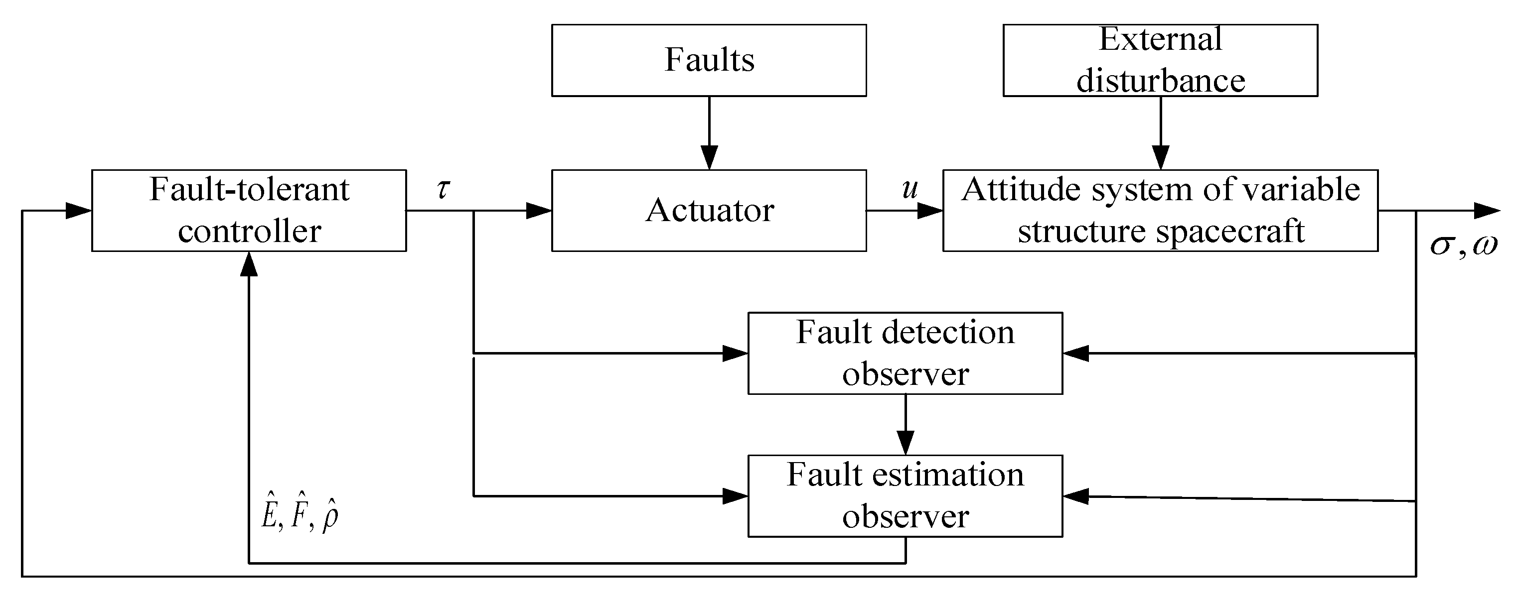
Compared with existing state-of-the-art detectors [30,31], the proposed detector considers complete failure and variable structure conditions, and is more suitable for dexterous spacecraft. It is seen from Figure 1 that the output signal of attitude controller τ and the angular velocity ω are measured by the gyro as the inputs of the fault detection and estimation observer and the estimated angular velocity is the output of the fault detection and estimation observer. In addition, the estimated parameter values which can be obtained using the designed adaptive updated algorithms (35) and (38), were also used in the design of the fault estimation observer.

4. Fault-Tolerant Controller Design

4.1. Active FTC without Actuator Saturation

In this section, an active FTC strategy is proposed for the faulty attitude systems (1) and (11) without actuator saturation. First, a fast terminal sliding model surface is designed as

$$S=\omega +(k_1+k_{h,1}(J_{VS}))\sigma +k_2\mathrm{sig}{(\sigma )}^{p/(q+h(J_{VS}))}$$

(53)

where S = [S₁, S₂, S₃]^T ∈ R³ is the sliding mode variable; k₁ > 0, k₂ > 0 are two positive scalars; k_h,1(J_VS), h(J_VS) are the variable structure harmonic functions with J_VS as the argument, which are all known scalars, and 0 < (p/(q + h(J_VS))) < 1; and p, q are positive odd integers. The function sig(σ)p/(q + h(J_VS)) is defined as

$$\mathrm{sig}{(\sigma )}^{p/(q+h(J_{VS}))}=\left[\begin{array}{c}{\left|\varphi \right|}^{p/(q+h(J_{VS}))}\mathrm{sign}(\varphi )\\ {\left|\theta \right|}^{p/(q+h(J_{VS}))}\mathrm{sign}(\theta )\\ {\left|\psi \right|}^{p/(q+h(J_{VS}))}\mathrm{sign}(\psi )\end{array}\right]$$

(54)

Taking the derivative of sliding variable S with respect to time yields

$$\dot{S}=\dot{\omega }+(k_1+k_{h,1}(J_{VS}))\dot{\sigma }+\frac{k_{2}p}{q+h(J_{VS})}\mathrm{diag}({\left|\sigma \right|}^{[p/(q+h(J_{VS}))]-1})\dot{\sigma }$$

(55)

It was noted that Equation (55) contains a negative fractional term [p/(q + h(J_VS))]⁻¹, the singularity occurs while σ_j = 0 and its derivative is nonzero. To avoid the singularity problem, the derivative of S is modified as

$$\dot{S}=\dot{\omega }+(k_1+k_{h,1}(J_{VS}))\dot{\sigma }+k_2{S}^{*}(\sigma )$$

(56)

where

$$S^{*}(\sigma )={[S_1^{*}(\sigma ), S_2^{*}(\sigma ), S_3^{*}(\sigma )]}^T\in R^{3\times 1}$$

(57)

with

$$S_i^{*}(\sigma )=\{\begin{array}{c}\frac{p}{q+h(J_{VS})}{\left|{\sigma }_i\right|}^{[p/(q+h(J_{VS}))]-1}{\dot{\sigma }}_i, if {\dot{\sigma }}_i\ne 0, \left|{\sigma }_i\right|\ge \epsilon \\ \frac{p}{q+h(J_{VS})}{\left|\epsilon \right|}^{[p/(q+h(J_{VS}))]-1}{\dot{\sigma }}_i, if {\dot{\sigma }}_i\ne 0, \left|{\sigma }_i\right|<\epsilon \\ 0, if {\dot{\sigma }}_i=0\end{array}$$

(58)

where S_i*(σ) is the ith component of S*(σ) and ε is a small positive constant.

Substituting Equation (11) into Equation (56), it is easily known that

$$\begin{array}{l}\dot{S}=-{(J+J_{VS})}^{-1}\Lambda (J+J_{VS})\omega +{(J+J_{VS})}^{-1}DE\tau +(J\\ +J_{VS}{)}^{-1}DF+\rho (t)+(k_1+k_{h,1}(J_{VS}))\dot{\sigma }+k_2{S}^{*}(\sigma )\end{array}$$

(59)

According to the sliding mode control idea, sliding mode dynamics need to match a reaching law. This study selected an improved exponential reaching law as

$$\dot{S}=-({\upsilon }_1+{\upsilon }_{h,1}^{}(J_{VS}))S-({\upsilon }_2+{\upsilon }_{h,2}(J_{VS}\left)\right)\mathrm{sig}{(S)}^{p/(q+h(J_{VS}))}$$

(60)

where

$$\{\begin{array}{l}{\upsilon }_1=\mathrm{diag}\{{\upsilon }_{11}, {\upsilon }_{12}, {\upsilon }_{13}\}>0\\ {\upsilon }_2=\mathrm{diag}\{{\upsilon }_{21}, {\upsilon }_{22}, {\upsilon }_{23}\}>0\end{array}$$

(61)

$$\{\begin{array}{l}{\upsilon }_{h,1}(J_{VS})=\mathrm{diag}\{{\upsilon }_{h,11}, {\upsilon }_{h,12}, {\upsilon }_{h,13}\}>0\\ {\upsilon }_{h,2}(J_{VS})=\mathrm{diag}\{{\upsilon }_{h,21}, {\upsilon }_{h,22}, {\upsilon }_{h,23}\}>0\end{array}$$

(62)

Equations (61) and (62) are the diagonal matrices. υ_h,11, υ_h,12, υ_h,13, υ_h,21, υ_h,22, and υ_h,23 are the known harmonic functions with J_VS as the argument. To derive the FTC scheme of this paper, an assumption is introduced in this position.

Assumption 4.

There exists two unknown constants γ ≥ 0 and δ ≥ 0, such that the following inequalities are satisfied

$$\Vert -{(J+J_{VS})}^{-1}\Lambda (J+J_{VS})\omega \Vert \le \gamma$$

(63)

$$\Vert (k_1+k_{h,1}(J_{VS}))\dot{\sigma }+k_2{S}^{*}(\sigma )\Vert \le \delta \Vert \dot{\sigma }\Vert$$

(64)

In the following, the third result of this study is given in the form of Theorem 3.

Theorem 3.

Considering the faulty attitude systems (1) and (11) of a flexible variable structure spacecraft without actuator saturation, a fast terminal sliding mode-based active FTC scheme is given by

$$\tau =-{\widehat{E}}^2{D}^T{[{(J+J_{VS})}^{-1}D{\widehat{E}}^3{D}^T]}^{-1}({\tau }_1+{\tau }_2)$$

(65)

with

$${\tau }_1=({\upsilon }_1+{\upsilon }_{h,1}(J_{VS}))S+({\upsilon }_2+{\upsilon }_{h,2}(J_{VS}))\mathrm{sig}{(S)}^{p/(q+h(J_{VS}))}$$

(66)

$${\tau }_2=\frac{S}{\Vert S\Vert +\varsigma }(\widehat{\delta }\Vert \dot{\sigma }\Vert +\widehat{\gamma }+\Vert {(J+J_{VS})}^{-1}D\widehat{F}\Vert +\Vert {\widehat{W}}^T\phi (t)+{\widehat{\epsilon }}_0\Vert )$$

(67)

$$\dot{\widehat{\gamma }}=(c_4+c_{h,4}(J_{VS}))\Vert S\Vert$$

(68)

$$\dot{\widehat{\delta }}=(c_5+c_{h,5}(J_{VS}))\Vert S\Vert \Vert \dot{\sigma }\Vert$$

(69)

where ς > 0 is a small positive scalar, c_i > 0(i = 4, 5) are positive scalars, and c_h,i are the variable structure harmonic functions; additionally, these parameters can be preset. Then, the state trajectory of the faulty attitude systems can converge to a neighborhood of the origin in finite time.

Proof of Theorem 3.

Let

$$\{\begin{array}{l}\tilde{\delta }=\widehat{\delta }-\delta \\ \tilde{\gamma }=\widehat{\gamma }-\gamma \end{array}$$

(70)

a Lyapunov candidate function was selected as

$$V_3=\frac{1}{2}{S}^{T}S+\frac{1}{2(c_4+c_{h,4}(J_{VS}))}{\tilde{\gamma }}^2+\frac{1}{2(c_5+c_{h,5}(J_{VS}))}{\tilde{\delta }}^2+V_2$$

(71)

Taking the derivative of V₃ along the trajectory of Equation (59) yields

$$\begin{array}{l}{\dot{V}}_3=S^T[-{(J+J_{VS})}^{-1}\Lambda (J+J_{VS})\omega +{(J+J_{VS})}^{-1}DE\tau +(J\\ +J_{VS}{)}^{-1}DF+\rho (t)+(k_1+k_{h,1}(J_{VS}))\dot{\sigma }+k_2{S}^{*}(\sigma )]+\frac{\tilde{\gamma }\dot{\widehat{\gamma }}}{C_{4,JVS}}\\ +\frac{\tilde{\delta }\dot{\widehat{\delta }}}{C_{5,JVS}}+{\dot{V}}_2\end{array}$$

(72)

where

$$\{\begin{array}{l}{C}_{4,JVS}=c_4+c_{h,4}(J_{VS})\\ C_{5,JVS}=c_5+c_{h,5}(J_{VS})\end{array}$$

(73)

Substituting Equation (59) into the above equation, it can be seen that

$$\begin{array}{l}{\dot{V}}_3\le \Vert S\Vert (\Vert (k_1+k_{h,1}(J_{VS}))\dot{\sigma }+k_2{S}^{*}(\sigma )\Vert -\widehat{\delta }\Vert \dot{\sigma }\Vert )+\tilde{\gamma }\Vert S\Vert +\tilde{\delta }\Vert S\Vert \Vert \dot{\sigma }\Vert \\ +\Vert S\Vert (\Vert -{(J+J_{VS})}^{-1}\Lambda (J+J_{VS})\omega \Vert -\widehat{\gamma })+S^T[-({\upsilon }_1+{\upsilon }_{h,1}(J_{VS}))S\\ -({\upsilon }_2+{\upsilon }_{h,2}(J_{VS}\left)\right)\mathrm{sig}{(S)}^{p/(q+h(J_{VS}))}]-\alpha V_2+\beta \\ \le S^T[-({\upsilon }_1+{\upsilon }_{h,1}(J_{VS}))S-({\upsilon }_2+{\upsilon }_{h,2}(J_{VS}\left)\right)\mathrm{sig}{(S)}^{p/(q+h(J_{VS}))}]+\beta \\ \le -S^T({\upsilon }_1+{\upsilon }_{h,1}(J_{VS}))S-2^{\{[p/(q+h(J_{VS}))]+1\}/2}[\frac{1}{2}{S}^T({\upsilon }_2\\ +{\upsilon }_{h,2}(J_{VS}\left)\right)S{]}^{\{[p/(q+h(J_{VS}))]+1\}/2}+\beta \\ \le -2{\lambda }_{\min }({\upsilon }_1+{\upsilon }_{h,1}(J_{VS}))(1-\frac{\Omega }{V_3})V_3-2^{\{[p/(q+h(J_{VS}))]+1\}/2}{\lambda }_{\min }({\upsilon }_2\\ +{\upsilon }_{h,2}\left(J_{VS}\right))(1-{(\frac{\Omega }{V_3})}^{\{[p/(q+h(J_{VS}))]+1\}/2})V_3^{\{[p/(q+h(J_{VS}))]+1\}/2}+\beta \end{array}$$

(74)

where

$$\Omega =(1/2C_{4,JVS}){\tilde{\gamma }}^2(t)+(1/2C_{5,JVS}){\tilde{\delta }}^2(t)+V_2$$

(75)

and

$$\{\begin{array}{l}(\Omega /V_3)<1\\ {(\Omega /V_3)}^{\{[p/(q+h(J_{VS}))]+1\}/2}<1\end{array}$$

(76)

Define

$${\vartheta }_1=2{\lambda }_{\min }({\upsilon }_1+{\upsilon }_{h,1}(J_{VS}))(1-(\Omega /V_3))$$

(77)

$${\vartheta }_2=2^{\{[p/(q+h(J_{VS}))]+1\}/2}{\lambda }_{\min }({\upsilon }_2+{\upsilon }_{h,2}(J_{VS}))[1-{(\Omega /V_3)}^{\{[p/(q+h(J_{VS}))]+1\}/2}]$$

(78)

then, we have

$${\dot{V}}_3\le -{\vartheta }_1{V}_3-{\vartheta }_2{V}_3^{\{[p/(q+h(J_{VS}))]+1\}/2}+\beta$$

(79)

If V₃ > β/ϑ₁, the inequality (79) is further rewritten as

$${\dot{V}}_3\le -({\vartheta }_1-\beta /V_3)V_3-{\vartheta }_2{V}_3^{\{[p/(q+h(J_{VS}))]+1\}/2}$$

(80)

According to Lemma 1, the convergence time satisfies the following inequality

$$T_S\le t_0+\frac{1}{({\vartheta }_1-\beta /V_3)(1-\frac{p}{q+h(J_{VS})})}\ln \{\frac{({\vartheta }_1-\beta /V_3)V_3{(t_0)}^{[1-p/(q+h(J_{VS}))]/2}}{{\vartheta }_2}+1\}$$

(81)

where t₀ is the initial time and V₃(t₀) is the initial value.

If $V_3^{\{[p/(q+h(J_{VS}))]+1\}/2}>\beta /{\vartheta }_2$, the inequality (79) is rewritten in the following form

$${\dot{V}}_3\le -{\vartheta }_1{V}_3-({\vartheta }_2-\beta /V_3^{\{[p/(q+h(J_{VS}))]+1\}/2})V_3^{\{[p/(q+h(J_{VS}))]+1\}/2}$$

(82)

Similarly, the convergence time satisfies

$$T_S\le t_0+\frac{1}{{\vartheta }_1(1-\frac{p}{q+h(J_{VS})})}\ln \left\{\frac{{\vartheta }_1{V}_3{(t_0)}^{[1-p/(q+h(J_{VS}))]/2}}{{\vartheta }_2-\beta /V_3^{\{[p/(q+h(J_{VS}))]+1\}/2}}+1\right\}$$

(83)

Therefore, the state trajectory of the faulty closed-loop attitude systems can converge into a neighborhood of the origin in finite time. This completes the proof. □

Remark 4.

In the study by [29], a non-singular terminal sliding model surface was designed as:

$$S=\omega +k{\mathrm{sig}}^{(a/b)}(\sigma ),$$

where k > 0 and 1 < (a/b) < 2. It provides a fast convergence rate at a distance from the origin and becomes slow as it nears the equilibrium. The closer to the origin, the slower the convergence rate. In this paper, a non-singular fast terminal sliding model surface was designed in the form:

$$S=\omega +(k_1+k_{h,1}(J_{VS}))\sigma +k_2\mathrm{sig}{(\sigma )}^{p/(q+h(J_{VS}))},$$

when the system states are far away from zero, the linear term k₁σ offers a fast convergence rate, and when the system states are close to zero, the nonlinear term k₂sig(σ)^p/(q+h(JVS)) guarantees the finite-time convergence. Therefore, the system states converge quickly to the sliding model surface designed in this study.

4.2. Active Anti-Saturation FTC

To address the problem of actuator saturation, the other active FTC scheme is further presented in this section. Consider the dynamics Equation (7) of a flexible variable structure spacecraft under actuator saturation, which is described by

$$\dot{\omega }=-{(J+J_{VS})}^{-1}\Lambda (J+J_{VS})\omega +{(J+J_{VS})}^{-1}D\mathrm{sat}(\tau )+\rho (t)$$

(84)

in which sat(τ) is given by

$$\mathrm{sat}({\tau }_i)=\{\begin{array}{ll}{\tau }_i,& if \left|{\tau }_i\right|<{\tau }_{\max }\hfill \\ {\tau }_{\max }\mathrm{sign}({\tau }_i),& otherwise\end{array}$$

(85)

where t is the designed control input and t_max is the upper boundary of saturation nonlinearity.

Here, a nonlinear saturation function is introduced to handle the saturation input

$$\mathrm{sat}(\tau )=\chi (\tau )\tau$$

(86)

where χ(τ) = diag{χ₁(τ₁), …, χ_n(τ_n)} represents the saturation characteristic of the actuators with

$${\chi }_i({\tau }_i)=\{\begin{array}{ll}1,& if \left|{\tau }_i\right|\le {\tau }_{\max }\\ \frac{{\tau }_{\max }}{{\tau }_i}\mathrm{sign}({\tau }_i),& otherwise\end{array}$$

(87)

It was assumed that χ_i(τ_i) satisfies the following constraint

$$0<\mu \le \min ({\chi }_i({\tau }_i))\le 1$$

(88)

By referring to the fault modeling method developed in the study by [21], the faulty dynamics equation in the actuator saturation case is written as

$$\begin{array}{l}\dot{\omega }=-{(J+J_{VS})}^{-1}\Lambda (J+J_{VS})\omega +{(J+J_{VS})}^{-1}D(E\mathrm{sat}(\tau )\\ +F)+\rho (t)\end{array}$$

(89)

By designing the same fast terminal sliding model surface

$$S=\omega +(k_1+k_{h,1}(J_{VS}))\sigma +k_2\mathrm{sig}{(\sigma )}^{p/(q+h(J_{VS}))}$$

(90)

the derivative of S is given by

$$\begin{array}{l}\dot{S}=-{(J+J_{VS})}^{-1}\Lambda (J+J_{VS})\omega +{(J+J_{VS})}^{-1}D(E\mathrm{sat}(\tau )+F)\\ +\rho (t)+(k_1+k_{h,1}(J_{VS}))\dot{\sigma }+k_2{S}^{*}(\sigma )\end{array}$$

(91)

Based on the above content, the fourth result of this study is given in the form of Theorem 4.

Theorem 4.

Considering the faulty attitude systems (1) and (89) in the actuator saturation case, a fast terminal sliding model-based active FTC scheme is designed as

$$\tau =-{\widehat{E}}^2{D}^T{[{(J+J_{VS})}^{-1}D{\widehat{E}}^3{D}^T]}^{-1}({\tau }_1+{\tau }_2)$$

(92)

with

$${\tau }_1=({\upsilon }_1+{\upsilon }_{h,1}(J_{VS}))S+({\upsilon }_2+{\upsilon }_{h,2}(J_{VS}\left)\right)\mathrm{sig}{(S)}^{p/(q+h(J_{VS}))}$$

(93)

$${\tau }_2=\frac{S}{\Vert S\Vert +\varsigma }\widehat{\mu }[\widehat{\gamma }+\widehat{\delta }\Vert \dot{\sigma }\Vert +\Vert {(J+J_{VS})}^{-1}D\widehat{F}\Vert +\Vert {\widehat{W}}^T\phi (t)+{\widehat{\epsilon }}_0\Vert ]$$

(94)

The adaptive parameter updated algorithms are given by

$$\dot{\widehat{\gamma }}=(c_6+c_{h,6}(J_{VS}))\Vert S\Vert$$

(95)

$$\dot{\widehat{\delta }}=(c_7+c_{h,7}(J_{VS}))\Vert S\Vert \Vert \dot{\sigma }\Vert$$

(96)

$$\begin{array}{l}\dot{\widehat{\mu }}=(c_8+c_{h,8}(J_{VS})){\widehat{\mu }}^3\Vert S\Vert (\widehat{\gamma }+\widehat{\delta }\Vert \dot{\sigma }\Vert +\Vert {(J+J_{VS})}^{-1}D\widehat{F}\Vert \\ +\Vert {\widehat{W}}^T\phi (t)+{\widehat{\epsilon }}_0\Vert )\end{array}$$

(97)

where ς > 0 is a small positive constant, c_i > 0 (i = 6, 7, 8) are positive scalars, and c_h,i are the variable structure harmonic functions, all of which can be preset. Then, the state trajectory of the faulty attitude systems can converge in finite time.

Proof of Theorem 4.

Defining

$$\tilde{\mu }={\widehat{\mu }}^{-1}-\mu$$

(98)

a Lyapunov candidate function was selected as

$$\begin{array}{l}{V}_4=\frac{1}{2}{S}^{T}S+\frac{1}{2(c_6+c_{h,6}(J_{VS}))}{\tilde{\gamma }}^2+\frac{1}{2(c_7+c_{h,7}(J_{VS}))}{\tilde{\delta }}^2\\ +\frac{1}{2(c_8+c_{h,8}(J_{VS}))}{\tilde{\mu }}^2+V_2\end{array}$$

(99)

Set

$$\{\begin{array}{l}{C}_{6,JVS}=c_6+c_{h,6}(J_{VS})\\ C_{7,JVS}=c_7+c_{h,7}(J_{VS})\\ C_{8,JVS}=c_8+c_{h,8}(J_{VS})\end{array}$$

(100)

and taking the derivative of V₄ along the trajectory of Equation (91) yields

$$\begin{array}{l}{\dot{V}}_4=S^T[-{(J+J_{VS})}^{-1}\Lambda (J+J_{VS})\omega +{(J+J_{VS})}^{-1}DE\mathrm{sat}(\tau )\\ +{(J+J_{VS})}^{-1}DF+\rho (t)+(k_1+k_{h,1}(J_{VS}))\dot{\sigma }+k_2{S}^{*}(\sigma )]\\ +\frac{\tilde{\gamma }\dot{\widehat{\gamma }}}{C_{6,JVS}}+\frac{\tilde{\delta }\dot{\widehat{\delta }}}{C_{7,JVS}}-\frac{\tilde{\mu }{\widehat{\mu }}^{-2}\dot{\widehat{\mu }}}{C_{8,JVS}}+{\dot{V}}_2\end{array}$$

(101)

Substituting Equation (92) into ${\dot{V}}_4$, it is easily known that

$$\begin{array}{l}{\dot{V}}_4\le \Vert S\Vert [\Vert -{(J+J_{VS})}^{-1}\Lambda (J+J_{VS})\omega \Vert -\widehat{\gamma }-\widehat{\delta }\Vert \dot{\sigma }\Vert \\ -\Vert {(J+J_{VS})}^{-1}D\widehat{F}\Vert -\Vert {\widehat{W}}^T\phi (t)+{\widehat{\epsilon }}_0\Vert +\Vert {(J+J_{VS})}^{-1}DF\Vert +\Vert \rho (t)\Vert \\ +\Vert (k_1+k_{h,1}(J_{VS}))\dot{\sigma }+k_2{S}^{*}(\sigma )\Vert +\tilde{\gamma }\Vert S\Vert +\tilde{\delta }\Vert S\Vert \Vert \dot{\sigma }\Vert +\mu S^T[-({\upsilon }_1\\ +{\upsilon }_{h,1}(J_{VS}))S-({\upsilon }_2+{\upsilon }_{h,2}(J_{VS}))\mathrm{sig}{(S)}^{p/(q+h(J_{VS}))}]+{\dot{V}}_2\\ \le \Vert S\Vert [(\Vert -{(J+J_{VS})}^{-1}\Lambda (J+J_{VS})\omega \Vert -\gamma )+(\Vert \rho (t)\Vert -\Vert {\widehat{W}}^T\phi (t)+{\widehat{\epsilon }}_0\Vert )\\ +(\Vert (k_1+k_{h,1}(J_{VS}))(J+J_{VS})\dot{\sigma }+k_2(J+J_{VS})S^{*}(\sigma )\Vert -\delta \Vert \dot{\sigma }\Vert )\\ +(\Vert {(J+J_{VS})}^{-1}DF\Vert -\Vert {(J+J_{VS})}^{-1}D\widehat{F}\Vert )]+\mu S^T[-({\upsilon }_1+{\upsilon }_{h,1}(J_{VS}))S\\ -({\upsilon }_2+{\upsilon }_{h,2}(J_{VS}))\mathrm{sig}{(S)}^{p/(q+h(J_{VS}))}]-\alpha V_2+\beta \\ \le \mu S^T[-({\upsilon }_1+{\upsilon }_{h,1}(J_{VS}))S-({\upsilon }_2+{\upsilon }_{h,2}(J_{VS}))\mathrm{sig}{(S)}^{p/(q+h(J_{VS}))}]+\beta \\ \le -2\mu [\frac{1}{2}{S}^T({\upsilon }_1+{\upsilon }_{h,1}(J_{VS}))S]-2^{\{[p/(q+h(J_{VS}))]+1\}/2}\mu [\frac{1}{2}{S}^T({\upsilon }_2\\ +{\upsilon }_{h,2}(J_{VS}))S{]}^{\{[p/(q+h(J_{VS}))]+1\}/2}+\beta \\ \le -2\mu {\lambda }_{\min }({\upsilon }_1+{\upsilon }_{h,1}(J_{VS}))(1-\frac{\Theta }{V_4})V_4-2^{\{[p/(q+h(J_{VS}))]+1\}/2}\mu {\lambda }_{\min }({\upsilon }_2\\ +{\upsilon }_{h,2}(J_{VS}))(1-{(\frac{\Theta }{V_4})}^{\{[p/(q+h(J_{VS}))]+1\}/2})V_4^{\{[p/(q+h(J_{VS}))]+1\}/2}+\beta \end{array}$$

(102)

where

$$\Theta =\frac{1}{2C_{6,JVS}}{\tilde{\gamma }}^2(t)+\frac{1}{2C_{7,JVS}}{\tilde{\delta }}^2(t)+\frac{1}{2C_{8,JVS}}{\tilde{\mu }}^2(t)+V_2$$

(103)

and

$$\{\begin{array}{l}\frac{\Theta }{V_4}<1\\ {(\frac{\Theta }{V_4})}^{\{[p/(q+h(J_{VS}))]+1\}/2}<1\end{array}$$

(104)

Define

$${\vartheta }_3=2\mu {\lambda }_{\min }({\upsilon }_1+{\upsilon }_{h,1}(J_{VS}))(1-(\frac{\Theta }{V_4}))$$

(105)

$${\vartheta }_4=2^{\{[p/(q+h(J_{VS}))]+1\}/2}\mu {\lambda }_{\min }({\upsilon }_2+{\upsilon }_{h,2}(J_{VS}))(1-{(\frac{\Theta }{V_4})}^{\{[p/(q+h(J_{VS}))]+1\}/2})$$

(106)

then, we have

$${\dot{V}}_4\le -{\vartheta }_3{V}_4-{\vartheta }_4{V}_4^{\{[p/(q+h(J_{VS}))]+1\}/2}+\beta$$

(107)

By referring to the proof process of Theorem 3, all the state trajectory of the considered closed-loop attitude systems can converge to a neighborhood of the origin in finite time. This completes the proof. The unknown P₁ and P₂ could be obtained by solving (23) and (45) using the linear matrix inequality toolbox in MATLAB. Hence, the fault detection threshold J_th and the adaptive fault parameter updated algorithms could be accomplished online and the final FTC (64) or (91) was successfully reconstructed to the faulty attitude systems. The whole active FTC scheme in this study had an acceptable computational burden and could be easily applied. □

Remark 5.

In this study, the variable structure control has one more J_VS including the harmonic functions with J_VS as the independent variable than the non-variable structure control. When J_VS = 0, the harmonic functions in the controller are 0. This shows that the control method without the variable structure is the same as the control method after all harmonic functions are removed. In NASA’s 1979 technical report ‘Simulator study of stall/poststall characteristics of a fighter airplane with relaxed longitudinal static stability’, the mechanical structure of the aircraft in the angular rate channel is represented by the inertia coefficient, and the active variable structure causes the inertia coefficient to change. That is, nine incremental functions are added after the reported c₁–c₉. The flexible variable structure parameter J_VS in this paper is this incremental function, and its physical meaning is completely consistent.

5. Simulation

In this section, we use the Links-Box semi-physical simulator to verify the effectiveness of algorithms. Links-Box automatically converts the MATLAB simulation models to the embedded control prototype and support engineering hardware to test in the models. The physical device can be directly connected to the rapid prototyping simulator to dynamically verify controller performance. The features of software package Links-RT are: (1) adapting to the models built in MATLAB; (2) providing input and output hardware to enable users to integrate the hardware environment into the simulation models; (3) automatic conversion of MATLAB model codes to VxWorks codes; (4) providing communication, storage, scheduling, and other services in VxWorks.

To illustrate our adaptive method and evaluate its effectiveness, we applied it to an attitude system of a variable structure spacecraft where the physical parameters were set according to [32]. The fixed structure inertia J, variable structure parameter J_VS, and actuator distribution matrix are given by

$$\begin{gathered} J=\left[\begin{array}{ccc}40& 12& 9\\ 12& 90& 14\\ 9& 14& 40\end{array}\right]\hspace{0.17em}\mathrm{kg}\cdot {\mathrm{m}}^3, D=\left[\begin{array}{cccc}1& 0& 0& \frac{1}{\sqrt{3}}\\ 0& 1& 0& \frac{1}{\sqrt{3}}\\ 0& 0& 1& \frac{1}{\sqrt{3}}\end{array}\right], \\ {J}_{VS}=\{\begin{array}{l}\left[\begin{array}{ccc}10\tanh [10(t-20)]& 0& 5\tanh [10(t-20)]\\ 0& 7\tanh [10(t-20)]& 0\\ 3\tanh [10(t-20)]& 0& 5\tanh [10(t-20)]\end{array}\right]\hspace{0.17em}\mathrm{kg}\cdot {\mathrm{m}}^3, t\ge 20\hspace{0.17em}\mathrm{s}\\ 0, 0\le t<20\hspace{0.17em}\mathrm{s}\end{array} \end{gathered}$$

where tanh(·) is the hyperbolic tangent function which satisfies:

$$\tanh [10(t-20)]=\frac{e^{10(t-20)}-e^{-10(t-20)}}{e^{10(t-20)}+e^{-10(t-20)}}$$

The inertia uncertainty was chosen as ΔJ = 2diag{sin(0.1t), 2cos(0.2t), sin(0.1t)} kg·m³, and the external disturbance vector was chosen as d(t) = [0.1sin(0.1t), 0.2sin(0.2t), 0.1sin(0.3t)] N·m. The initial attitude angles were chosen as σ₀ = [0.5, 0.3, −0.5]^T deg, and the initial angular velocities were selected as ω₀ = [0.5, 0.3, −0.6]^T deg/s. The gyro was used for the angular velocity measurement, and it will inevitably encounter measurement noise in practical applications. The output signal of each gyro could be modeled as

$${\omega }_g(t)=\omega (t)+{\omega }_n(t)$$

(108)

where ω_g(t) is the actual measured angular velocity, ω_n(t) is the zero mean Gaussian white noise process, and the covariance of ω_n(t) is given by

$$E\{{\omega }_n(t){\omega }_n^T(h)\}=I_3{\eta }_n^2\alpha (t-h)$$

(109)

where α(t − h) is the Dirac delta function [21]. All the variable structure harmonic functions are linear functions.

It was set that there are four reaction wheels used for the attitude control of a variable structure spacecraft. The actuator saturation is addressed in the position, namely, the maximum torque of each actuator was constrained to be the value of 0.8 N·m. The first reaction wheel works normally, the second reaction wheel decreases 40% of the control effectiveness after t = 2 s, the third reaction wheel occurs a bias fault f₃ = 0.4 N·m after t = 2 s, and the fourth reaction wheel occurs a complete failure fault after t = 2 s.

In the design of the fault detection observer, the positive matrix A₁ was chosen as diag{2, 6, 2}, and the unknown positive matrix P₁ could be solved from Equation (23) as diag{20, 10, 20}. In the design of the fault estimation observer, the Hurwitz matrix A₂ was chosen as diag{−3, −6, −5}, and the unknown positive matrix P₂ could be solved from inequality (45) as diag{19, 21, 6}. In addition, the other constant parameters were selected as c₀ = 0.9, c₁ = 0.8, c₂ = 0.7, c₃ = 0.9, and $\widehat{W}(0)=\mathrm{diag}\{1, 1, 1\}$. The parameters of the FTC controller (92) were selected as follows: k₁ = 0.25, k₂ = 0.11, p = 4, q = 7, υ₁ = diag{1.9, 2.5, 4.5}, υ₂ = diag{3.6, 4.8, 1.5}, ς = 0.03, c₆ = 1.5, c₇ = 1.4, and c₈ = 1.4.

Figure 2 shows the evolution of residual evaluation function ǀǀrǀǀ_2,T, in which the dashed line represents the fault threshold, and the solid line represents the fault detector residual norm. It can be seen that once the actuator faults happened, the designed residual exceeded the threshold J_th at t = 2 s, which could trigger the fault estimation observer to start working.

At t = 20 s, the system entered the variable structure mode, and Figure 2b shows that as long as no fault occurs, the residual never exceeds J_th, and therefore, the proposed fault detector could adapt to the variable structure mode.

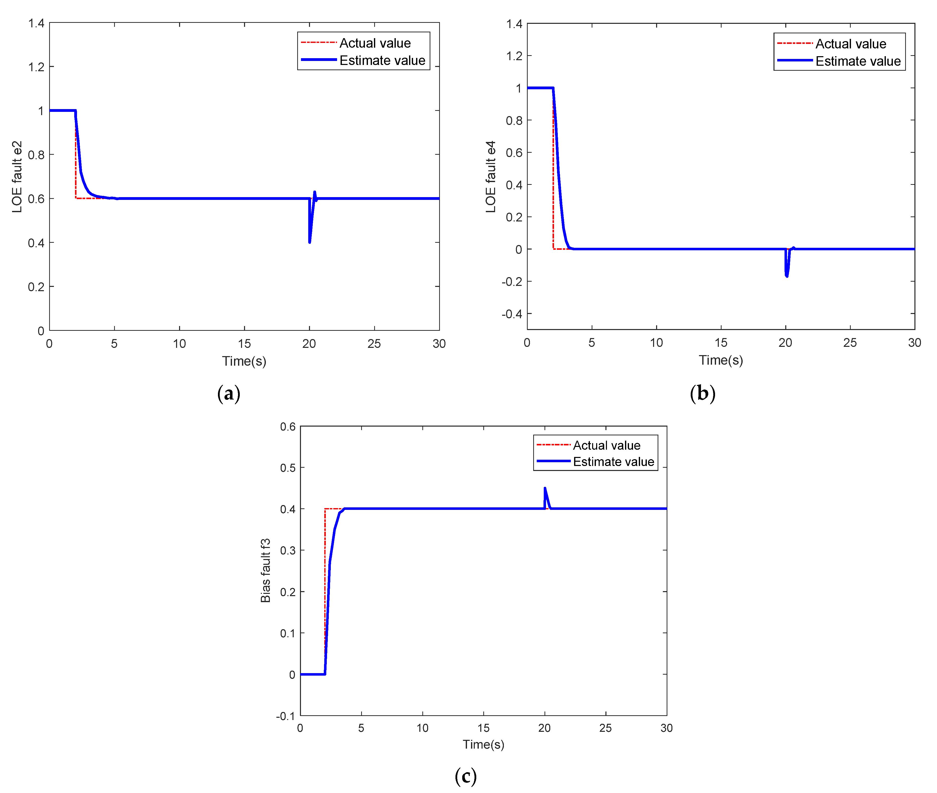
Figure 3 is the corresponding fault estimation result, and the three different types of actuator faults could be estimated accurately using the fault estimation observer (33) and the adaptive estimation algorithms (35)–(38).

For the purpose of comparison, the passive non-singular terminal sliding mode-based FTC scheme designed in [32] and the FTC scheme designed in this article are adopted to simulate the same faulty attitude systems in this section. When the considered actuator fault occurs, the corresponding semi-physical simulation results (including the attitude angle σ, and the angular velocity ω) using the proposed FTC scheme are depicted in Figure 4, and it is seen from Figure 4 that the simulation results using the proposed FTC scheme developed in this paper had fast and accurate tracking performance. The comparison with the scheme of [32] is in

Table 2. Comparative analysis of performance with the prior art in [32].

FTC Scheme	Convergence Time: σ	Steady Precision: σ	Convergence Time: ω	Steady Precision: ω
FTC in [30]	—	2	—	1.5
FTC in this paper	5.1	4 × 10−5	5.2	6 × 10−5

, which shows that the passive non-singular terminal sliding mode-based FTC scheme could not make the output converge, and the scheme of this study had obvious advantages.

The biggest difficulty of this study was to take into account the nominal mode and the variable structure mode. Because of the uncertainty brought by the variable structure, this study designed many harmonic functions that were nearly twice as much as the nominal control to solve this problem. Finally, the effect of overshoot was limited and the final parameter setting was successful.

To further emphasize the superiority of the proposed method, the control performance comparisons using three different FTC schemes are also given in Table 2,

Table 3. Comparative analysis of performance with proposed FTC without fault estimation.

FTC Scheme	Convergence Time: σ	Steady Precision: σ	Convergence Time: ω	Steady Precision: ω
Passive FTC without fault estimation	—	0.73	—	0.52
FTC in this paper	5.1	4 × 10−5	5.2	6 × 10−5

,

Table 4. Comparative analysis of performance with proposed FTC without variable structure harmonic functions.

FTC Scheme	Convergence Time: σ	Steady Precision: σ	Convergence Time: ω	Steady Precision: ω
FTC without variable structure method	—	∞	—	∞
FTC in this paper	5.1	4 × 10−5	5.2	6 × 10−5

and

Table 5. Comparative analysis of performance with proposed FTC without anti-saturation method.

FTC Scheme	Convergence Time: σ	Steady Precision: σ	Convergence Time: ω	Steady Precision: ω
FTC without anti-saturation method	34.5	2 × 10−4	35.7	4.5 × 10−4
FTC in this paper	5.1	4 × 10−5	5.2	6 × 10−5

. Where “—” indicates that the curve does not converge and therefore has no convergence time, “∞” indicates that the curve diverges and thus the maximum steady precision tends to infinity as time increases.

If the method of this paper removes the variable structure harmonic functions, the tracking curves diverge. If the method of this paper does not have an anti-saturation scheme, i.e., only uses Algorithm (65), the maximum convergence time increases by a factor of seven. If the method of this paper does not have a fault estimation scheme (passive FTC of Table 3), the static errors of the tracking curves are still more than 5% of the expected outputs. As can be seen, none of the above three comparison schemes can meet the demand. Our improved adaptive FTC scheme with fast terminal sliding mode and variable structure harmonic functions could achieve higher attitude tracking accuracy and faster convergence rate than [32], the proposed FTC without variable structure method, and the proposed FTC without anti-saturation method.

6. Conclusions

In this paper, an improved FTC scheme was developed for the attitude systems of a flexible variable structure spacecraft in the presence of disturbances, multiple actuator faults, and saturation. A fault detection and estimation approach is presented to detect the time of actuator faults occurrence and estimate the amplitude of unknown faults. On this basis, the improved adaptive FTC with variable structure harmonic functions was designed in the framework of the fast terminal sliding mode technique, which ensures that the faulty attitude system is asymptotical convergence in finite time. Thus, the proposed FTC scheme achieves unified compensation for multi-location (different actuator channels) multi-type (bias and complete failures) concurrent faults in nominal and variable structure flight modes. Simulation results verified the good fault-tolerant performance using the proposed active FTC scheme. However, the proposed FTC scheme did not consider the sensor fault problem, and how to design a FTC strategy to compensate the effects of sensor fault is our future research works.

References

- Thongchom, C.; Roodgar, S.P.; Roudgar, S.P.; Refahati, N.; Sirimontree, S.; Keawsawasvong, S.; Titotto, S. Dynamic response of fluid-conveying hybrid smart carbon nanotubes considering slip boundary conditions under a moving nanoparticle. Mech. Adv. Mater. Struct. 2022, 7, 1–4. [Google Scholar] [CrossRef]
- Thongchom, C.; Saffari, P.R.; Refahati, N.; Saffari, P.R.; Pourbashash, H.; Sirimontree, S.; Keawsawasvong, S. An analytical study of sound transmission loss of functionally graded sandwich cylindrical nanoshell integrated with piezoelectric layers. Sci. Rep. 2022, 12, 1–16. [Google Scholar] [CrossRef] [PubMed]
- Hang, B.; Cao, S.; Fang, Y. Adaptive anti-disturbance fault tolerant control of flexible satellites with input saturation. In Advances in Guidance, Navigation and Control; Yan, L., Duan, H., Yu, X., Eds.; Springer: Singapore, 2022; Volume 644, pp. 1277–1287. [Google Scholar]
- Ashayeri, L.; Doustmohammadi, A.; Saberi, F.F. Fault-tolerant control allocation of a flexible satellite with an infinite- dimensional model. Proc. Inst. Mech. Eng. Part G J. Aerosp. Eng. 2021, 235, 2069–2080. [Google Scholar] [CrossRef]
- Liu, C.; Vukovich, G.; Sun, Z.; Shi, K. Observer-based fault-tolerant attitude control for spacecraft with input delay. J. Guid. Control Dyn. 2018, 41, 2041–2053. [Google Scholar] [CrossRef]
- Ren, W.; Jiang, B.; Yang, H. Singular perturbation-based fault-tolerant control of the air-breathing hypersonic vehicle. IEEE/ASME Trans. Mechatron. 2019, 24, 2562–2571. [Google Scholar] [CrossRef]
- Li, F.; Xiong, J.; Lan, X.; Bi, H.; Chen, X. NSHV trajectory prediction algorithm based on aerodynamic acceleration EMD decomposition. J. Syst. Eng. Electron. 2021, 32, 103–117. [Google Scholar]
- Sun, J.; Yi, J.; Pu, Z.; Liu, Z. Adaptive fuzzy nonsmooth backstepping output-feedback control for hypersonic vehicles with finite-time convergence. IEEE Trans. Fuzzy Syst. 2020, 28, 2320–2334. [Google Scholar] [CrossRef]
- Guo, Z.; Guo, J.; Zhou, J.; Chang, J. Robust tracking for hypersonic reentry vehicles via disturbance estimation-triggered control. IEEE Trans. Aerosp. Electron. Syst. 2020, 56, 1279–1289. [Google Scholar] [CrossRef]
- Hu, Y.; Geng, Y.; Wu, B.; Wang, D. Model-free prescribed performance control for spacecraft attitude tracking. IEEE Trans. Control Syst. Technol. 2021, 29, 165–179. [Google Scholar] [CrossRef]
- Sun, J.; Pu, Z.; Yi, J.; Liu, Z. Fixed-time control with uncertainty and measurement noise suppression for hypersonic vehicles via augmented sliding mode observers. IEEE Trans. Ind. Inform. 2020, 16, 1192–1203. [Google Scholar] [CrossRef]
- Mu, C.; Ni, Z.; Sun, C.; He, H. Air-breathing hypersonic vehicle tracking control based on adaptive dynamic programming. IEEE Trans. Neural Netw. Learn. Syst. 2017, 28, 584–598. [Google Scholar] [CrossRef] [PubMed]
- Zhang, M.; Ali, N.; Gao, Q. Winding inductance and performance prediction of a switched reluctance motor with an exterior-rotor considering the magnetic saturation. CES Trans. Electr. Mach. Syst. 2021, 5, 212–223. [Google Scholar] [CrossRef]
- Ma, G.; Chen, C.; Lyu, Y.; Guo, Y. Adaptive backstepping-based neural network control for hypersonic reentry vehicle with input constraints. IEEE Access 2018, 6, 1954–1966. [Google Scholar] [CrossRef]
- Chen, L.; Wang, Q.; Ye, H.; He, G. Low-complexity adaptive tracking control for unknown pure feedback nonlinear systems with multiple constraints. IEEE Access 2019, 7, 27615–27627. [Google Scholar] [CrossRef]
- Meng, F.; Tian, K.; Wu, C. Deep reinforcement learning-based radar network target assignment. IEEE Sens. J. 2021, 21, 16315–16327. [Google Scholar] [CrossRef]
- An, H.; Liu, J.; Wang, C.; Wu, L. Disturbance observer-based antiwindup control for air-breathing hypersonic vehicles. IEEE Trans. Ind. Electron. 2016, 63, 3038–3049. [Google Scholar] [CrossRef]
- Yu, X.; Li, P.; Zhang, Y. Fixed-time actuator fault accommodation applied to hypersonic gliding vehicles. IEEE Trans. Autom. Sci. Eng. 2021, 18, 1429–1440. [Google Scholar] [CrossRef]
- Gao, K.; Song, J.; Wang, X.; Li, H. Fractional-order proportional-integral-derivative linear active disturbance rejection control design and parameter optimization for hypersonic vehicles with actuator faults. Tsinghua Sci. Technol. 2021, 26, 9–23. [Google Scholar] [CrossRef]
- Xu, Y.; Yang, C.; Zhendong, L.; Zhang, W.; Stichel, S. Long-term high-speed train-track dynamic interaction analysis. In Proceedings of the 27th IAVSD Symposium on Dynamics of Vehicles on Roads and Tracks, Saint-Petersburg, Russia, 16–20 August 2021. [Google Scholar]
- Ai, S.; Song, J.; Cai, G. Diagnosis of sensor faults in hypersonic vehicles using wavelet packet translation based support vector regressive classifier. IEEE Trans. Reliab. 2021, 70, 901–915. [Google Scholar] [CrossRef]
- Han, T.; Hu, Q.; Shin, H.S.; Tsourdos, A.; Xin, M. Incremental twisting fault tolerant control for hypersonic vehicles with partial model knowledge. IEEE Trans. Ind. Inform. 2022, 18, 1050–1060. [Google Scholar] [CrossRef]
- Li, Y.X. Finite time command filtered adaptive fault tolerant control for a class of uncertain nonlinear systems. Automatica 2019, 106, 117–123. [Google Scholar] [CrossRef]
- Hu, K.; Li, W.; Cheng, Z. Fuzzy adaptive fault diagnosis and compensation for variable structure hypersonic vehicle with multiple faults. PLoS ONE 2021, 16, 1–19. [Google Scholar] [CrossRef] [PubMed]
- Hu, K.; Chen, F.; Cheng, Z. Fuzzy adaptive hybrid compensation for compound faults of hypersonic flight vehicle. Int. J. Control Autom. Syst. 2021, 19, 2269–2283. [Google Scholar] [CrossRef]
- Du, Y.; Jiang, B.; Ma, Y.; Cheng, Y. Robust ADP-based sliding-mode fault-tolerant control for nonlinear systems with application to spacecraft. Appl. Sci. 2022, 12, 1673. [Google Scholar] [CrossRef]
- Xiao, B.; Hu, Q.; Wang, D.; Eng, K.P. Attitude tracking control of rigid spacecraft with actuator misalignment and fault. IEEE Trans. Control Syst. Technol. 2013, 21, 2360–2366. [Google Scholar] [CrossRef]
- Su, J.; Chen, W. Model-based fault diagnosis system verification using reachability analysis. IEEE Trans. Syst. Man Cybern. Syst. 2019, 49, 742–751. [Google Scholar] [CrossRef] [Green Version]
- Yang, L.; Yang, J. Nonsingular fast terminal sliding mode control for nonlinear dynamical systems. Int. J. Robust Nonlinear Control 2011, 21, 1865–1879. [Google Scholar] [CrossRef]
- Li, Y.X.; Yang, G.H. Observer-based fuzzy adaptive event-triggered control codesign for a class of uncertain nonlinear systems. IEEE Trans. Fuzzy Syst. 2018, 26, 1589–1599. [Google Scholar] [CrossRef]
- Li, Y.X.; Tong, S.; Yang, G.H. Observer-based adaptive fuzzy decentralized event-triggered control of interconnected nonlinear system. IEEE Trans. Cybern. 2020, 50, 3104–3112. [Google Scholar] [CrossRef]
- Han, Z.; Zhang, K.; Yang, T.; Zhang, M. Spacecraft fault-tolerant control using adaptive non-singular fast terminal sliding mode. IET Control Theory Appl. 2016, 10, 1991–1999. [Google Scholar] [CrossRef]
Figure 1.
The structure of the active FTC scheme.
Figure 2.
Fault detection results. (a) Detection results in the case of failure. (b) Detection results without failure.
Figure 3.
The actuator fault estimation results. (a) Estimation results of LOE fault e2. (b) Estimation results of LOE fault e4. (c) Estimation results of bias fault f3.
Figure 4.
Variable structure FTC curves in multiple flight modes. (a) FTC response curves of attitude angles. (b) FTC response curves of angular velocities.