
A Deep Attention Model for Environmental Sound Classification from Multi-Feature Data


1
National Key Laboratory of Electronic Testing Technology, North University of China, Taiyuan 030051, China
2
Hunan Vanguard Group Co., Ltd., Changsha 410100, China
*
Author to whom correspondence should be addressed.
Appl. Sci. 2022, 12(12), 5988; https://0-doi-org.brum.beds.ac.uk/10.3390/app12125988
Submission received: 20 May 2022
/
Revised: 9 June 2022
/
Accepted: 10 June 2022
/
Published: 12 June 2022
(This article belongs to the Special Issue Computer Vision and Pattern Recognition Based on Deep Learning)
Abstract
:Automated environmental sound recognition has clear engineering benefits; it allows audio to be sorted, curated, and searched. Unlike music and language, environmental sound is loaded with noise and lacks the rhythm and melody of music or the semantic sequence of language, making it difficult to find common features representative enough of various environmental sound signals. To improve the accuracy of environmental sound recognition, this paper proposes a recognition method based on multi-feature parameters and time–frequency attention module. It begins with a pretreatment that relies on multi-feature parameters to extract the sound, which supplements the phase information lost by the Log-Mel spectrogram in the current mainstream methods, and enhances the expressive ability of input features. A time–frequency attention module with multiple convolutions is designed to extract the attention weight of the input feature spectrogram and reduce the interference coming from the background noise and irrelevant frequency bands in the audio. Comparative experiments were conducted on three general datasets: environmental sound classification datasets (ESC-10, ESC-50) and an UrbanSound8K dataset. Experiments demonstrated that the proposed method performs better.
1. Introduction
In recent years, environmental sound identification technology has been paid more and more attention due to its obvious engineering potential. This technology is chiefly applied to recognizing specific sound events, such as engine sound, rain sound, and baby crying, to achieve intelligent information interaction between environmental sound and the computer. It has extensive applications in robot hearing systems [1], smart homes [2], and audio monitoring systems [3], among others. For the traditional environmental sound recognition, feature vectors are manually extracted, such as Mel Frequency Cepstral Coefficients (MFCC), Mel spectrogram feature, wavelet transform, etc., and then feature classification is completed by machine learning algorithms, such as Support Vector Machine (SVM), K-Nearest Neighbor algorithm (KNN), matrix factorization, and Extreme Learning Machine (ELM) [4,5,6,7,8,9,10]. These methods are not only cumbersome, but are also of poor generalizability and pose stringent requirements on datasets, making it hard to deploy them in practical applications. In recent years, data-driven deep learning methods are developing fast and are widely used in image fusion, target detection, and gesture recognition [11]. Deep learning achieves complex function approximation through nonlinear mapping and demonstrates its powerful ability to extract essential features of datasets from a few sample sets. The environmental sound recognition based on deep learning has replaced the traditional manual feature extraction methods to become the mainstream research direction. According to the type of neural networks, sound recognition methods can be divided into the following two categories: environmental sound recognition based on one-dimensional convolution (1D CNN) neural network [12,13,14,15] and environmental sound recognition based on two-dimensional convolution neural network (2D CNN) [16,17,18,19,20]. As audio sequences are generally long and the number of sampling points is large, audio sequences will be selected as input using a moving window for using 1D CNN, which is relatively complex and prone to the influence of noise. If two-dimensional convolution is employed to extract environmental sound features, the audio signal will be pretreated so that the one-dimensional sound signal is mapped to a two-dimensional spectrogram. In this process, the impact of noise on the entire system is mitigated, but the phase information in the sound signal is ignored, and a lot of experiments are necessary to determine the parameters in signal mapping.
To cope with noise interference and loss of phase information, this paper proposes Log-Mel spectrogram, time–frequency spectrogram, and phase spectrogram as the input of the recognition network to supplement the phase information of the sound signal and a time–frequency attention mechanism be introduced into the input part of the network to suppress the interference from irrelevant frequency bands and background noise in the audio. The proposed method has been verified on three commonly used datasets and achieves good performance.
2. Related Work
2.1. Traditional Methods
A support vector machine (SVM) [7] is able to categorize the training dataset correctly through computation and able to separate hyperplanes at the largest geometric interval, and ultimately achieve classification, but it has some difficulty with the problem of large samples and multi-classification, such as environmental sound. K-Nearest neighbor (KNN) [8] allows easy modeling, but to classify samples, in order to obtain K-Nearest neighbors, a brute force search will be employed to scan all training samples and calculate the difference between them and the samples to be classified, which heavily taxes the system resources. An extreme learning machine [10] is incapable of a deep network structure and is therefore unable to perform satisfactorily complex environmental sound classification tasks.
2.2. Deep Learning
One-dimensional convolution: Tokozume et al. [11,12] developed a one-dimensional architecture of EnvNet v1/v2, which takes advantage of one-dimensional convolution kernel length to extract time feature information; Daiet et al. [13] trained an 18-layer 1D-CNN network using the original audio waveform as input, and its performance is comparable to that of the contemporaneous 2D-CNN, which has two-dimensional spectrograms as feature input. However, with the above two methods, their idea is limited to features on one level or one scale of image classification. For audio, the recognition features are usually on different levels or time scales. To address this problem, Zhu et al. [14], while drawing on the fact that different sound categories differ greatly in different time scales and levels, used different one-dimensional convolution kernels to extract the multi-scale temporal information of the original audio, which effectively improves the sound recognition precision. However, the original audio data, containing a lot of noise, will affect the final recognition accuracy if used directly as the input of the network. Abdoli et al. [15] initialized the first layer of the 1D-CNN model as a Gammatone filter bank to simulate the processing of the input signal by a human hearing response mechanism, which involves fewer network parameters and further improves the recognition accuracy. Although Gammatone filtering is performed on the input audio, this model remains prone to the interference by a large amount of noise carried by the input audio. Extracting one-dimensional audio signals with 1D-CNN fails to consider the temporal structure and the frequency characteristics of the environmental sound when features are extracted at the global level.
Two-dimensional convolution: Chu et al. [16] studied environmental sound recognition using the MFCC spectrogram as the input of the network. However, the MFCC relies on discrete cosine transform (DCT) to extract coefficient features, which leads to insufficient structural information of the audio signal, resulting in unsatisfactory performance when working with deep neural networks. Piczak [17] fed Log-Mel and its delta spectrogram instead of MFCC as two-dimensional features into the network for classification, which has significantly improved the recognition performance. However, limited by the number of sound samples, the network cannot learn more features. Salamon et al. [18] proposed several data augmentation strategies to generate new training samples by stretching time, adding background noise, and transforming pitch. Its accuracy improves by 6% compared with that proposed by Piczak [17]. To increase the number of samples further for network learning, Zhang et al. [19] combined Log-Mel and Gammatone spectrogram features into the network for feature extraction, and Dong et al. [20] constructed a two-way CNN model to enter the original audio and Log-Mel spectrogram into two different CNN structures, respectively, for time–frequency feature extraction.
3. Time–Frequency Attention Mechanism Model Based on Multi-Feature Parameters
Unlike music or language, environmental sound is devoid of the rhythm and melody of music and the semantic sequence of language, so it is difficult to find common features that are representative of various environmental sound signals. Environmental sound is a common background sound and is full of daily noises. Therefore, its recognition is a huge challenge. This paper proposes an environmental sound recognition method based on multi-feature parameters and on an attention module for environmental sound classification. It takes a variety of feature spectrograms as input, depicts the feature information of the environmental sound, and extracts the feature information in the input spectrogram using a network based on the time–frequency attention mechanism module.
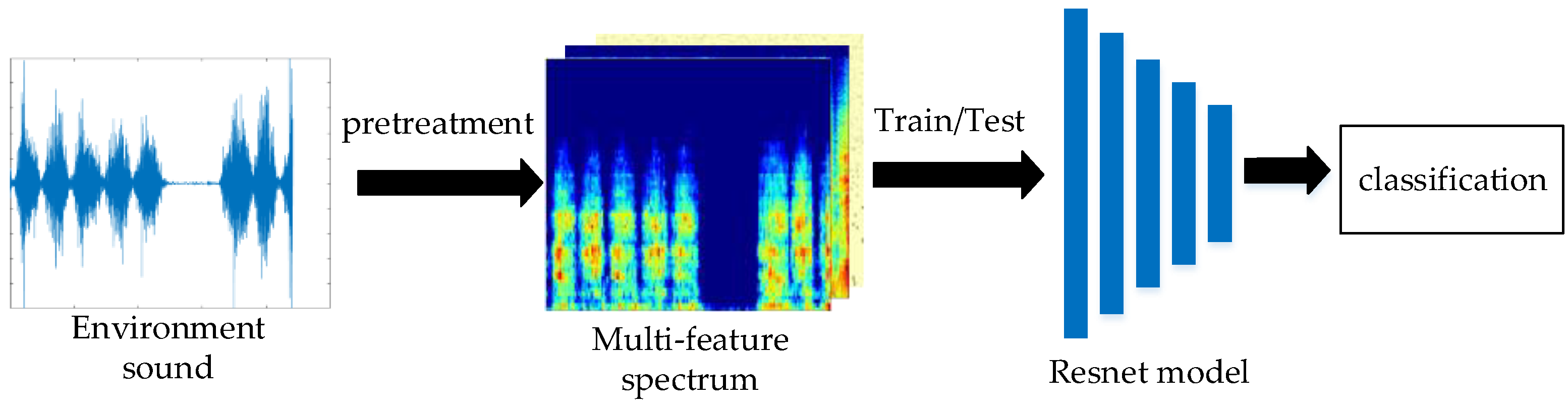
Figure 1 gives the overall design scheme of environmental sound recognition. The environmental sound is first pretreated, and in this process, the one-dimensional sound signal is mapped to two-dimensional image features, which are then entered into the residual network for training/testing, and the final result is the category information of the sound.
3.1. Feature Extraction
It is difficult to capture the useful information from original one-dimensional audio data due to a large amount of noise. In order to solve this problem, the popular method is mapping the audio data into Log-Mel spectrogram or MFCC spectrogram. Log-Mel spectrogram is designed by imitating the auditory system of the human ear. It takes the short-time Fourier transform of the sound signal and maps its frequency to the Mel frequency. However, Log-Mel spectrogram does not contain the phase information, which is an important feature of the sound signal. Therefore, it will lead to incomplete sound features and is not the optimal solution using Log-Mel spectrogram as the input of the sound recognition system. For further improving the recognition ability, the phase spectrogram of the sound is used as additional information and combines the Log-Mel spectrogram and time–frequency spectrogram as the input of neural network.
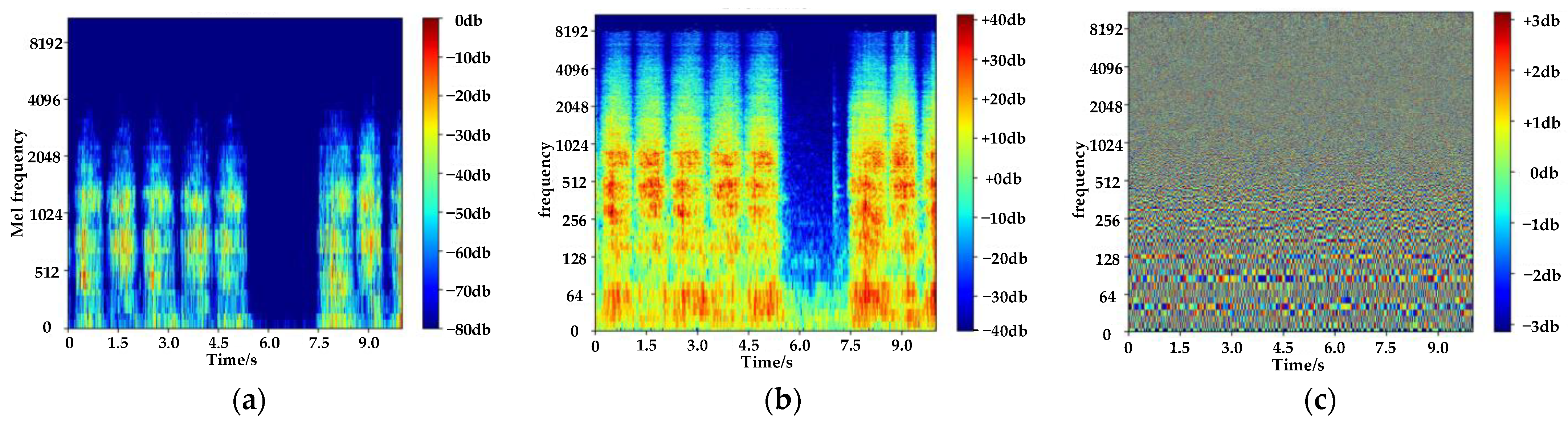
In order to obtain Log-Mel spectrogram and absolute phase spectrogram of the sound, the sound signal is subjected to short-time Fourier transform and the steps are as follows: first, the input audio signal x(n) is divided into multiple short-time parts, length of each part is 43 ms, and the part shift is 21 ms. Then, each short-time part is multiplied by the Hamming Window to improve the continuity. Finally, a 1024-point Fast Fourier Transform is performed on each part, and a feature map containing time, frequency, amplitude, and phase is obtained, where magnitude and phase are combined in complex numbers. Complex features cannot be directly fed into the neural network. Therefore, this paper separates the complex-valued spectrogram D into its magnitude (S) and phase (P) components. The matrix S and P are the time-spectrogram and the phase-spectrogram of the signal, respectively. The matrix S is subjected to a Mel-filter and logarithmic operation to obtain a Log-Mel spectrogram. Figure 2 shows three spectrograms of saw wood sound.
3.2. Residual Model
The residual network bypasses some processing layers by means of additional Skip Connections, merges their input and output, and solves the gradient exploding problem and the gradient vanishing problem of deep neural networks.
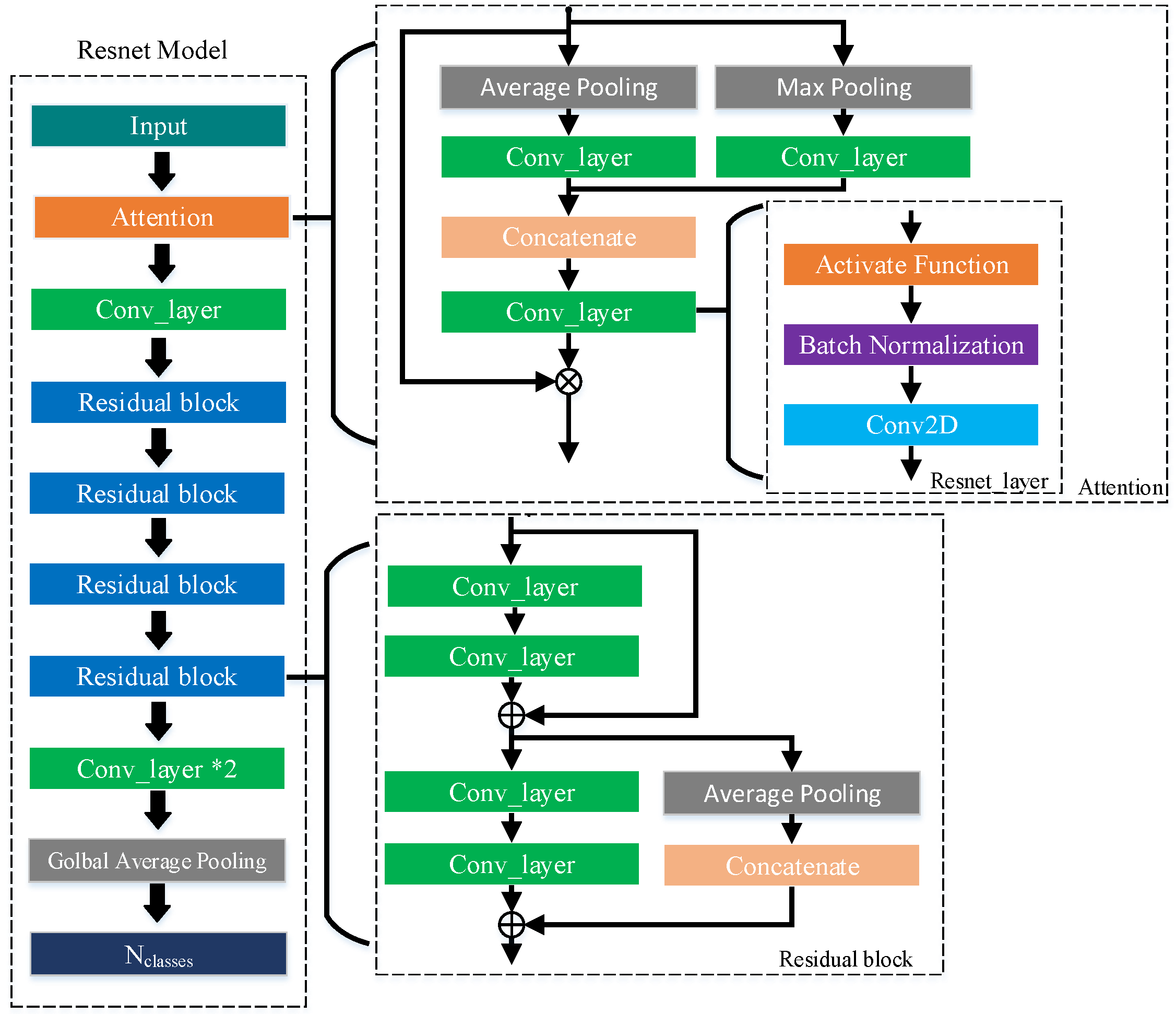
The proposed network structure (as shown in Figure 3) mainly consists of a time-frequency attention module and four residual blocks. The input data is composed of Log-Mel, Phase, and a time–frequency spectrogram connected in parallel in a new dimension. The size is , where is the frequency dimension, is the time dimension of the feature map, and is the category dimension of the feature degree. The input data passes first through the attention module, where a preliminary processing of the feature map takes place to mitigate the influence of the noise and irrelevant frequency bands in the audio. After that, it is processed by the first Conv_layer (convolution kernel 3 × 3 × 24, stride [1,2]), and then features are extracted through four residual blocks, each of which consists of two Conv_layers (convolution kernel 3 × 3 × (24 × 2n), where n is the Residual block number, stride [1,2]), two Conv_layers (convolution kernel 3 × 3 × (24 × 2n), where n is the Residual block number, stride = 1), and one Average Pooling. To ensure that the dimension of the feature map passing through the Average Pooling branch is consistent with the main route, the channel axis is zeroized after Average Pooling. Finally, the category information is obtained after going through two Conv_layers and one Global Average Pooling layer.
It is noteworthy that although the time–frequency attention structure is simple, requiring no complex computations, it does improve the recognition ability of this model. Its expression is:
, a feature vector of dimension , is input into the time–frequency attention mechanism module. First, average pooling and maximum pooling are performed on this vector in the feature channel dimension, and then it goes through two-dimensional convolution of a convolution kernel size of 1 × 1 × , and this produces two feature maps of size . The two feature maps are connected in parallel in the channel dimension, and go through two-dimensional convolution of a convolution kernel of size 1 × 1 × . This gives attention weight coefficients of size , which are multiplied by the input feature to produce the feature vector, which has been extracted by attention.
Where, is the number of neurons, and is the convolution operation, whose formula is shown (2).
where is the output of the convolution operation, is the activation functions, is the convolution kernel, is the convolution operation, is the current input feature, and is the bias.
4. Experiment and Analysis
This section describes the details of the experiment, including the datasets, the division between the training set and the validation set, and the actual parameters for the model training experiment. At the same time, several comparative experiments have been performed that demonstrate the superiority of the proposed method. The influence of feature map combination parameters, sampling rate, and time–frequency attention mechanism addition position on the experimental results is also discussed.
4.1. Datasets
This simulation experiment made use of three recognized general sound datasets: ESC10, ESC50 [21], and UrbanSound8K [22].
ESC10/ESC50: The ESC10 dataset consists of 400 environmental recordings from 10 categories, such as dog barks and rain sounds. Each sample lasts 5 s, with a sampling frequency of 44.1 KHz. The ESC50 dataset consists of keyboard sounds, clock ticks, baby crying, and more, with a total of 2000 environmental recordings from 50 categories and each sample being 5 s at a sampling frequency of 44.1 KHz. These two datasets have been divided into five parts by the authors, so 5-fold cross-validation [21] was followed in this study.
UrbanSound8K: The UrbanSound8K dataset is in wide use for automatic urban sound classification and recognition. This dataset consists of 8732 sound clips (mono and stereo), with a duration of less than 4 s, from 10 categories, including air conditioner sound, hole drilling, engine idling, gunshots, etc., at a sampling rate of 48K, 44.1 K, and 16 K. Due to the different duration and sampling rate of each sound sample, for the purpose of this study, all sound data were resampled at 44.1 KHz, and the duration of the samples were made equal to 4 s. The samples longer than 4 s were truncated, while those less than 4 s were randomly complemented.
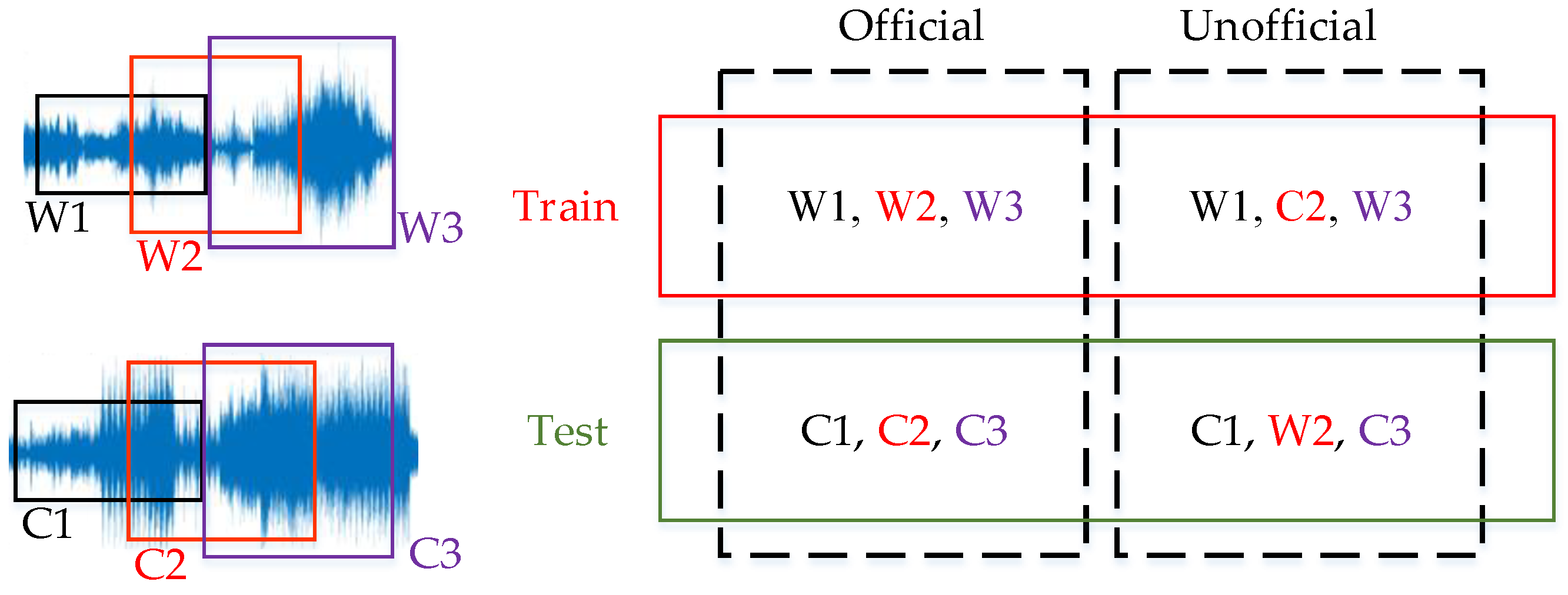
For the UrbanSound8K dataset, there are two ways of dividing the dataset: official and unofficial. The final outcome is dependent on the way of division, which makes the results of many papers incomparable to other papers [23]. The UrbanSound8K dataset takes the data in the Freesound project by sliding windows, with each window providing 50% overlap. The officially divided sample training set and test set come from different original audio files, so the training set and test set share nothing. In the case of unofficially divided sets, it is hard to make certain that the intersection of the training set and the test set is an empty set. In Figure 4, W1, W2, and W3 are training sets; C1, C2, and C3 are test sets, and this division involves no overlap. On the other hand, if W1, C2, and W3 are training sets, and C1, W2, and C3 are test sets, then W1 and W3 in the training set overlap with W2 in the test set. This apparently increases the recognition accuracy of the network, but this is not representative of the actual situation and should therefore not be applied to the training data.
4.2. Model Training
The experimental framework was TensorFlow and Keras. The entire network was constructed with TensorFlow as the bottom layer and Keras as the backend. The models and algorithms were implemented with the programming language Python3.6. Optimizing iterative model parameters was performed on a GeForce RTX 2080Ti GPU. The initial learning rate was set to be 0.001, and learning rate WarmRestart was performed with the Cosine Annealing method [24]. The learning rate was dynamically adjusted. The learning rate was initialized when 3, 7, 15, 31, 63, 127, 255, 511, or 1022 iterations were completed. The loss function was expressed in binary cross entropy. The optimization function was based on SGD. Each batch was trained on 64 data, and there were a total of 1024 rounds of training. In the training phase, the following data augmentation methods were applied: time-domain Random Cropping and Mixup [25]. The former effectively enhanced the expression ability of individual samples, while the latter enhanced the expression ability between multiple samples.
4.3. Comparative Experiment
4.3.1. Experimental Results of Feature Map Parameters
The two-dimensional convolution neural network calls for artificial extraction of manual features from the waveform, unlike the one-dimensional convolution neural network, which involves direct inputting of the waveform. The experimental parameters for extracting manual features have a great influence on environmental sound classification. In order to find the best feature map parameters, the accuracy of the network under different manual feature parameters was compared. The results with using different combinations of feature map are listed in Table 1.
The best performance happens when the Log-Mel, phase, and time–frequency spectrogram are combined as the feature map input. Individually, as the feature input, the Log-Mel spectrogram behaves significantly higher than other types of feature maps. Comparing the results of the Log-Mel spectrogram, phase spectrogram and Log-Mel, phase, and time–frequency spectrogram, it can be seen that the phase spectrogram alone is not enough to support effective environmental sound recognition. Using the phase spectrogram in conjunction with another spectrogram can improve the network’s recognition ability. Using the phase spectrogram and time–frequency spectrogram as complementary features of the Log-Mel spectrogram has the potential of achieving excellent results.
This paper evaluates the influence of audio sampling frequency on environmental sound classification. With the Log-Mel, phase, and time–frequency spectrogram combined as the network input, comparative experiments were carried out at sampling frequencies of 8 KHz, 16 KHz, 44.1 KHz, and 48 KHz. The results are shown in Table 2. At the sampling frequency of 44.1KHz, the proposed network gives the best results, scoring 97.25%, 89.00%, and 83.45% on the ESC10, ESC50, and UrbanSound8K datasets, respectively.
Using the Log-Mel spectrogram, time–frequency spectrogram, and phase spectrogram as an input and at a sampling frequency of 44.1 KHz, this paper evaluates the influence of different parameters on environmental sound classification in short-time Fourier transform. The recognition differences are shown in Table 3 for processing the sound signal using STFT with different parameters. An optimal result is yielded when the frame length is 2048 points (43 ms), the frame shift is 1024 points (21 ms), and the number of transformation points N is 2048.
4.3.2. Experimental Result Comparison of Network Models
The attention mechanism can better help the model to extract the feature information from the spectral map. Taking advantage of the improved input feature map, the model improves on previous classification performance. The effect of the insertion position of the attention mechanism is shown in Table 4.
As is suggested by the experimental results in Table 4, when the attention mechanism is put at the input end of the model, the recognition ability is the best. In this way, the feature spectrogram is first treated by the attention mechanism, and then the residual network comes in for feature extraction. The attention mechanism extracts high-dimensional features, and this effectively reduces the interference of the noise and irrelevant frequency bands in the spectrogram. When the attention mechanism is inserted into other places of the network, the low-dimensional features that have been extracted by convolution are not sensitive to attention. Additionally, the attention mechanism increases the complexity of the model. If the positive effect achieved is not enough to compensate for the penalty of the greater model complexity, the recognition ability of the model will deteriorate. Therefore, when the attention mechanism is inserted between the residual blocks, the recognition accuracy of the model decreases compared with the model without the attention mechanism. When the attention mechanism is put at the output side of the model, the effect is not significant.
Table 5 compares the proposed environmental sound recognition method and the current advanced methods, both at the optimal feature combination and network model. As can be seen in Table 5, the proposed method performs better than other methods on the ESC10, ESC50, UrbanSound8K (official/unofficial) datasets. The proposed model possesses outstanding recognition ability in environmental sound recognition.
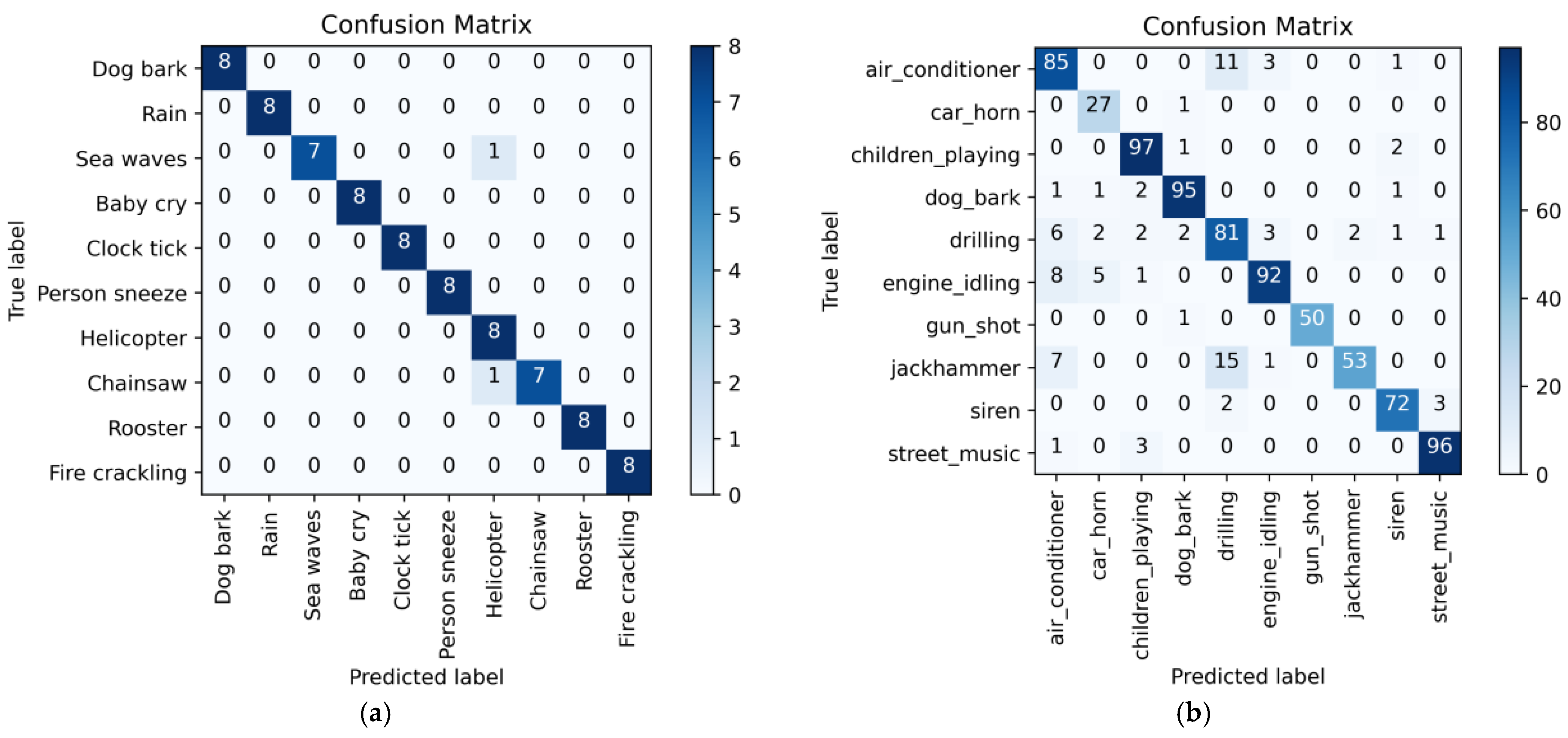
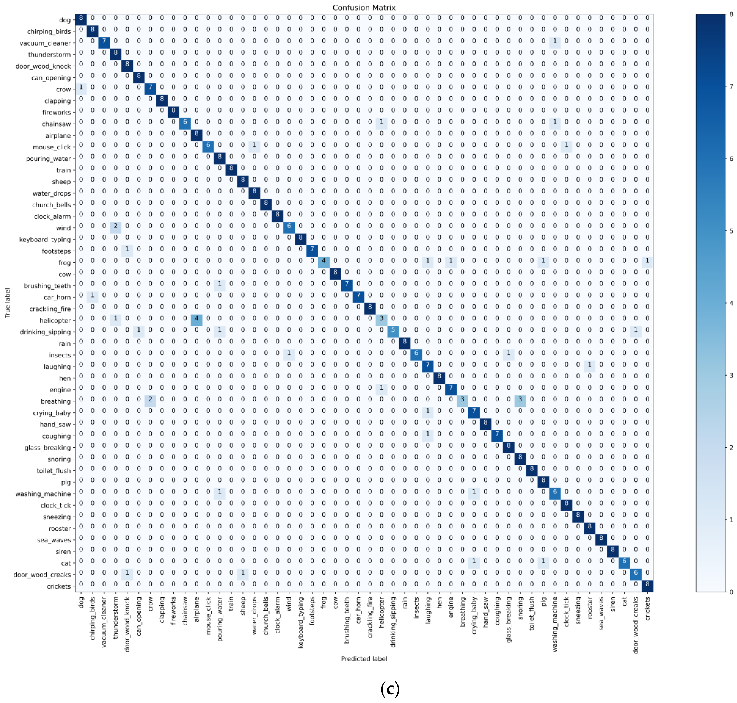
The confusion matrices of the experimental results on the ESC10 dataset, ESC50 dataset, and UrbanSound8K dataset are shown in Figure 5a–c, respectively. It can be seen that with these three datasets, the network is more sensitive to instantaneous and short-lasting sound signals, and is therefore more accurate in picking out such sound signals like gunshots and car horns. It is less sensitive to sound signals widely distributed on the time domain axis, such as engine roar, electric drill sound, and air conditioner sound. The energy of these sounds is mostly concentrated in the low-frequency end, which makes it difficult for the network to recognize them accurately.
5. Conclusions
An environmental sound classification method based on attention mechanism and multi-feature data enhancement is proposed. The phase spectrogram is added to the input feature as the phase feature supplement of the Log-Mel spectrogram, which enhances the feature expression ability and improves the robustness and generalizability of the network. Regarding the neural network, a residual network model based on attention mechanism is proposed. The attention mechanism is inserted into the beginning of the network model, so that the entire feature map is reconstructed at the input end of the network, which reduces the impact of noise on the network.
Comparative experiments were performed on the ESC10, ESC50, and UrbanSound8K datasets using the k-fold cross-validation technique. The experimental results suggest that the proposed environmental sound recognition method is effective in improving the accuracy of environmental sound recognition and possesses a prominent recognition ability in the field of environmental sound recognition.
Author Contributions
Conceptualization, J.G., C.L., Z.S., J.L. and P.W.; methodology, J.G., C.L. and Z.S.; software, J.G. and C.L.; investigation, J.G., C.L., Z.S. and P.W.; writing, J.G. and C.L. All authors have read and agreed to the published version of the manuscript.
Funding
This research was partly funded by the National Science Foundation of China (No.61901419 and No. 62101512).
Institutional Review Board Statement
Not applicable.
Informed Consent Statement
Not applicable.
Data Availability Statement
The data presented in this study are available on request from the corresponding author.
Conflicts of Interest
The authors declare no conflict of interest.
References
- Baum, E.; Harper, M.; Alicea, R.; Ordonez, C. Sound identification for fire-fighting mobile robots. In Proceedings of the IEEE International Conference on Robotic Computing, Laguna Hills, CA, USA, 31 January–2 February 2018; pp. 79–86. [Google Scholar]
- Wang, J.C.; Lee, H.P.; Wang, J.F.; Lin, C.B. Robust environmental sound recognition for home automation. IEEE Trans. Autom. Sci. Eng. 2008, 5, 25–31. [Google Scholar] [CrossRef]
- Radhakrishnan, R.; Divakaran, A.; Smaragdis, A. Audio analysis for surveillance applications. In Proceedings of the IEEE Workshop on Applications of Signal Processing to Audio and Acoustics, New Paltz, NY, USA, 16–19 October 2005; pp. 158–161. [Google Scholar]
- Cotton, C.V.; Ellis, D. Spectral vs. spectro-temporal features for acoustic event detection. In Proceedings of the 2011 IEEE Workshop on Applications of Signal Processing to Audio and Acoustics (WASPAA), New Paltz, NY, USA, 16–19 October 2011; pp. 69–72. [Google Scholar]
- Shi, Y.; Li, Y.Q.; Cai, M.L.; Zhang, X.D. A Lung Sound Category Recognition Method Based on Wavelet Decomposition and BP Neural Network. Int. J. Biol. Sci. 2019, 15, 195–207. [Google Scholar] [CrossRef] [PubMed]
- Geiger, J.T.; Helwani, K. Improving event detection for audio surveillance using Gabor filterbank features. In Proceedings of the 2015 23rd European Signal Processing Conference (EUSIPCO), Nice, France, 31 August–4 September 2015; pp. 714–718. [Google Scholar]
- Wang, J.C.; Wang, J.F.; He, K.W.; Hsu, C.S. Environmental sound classification using hybrid SVM/KNN classifier and MPEG-7 audio low-level descriptor. In Proceedings of the International Joint Conference on Neural Networks, Vancouver, BC, Canada, 16–21 July 2006; pp. 1731–1735. [Google Scholar]
- Ye, J.; Kobayashi, T.; Masahiro, M. Urban sound event classification based on local and global features aggregation. Appl. Acoust. 2017, 117, 246–256. [Google Scholar] [CrossRef]
- Bisot, V.; Serizel, R.; Essid, S.; Richard, G. Feature learning with matrix factorization applied to acoustic scene classification. IEEE/ACM Trans. Audio Speech Lang. Process. 2017, 25, 1216–1229. [Google Scholar] [CrossRef]
- Zhang, Y.; Wang, Y.; Zhou, G.; Jin, J.; Cichocki, A. Multi-kernel extreme learning machine for EEG classification in brain-computer interfaces. Exp. Syst. Appl. 2017, 96, 2. [Google Scholar] [CrossRef]
- Li, C.; Li, S.; Gao, Y.; Zhang, X.; Li, W. A Two-stream Neural Network for Pose-based Hand Gesture Recognition. IEEE Trans. Cogn. Dev. Syst. 2021, 1–10. [Google Scholar] [CrossRef]
- Tokozume, Y.; Harada, T. Learning environmental sounds with end-to-end convolutional neural network. In Proceedings of the 2017 IEEE International Conference on Acoustics, Speech and Signal Processing (ICASSP), New Orleans, LA, USA, 5–9 March 2017; pp. 2721–2725. [Google Scholar]
- Dai, W.; Dai, C.; Qu, S.; Li, J.; Das, S. Very deep convolutional neural networks for raw waveforms. In Proceedings of the IEEE International Conference on Acoustics, Speech and Signal Processing (ICASSP), New Orleans, LA, USA, 5–9 March 2017; pp. 421–425. [Google Scholar]
- Zhu, B.; Xu, K.; Wang, D.; Zhang, L.; Li, B.; Peng, Y. Environmental sound classification based on multi-temporal resolution convolutional neural network combining with multi-level features. In Advances in Multimedia Information Processing—PCM 2018, Proceedings of the Pacific Rim Conference on Multimedia, Hefei, China, 21–22 September 2018; Springer: Cham, Switzerland, 2018; pp. 528–537. [Google Scholar]
- Abdoli, S.; Cardinal, P.; Koerich, A.L. End-to-end environmental sound classification using a 1D convolutional neural network. Expert Syst. Appl. 2019, 2, 252–263. [Google Scholar] [CrossRef]
- Chu, S.; Narayanan, S.; Kuo, C.-C.J. Environmental Sound Recognition with Time–Frequency Audio Features. IEEE Trans. Audio Speech Lang. Process. 2009, 17, 1142–1158. [Google Scholar] [CrossRef]
- Piczak, K.J. Environmental sound classification with convolutional neural networks. In Proceedings of the 25th International Workshop on Machine Learning for Signal Processing, Boston, MA, USA, 17–20 September 2015; pp. 1–6. [Google Scholar]
- Salamon, J.; Bello, J.P. Deep convolutional neural networks and data augmentation for environmental sound classification. IEEE Signal Process. Lett. 2017, 24, 279–283. [Google Scholar] [CrossRef]
- Zhang, Z.; Xu, S.; Cao, S.; Zhang, S. Deep convolutional neural network with mixup for environmental sound classification. In Pattern Recognition and Computer Vision. PRCV 2018, Proceedings of the Chinese Conference PRCV, Guangzhou, China, 23–26 November 2018; Springer: Cham, Switzerland, 2018; pp. 356–367. [Google Scholar]
- Dong, X.; Yin, B.; Cong, Y.; Du, Z.; Huang, X. Environment sound event classification with a two-stream convolutional neural network. IEEE Access 2020, 8, 125714–125721. [Google Scholar] [CrossRef]
- Piczak, K.J. ESC: Dataset for environmental sound classification. In Proceedings of the 23rd ACM International Conference on Multimedia, Brisbane, Australia, 26–30 October 2015; pp. 1015–1018. [Google Scholar]
- Salamon, J.; Jacoby, C.; Bello, J.P. A dataset and taxonomy for urban sound research. In Proceedings of the 22nd ACM International Conference on Multimedia, Orlando, FL, USA, 3–7 November 2014; pp. 1041–1044. [Google Scholar]
- Guzhov, A.; Raue, F.; Hees, J.; Dengel, A. ESResNet: Environmental Sound Classification Based on Visual Domain Models. arXiv 2020, arXiv:2004.07301. [Google Scholar]
- Loshchilov, I.; Hutter, F. SGDR: Stochastic Gradient Descent with Restarts. arXiv 2016, arXiv:1608.03983. [Google Scholar]
- Zhang, H.; Cisse, M.; Dauphin, Y.N.; Lopez-Paz, D. Mixup: Beyond empirical risk minimization. In Proceedings of the International Conference on Learning Representations, Vancouver, BC, Canada, 30 April–3 May 2018. [Google Scholar]
- Boddapati, V.; Petef, A.; Rasmusson, J.; Lundberg, L. Classifying environmental sounds using image recognition networks. Procedia Comput. Sci. 2017, 112, 2048–2056. [Google Scholar] [CrossRef]
- Wang, H.; Zou, Y.; Chong, D.; Wang, W. Learning discriminative and robust time-frequency representations for environmental sound classification. arXiv 2019, arXiv:1912.06808. [Google Scholar]
Figure 1.
Overall design scheme of environmental sound recognition.

Figure 2.
Three characteristic spectra of saw wood sound. (a) Log-Mel spectrogram. (b) time spectrogram. (c) phase spectrogram.
Figure 2.
Three characteristic spectra of saw wood sound. (a) Log-Mel spectrogram. (b) time spectrogram. (c) phase spectrogram.

Figure 3.
Schematic diagram of the network model structure.

Figure 4.
UrbanSound8K Official vs Unofficial.

Figure 5.
Confusion matrix for three datasets. (a) ESC-10. (b) UrbanSound8K. (c) ESC-50.


Table 1.
Comparison of different feature map types (accuracy, %).
| Feature Map Types | ESC-10 | ESC-50 | UrbanSound8K |
|---|---|---|---|
| Log-Mel spectrogram | 92.75 | 83.25 | 80.47 |
| Phase spectrogram | 68.25 | 62.50 | 53.18 |
| time–frequency spectrogram | 90.25 | 80.75 | 78.15 |
| Phase, time–frequency spectrogram | 81.75 | 72.00 | 68.26 |
| Log-Mel, time–frequency spectrogram | 93.75 | 85.25 | 81.32 |
| Log-Mel, phase spectrogram | 95.00 | 86.75 | 81.63 |
| Log-Mel, Phase, time–frequency spectrogram | 97.25 | 89.00 | 83.45 |
Table 2.
Comparison of recognition ability under different sampling frequencies (accuracy, %).
| Sampling Frequency /Hz | ESC-10 | ESC-50 | UrbanSound8K |
|---|---|---|---|
| 8 K | 95.25 | 86.50 | 81.31 |
| 16 K | 95.25 | 87.25 | 80.76 |
| 44.1 K | 97.25 | 89.00 | 83.45 |
| 48 K | 96.00 | 88.50 | 79.94 |
Table 3.
Network recognition results of feature maps of different sizes.
| Frame Length | Frame Shift | Number of Mel Filters | Feature Map Size | Network Accuracy % (ESC-50) |
|---|---|---|---|---|
| 1024 | 512 | 40 | (40, 431, 3) | 86.25 |
| 1024 | 512 | 64 | (64, 431, 3) | 86.25 |
| 2048 | 512 | 64 | (64, 431, 3) | 86.75 |
| 2048 | 1024 | 64 | (64, 216, 3) | 88.25 |
| 4096 | 2048 | 64 | (64, 108, 3) | 84.00 |
Table 4.
Influence of time–frequency attention mechanism position on model recognition ability.
| Time–Frequency Attention Mechanism Insertion Position | ESC-10 | ESC-50 | UrbanSound8K |
|---|---|---|---|
| None | 95.25 | 84.25 | 80.35 |
| model input | 97.25 | 89.00 | 83.45 |
| Between Residual blocks | 95.75 | 86.25 | 80.35 |
| model output | 95.25 | 85.75 | 81.26 |
| model input, output and Between Residual blocks | 92.50 | 82.25 | 78.66 |
Table 5.
Comparison of algorithms in the ESC10, ESC50, and UrbanSound8K datasets.
| Model | ESC10 | ESC50 | UrbanSound8K (Official) | UrbanSound8K (Unofficial) |
|---|---|---|---|---|
| EnvNet [11] | 88.10 | 74.10 | 71.10 | - |
| EnvNet v2 [12] | 91.30 | 84.70 | 78.30 | - |
| GoogLeNet [26] | 86.00 | 73.00 | - | 93.00 |
| VGG-like CNN + mixup [19] | 91.70 | 83.90 | 83.70 | - |
| TFNet (no aug.) [27] | 93.10 | 86.20 | - | 88.50 |
| ESResNet-Attention [23] | 94.25 | 83.15 | 82.76 | 98.18 |
| Ours | 97.25 | 89.00 | 83.45 | 98.25 |
Publisher’s Note: MDPI stays neutral with regard to jurisdictional claims in published maps and institutional affiliations. |
© 2022 by the authors. Licensee MDPI, Basel, Switzerland. This article is an open access article distributed under the terms and conditions of the Creative Commons Attribution (CC BY) license (https://creativecommons.org/licenses/by/4.0/).
Share and Cite
MDPI and ACS Style
Guo, J.; Li, C.; Sun, Z.; Li, J.; Wang, P. A Deep Attention Model for Environmental Sound Classification from Multi-Feature Data. Appl. Sci. 2022, 12, 5988. https://0-doi-org.brum.beds.ac.uk/10.3390/app12125988
AMA Style
Guo J, Li C, Sun Z, Li J, Wang P. A Deep Attention Model for Environmental Sound Classification from Multi-Feature Data. Applied Sciences. 2022; 12(12):5988. https://0-doi-org.brum.beds.ac.uk/10.3390/app12125988
Chicago/Turabian StyleGuo, Jinming, Chuankun Li, Zepeng Sun, Jian Li, and Pan Wang. 2022. "A Deep Attention Model for Environmental Sound Classification from Multi-Feature Data" Applied Sciences 12, no. 12: 5988. https://0-doi-org.brum.beds.ac.uk/10.3390/app12125988
Note that from the first issue of 2016, this journal uses article numbers instead of page numbers. See further details here.