Modification of Segment Structure Calculation Theory and Development and Application of Integrated Software for a Shield Tunnel

Featured Application

The calculation software developed in this paper, as the shield tunnel segment structure design calculation software, can provide calculation tools for shield tunnel structure design engineers to improve design efficiency and reduce design costs.

Abstract

From the aspect of calculation theory, the beam–spring model method and modified routine method of shield tunnel segment structure calculation were improved, and an efficient integrated software system for segment structure calculation of shield tunnel was developed. The beam–spring method is generally calculated according to the assumption of continuous displacement between beams and joints, and the existing modified routine method assumes that the lateral pressure gradient is constant generally, which does not consider the variation in lateral pressure gradient caused by the difference in the lateral pressure coefficient of soil layers or the water level height, which has a certain deviation from the actual situation. The existing beam–spring method and modified routine method theory were improved, the discontinuous displacement between beams and joints in the beam–spring method was taken into account, and the problem of lateral pressure gradient change in the modified routine method was solved. The calculation software system developed by C# and python programming language was proposed to improve the accuracy and efficiency of segment structure calculation. Based on the actual monitoring data of the internal force of the shield tunnel segment and the adjacent shield tunnel segments under construction in Changsha, China, the segments of the shield tunnel with different cross-section sizes and different hydrogeological conditions are calculated to verify the reliability of the calculation software system. At the same time, combined with the calculation results of the software system and field test data, the stiffness reduction coefficient and equivalent foundation resistance coefficient in the modified routine method were derived to further improve the accuracy of the calculation results, which provided a new idea for the calculation of segment structure of shield tunnel with different diameters under different hydrogeological conditions.

1. Introduction

The lining structure of the shield tunnel is composed of concrete segments and joint bolts. Based on a different structural assumption of lining segments [1], the internal force calculation method of the shield lining structure is mainly divided into the free form deformation method, the elastic support method, the ground-structure method, the modified routine method, and the beam–spring model method. Huang Qingfei et al. [2] deduced the theoretical solution of the internal force of each segment under the condition of lateral pressure with gradient variation from the existing modified routine method and studied the influence of the water level change on the internal force of the segments under different geological conditions. Zhang Meicong et al. [3] used a modified routine method to analyze the internal forces of circular shield tunnel lining segments. Wang Zhiliang and Peng Yicheng et al. [4] calculated the bending moment of the segments with joint bolts under fully elastic conditions in combination with a modified routine method to study the influence of the transverse deformation of the tunnel on the safety of the tunnel structure and proposed effective value of bending stiffness from the perspective of numerical simulation and theoretical derivation. Regarding the problem that the current beam–spring model cannot simulate the deformation discontinuity of the shield segment joints precisely, many scholars worldwide [5,6,7,8,9] researched the applicability of the beam–spring method in a segment structure design. The mechanical properties adopted during the calculation of the segment joint have significant impacts on the force and deformation of segment structures, and the calculation accuracy of the beam–spring method depends on the selection of input parameters. Scholars proposed the method for parameter determination of the rotational stiffness of segment joints with corresponding mechanical models based on theoretical analysis, numerical simulation, joint tests, etc. In the aspect of field model test for studying mechanical properties of segments, the test model [10] of the segment lining structure is designed by using a shield tunnel-ground simulation facility and a rotary water pressure device to control the water pressure and the earth pressure separately, based on the ground-structure model; the photoelastic model test is given in reference [11], which promoted the development of shield tunnel segment structure design.

Zhu Hehua et al. [12] summarized the mechanical models describing the rotational stiffness value of the joints based on test results, including linear, bilinear, and nonlinear models, as well as the beam–spring continuous model, which uses a continuous spring to simulate the segment joint, assuming joint displacements of adjacent segments at the joint position are consistent. However, there is a significant mismatch between the calculation and measurements of force and deformation of the shield segment lining on the beam–spring continuous model. The beam–joint model [13] ought to have the same stiffness matrix of the joint node force and displacement as the beam–spring discontinuous model, which is more in line with the actual situation in the calculation results.

Therefore, on the basis of previous studies, this article improved the existing beam–spring method and modified the routine method theory, taking into account the discontinuity of the beam–joint deformation in the beam–spring model and the lateral pressure gradient change in the modified routine method. The calculation software system developed by C# and the python programming language are proposed to improve the accuracy and efficiency of segment structure calculation.

2. Calculation Theory Revision

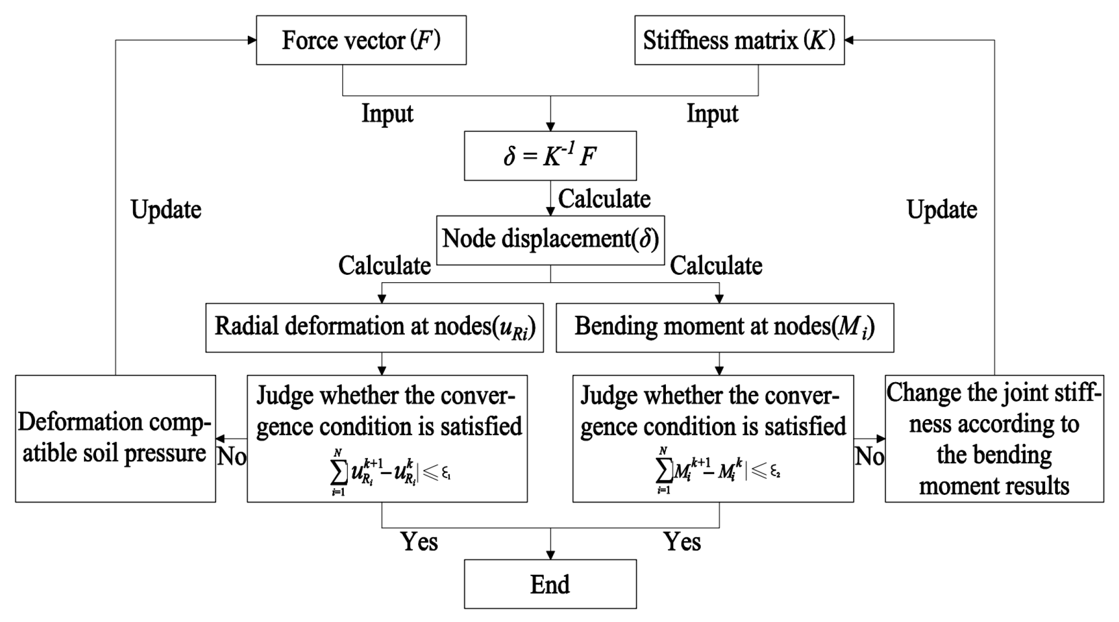
2.1. Beam–Spring Method

The beam–spring method simplifies the main section of the segment to a circular arc beam or a linear beam frame, regarding the segment joint as a rotating spring and the ring joint as a structural model of a shear spring, and using the finite element method for elastic analysis. Murakami and Koizumi added the effect of staggered joints to the elastic hinge ring model and used springs to evaluate the shear resistance between the rings to explain the rotation and shearing resistance of the segment joint. They proposed an analytical method (also known as the M-K method) for the shear effect of tube segment longitudinal joints [1]. This model also considers the stiffness of the segment joints, the joint position, and the effect of the staggered joint assembly, which is a reasonable calculation model, as shown in Figure 1.

This calculation model includes a multi-hinged ring calculation method and a uniform stiffness ring algorithm. At the same time, the shear stiffness of the segment ring joint can be used to characterize the splicing effect of the staggered joint, which is an effective method of explaining the load-bearing mechanism of the pipe ring [14,15,16,17,18,19]. During the calculation, despite that the existing related beam–spring model stiffness matrix, coordinate transformation, formation reaction research, and calculation program development all assumed that the beam–joint displacement is continuous, but this paper considers the beam–joint deformation in the beam–spring model to be discontinuous, the derivation process is as follows:

Divide the tube of shield tunnel into N straight beam section with equal length l and central angle of θ, then:

$$\theta =\frac{2\pi }{N},l=2rsin(\frac{\theta }{2})$$

(1)

where r is the radius of the tunnel section.

By considering the angle changes in different beam elements, the vertical and lateral distributed forces acting on each beam element are converted into equivalent node forces.

2.1.1. Apply the Vertical Distributed Forces

If only the vertical distributed force p(x) is applied, the structural analysis diagram is shown in Figure 2. θ₁ is the angle between the unit and the horizontal direction, and the angle between the vertical distributed force and the unit is $\frac{\pi }{2}-{\theta }_1$. (x₁,y₁) and (x₂,y₂) are the coordinates of node 1 and node 2, and then:

$$x_2=x_1+lcos({\theta }_1),y_2=y_1+lsin({\theta }_1)$$

(2)

The vertical force p(x) is equivalent to horizontal and vertical component forces to calculate the equivalent internal structural forces. The derivation is shown as:

$$\begin{array}{l}{N}_1^p={\displaystyle {\int }_{x_1}^{x_2}p(x)\cos (\pi /2-{\theta }_1)A_1(\frac{x-x_1}{\cos ({\theta }_1)})}dx\\ Q_1^p={\displaystyle {\int }_{x_1}^{x_2}p(x)\sin (\pi /2-{\theta }_1)H_1(\frac{x-x_1}{\cos ({\theta }_1)})}dx\\ M_1^p={\displaystyle {\int }_{x_1}^{x_2}p(x)\sin (\pi /2-{\theta }_1)H_2(\frac{x-x_1}{\cos ({\theta }_1)})}dx\\ N_2^p={\displaystyle {\int }_{x_1}^{x_2}p(x)\cos (\pi /2-{\theta }_1)A_2(\frac{x-x_1}{\cos ({\theta }_1)})}dx\\ Q_2^p={\displaystyle {\int }_{x_1}^{x_2}p(x)\sin (\pi /2-{\theta }_1)H_3(\frac{x-x_1}{\cos ({\theta }_1)})}dx\\ M_2^p={\displaystyle {\int }_{x_1}^{x_2}p(x)\sin (\pi /2-{\theta }_1)H_4(\frac{x-x_1}{\cos ({\theta }_1)})}dx\end{array}$$

(3)

where

A₁(x) is the interpolation function of the axial displacement at node 1, $A_1(x)=1-\frac{x}{l}$;

A₂(x) the interpolation function of the axial displacement at node 2, $A_2(x)=\frac{x}{l}$;

H₁(x) is the horizontal displacement interpolation function of node 1 (Vertical to the beam), $H_1(x)=1-\frac{3}{l^2}{x}^2+\frac{2}{l^3}{x}^3$;

H₂(x) is the interpolation function of the corner at node 1, $H_2(x)=x-\frac{2}{l}{x}^2+\frac{1}{l^2}{x}^3$;

H₃(x) is the horizontal displacement interpolation function of node 2 (Vertical to the beam), $H_3(x)=\frac{2}{l^2}{x}^2-\frac{1}{l^3}{x}^3$;

H₄(x) is the interpolation function of the corner at node 2, $H_4(x)=-\frac{1}{l}{x}^2+\frac{1}{l^2}{x}^3$.

2.1.2. Apply the Horizontal Distributed Forces

If only the horizontal distributed force q(y) is applied, the structural analysis diagram is shown in Figure 3, and the included angle between the element and horizontal force is $\pi -{\theta }_1$.

The laterally distributed force q(y) is equivalent to horizontal and vertical component forces to calculate the equivalent node forces. The derivation is shown as:

$$\begin{array}{l}{N}_1^q={\displaystyle {\int }_{y_1}^{y_2}q(y)\cos (\pi -{\theta }_1)A_1(\frac{y-y_1}{\sin ({\theta }_1)})}dy\\ Q_1^q={\displaystyle {\int }_{y_1}^{y_2}q(y)\sin (\pi -{\theta }_1)H_1(\frac{y-y_1}{\sin ({\theta }_1)})}dy\\ M_1^q={\displaystyle {\int }_{y_1}^{y_2}q(y)\sin (\pi -{\theta }_1)H_2(\frac{y-y_1}{\sin ({\theta }_1)})}dy\\ N_2^q={\displaystyle {\int }_{y_1}^{y_2}q(y)\cos (\pi -{\theta }_1)A_2(\frac{y-y_1}{\sin ({\theta }_1)})}dy\\ Q_2^q={\displaystyle {\int }_{y_1}^{y_2}q(y)\sin (\pi -{\theta }_1)H_3(\frac{y-y_1}{\sin ({\theta }_1)})}dy\\ M_2^q={\displaystyle {\int }_{y_1}^{y_2}q(y)\sin (\pi -{\theta }_1)H_4(\frac{y-y_1}{\sin ({\theta }_1)})}dy\end{array}$$

(4)

The equivalent node force of node 1 and node 2 in the local coordinate system is:

$$\left\{\begin{array}{c}{F}_1^{\mathrm{L}}\\ F_2^{\mathrm{L}}\end{array}\right\}=\left\{\begin{array}{l}{N}_1\hfill \\ Q_1\hfill \\ M_1\hfill \\ N_2\hfill \\ Q_2\hfill \\ M_2\hfill \end{array}\right\}=\left\{\begin{array}{l}{N}_1^p\hfill \\ Q_1^p\hfill \\ M_1^p\hfill \\ N_2^p\hfill \\ Q_2^p\hfill \\ M_2^p\hfill \end{array}\right\}+\left\{\begin{array}{l}{N}_1^q\hfill \\ Q_1^q\hfill \\ M_1^q\hfill \\ N_2^q\hfill \\ Q_2^q\hfill \\ M_2^q\hfill \end{array}\right\}$$

(5)

where $F_1^{\mathrm{L}}$ is the equivalent node force of node 1 in the local coordinate system, $F_1^{\mathrm{L}}=[N_1 Q_1 M_1{]}^T$;$F_2^{\mathrm{L}}$ is the equivalent node force of node 2 in the local coordinate system, and $F_2^{\mathrm{L}}=[N_2 Q_2 M_2{]}^T$.

The stiffness matrix of the beam in global coordinate is:

$${\left[K^{1,G}\right]}_{6\times 6}=\left[\begin{array}{cc}{k}_{11}^{1,G}& k_{12}^{1,G}\\ k_{21}^{1,G}& k_{22}^{1,G}\end{array}\right]=\left[T\right]\left[\begin{array}{cc}{k}_{11}& k_{12}\\ k_{21}& k_{22}\end{array}\right]{\left[T\right]}^T$$

(6)

where [k₁₁], [k₁₂], [k₂₁], and [k₂₂] are nodal stiffness matrices, according to beam–spring model researches [20]. [T] is the coordinate transformation matrix:

$$\left[T\right]=\left[\begin{array}{cc}{T}_1& \\ & T_2\end{array}\right],\left[T_i\right]=\left[\begin{array}{ccc}\cos {\alpha }_i& -\sin {\alpha }_i& 0\\ \sin {\alpha }_i& \cos {\alpha }_i& 0\\ 0& 0& 1\end{array}\right](i=1,2)$$

(7)

where ${\alpha }_i(i=1,2)$ is the angle between the arc tangent direction of nodes 1 and 2 and the X-axis. For the straight beam model, ${\alpha }_1={\alpha }_2$.

2.1.3. Overall Stiffness Matrix Assembly

When the beam–spring continuous model is adopted by using force vector integration and coordinate conversion, the vertical and lateral distributed forces acting on a beam element are transformed into equivalent nodal forces at the two ends of the element in the overall coordinate system. Then, the assembled overall stiffness matrix is:

$${\left[K_G\right]}_{3N\times 3N}=\left[\begin{array}{ccccc}{k}_{11}^{1,G}+k_{11}^{N,G}& k_{12}^{1,G}& 0& \cdots & k_{1N}^{N,G}\\ k_{21}^{1,G}& k_{22}^{1,G}+k_{22}^{2,\mathrm{G}}& k_{23}^{2,\mathrm{G}}& \cdots & 0\\ 0& k_{32}^{2,\mathrm{G}}& k_{33}^{2,\mathrm{G}}+k_{33}^{3,\mathrm{G}}& \cdots & 0\\ ⋮& ⋮& ⋮& \ddots & k_{(N-1)N}^{N-1,G}\\ k_{N1}^{N,G}& 0& 0& k_{N(N-1)}^{N-1,G}& k_{NN}^{N-1,G}+k_{NN}^{N,G}\end{array}\right]$$

(8)

${\left[K_G\right]}_{3N\times 3N}$ is an overall stiffness matrix formed by the assembly of N straight beam elements under the overall coordinate system.

The overall force vector is assembled to form the overall node force vector, as shown below.

$$F_G={\left\{\begin{array}{c}{F}_1^{N,G}+F_1^{1,G}\\ F_2^{1,G}+F_2^{2,G}\\ ⋮\\ F_N^{N-1,G}+F_N^{N,G}\end{array}\right\}}_{3N\times 1}$$

(9)

F_G is the overall nodal force vector formed by the assembly of N beam elements on the shield tunnel wall under the overall coordinate system.

During the calculation of the beam–spring discontinuity model to determine the joint displacement, joint deformation between adjacent beams is considered accordingly; the deformation discontinuity between the beam and the joint is also considered, and the joint force of the joint is calculated. Calculation examples of element 1 and element 2 are shown in Figure 4.

Node 2 of element 1 and node 2a of element 2 are in a state of static equilibrium; their displacement is different. The spring connection node 2 and 2a has axial, tangential, and rotational stiffness $k_n,k_s,k_{\theta }$. Through the nodal force expressions (3~4), combined with the second theorem of Karnowski, assuming that node 2a is fixed, the nodal force at node 2 is $F_2^{\mathrm{c}}=[N_c Q_c M_c{]}^T$, then the displacement of node 2 under the applied load can be expressed as ${[U_2 V_2 {\theta }_2]}^T$. By the state of static equilibrium, the nodal force at node 2a is calculated by the displacement matrix ${[U_2 V_2 {\theta }_2]}^T$ of node 2 and the joint stiffness, which is $F_{2a}^{\mathrm{c}}=[N_{c1} Q_{c1} M_{c1}{]}^T$. Similarly, assuming that node 2 is fixed, the nodal force at node 2a is $F_{2a}^{\mathrm{c}}=[N_{c1} Q_{c1} M_{c1}{]}^T$, then the displacement of node 2a under the applied load can be calculated, which is ${[U_{2a} V_{2a} {\theta }_{2a}]}^T$. Finally, by the state of static equilibrium, the nodal force $F_2^{\mathrm{c}}=[N_c Q_c M_c{]}^T$ of node 2 is calculated by the displacement ${[U_{2a} V_{2a} {\theta }_{2a}]}^T$ of node 2a and the joint stiffness. Then the relationship between joint force and displacement of joint element here is as follows:

$$\left\{\begin{array}{l}{N}_c\hfill \\ Q_c\hfill \\ M_c\hfill \\ N_{c1}\hfill \\ Q_{c1}\hfill \\ M_{c1}\hfill \end{array}\right\}=\left\{\begin{array}{cccccc}{k}_n& & & -k_n& & \\ & k_s& & & -k_s& \\ & & k_{\theta }& & & -k_{\theta }\\ -k_n& & & k_n& & \\ & -k_s& & & k_s& \\ & & -k_{\theta }& & & k_{\theta }\end{array}\right\}\left\{\begin{array}{l}{U}_2\hfill \\ V_2\hfill \\ {\theta }_2\hfill \\ U_{2\mathrm{a}}\hfill \\ V_{2a}\hfill \\ {\theta }_{2a}\hfill \end{array}\right\}$$

(10)

After determination of the joint force from the nodal displacement, substitute the nodal displacement and the joint force into the corresponding joint conditions (continuous, sliding, or free) between the segments. If the joint conditions are not met, modify the joint state equation for the next iteration.

It is further deduced that the stiffness matrix of the joint element is assembled as:

$${\left[K^{j,G}\right]}_{6\times 6}=\left[\begin{array}{cc}{k}_{22}^{j,G}& k_{22a}^{j,G}\\ k_{2a2}^{j,G}& k_{2a2a}^{j,G}\end{array}\right]=\left[T\right]\left[\begin{array}{cc}{k}_{22}& k_{22a}\\ k_{2a2}& k_{2a2a}\end{array}\right]{\left[T\right]}^T$$

(11)

in which $\left\{\begin{array}{c}{N}_c\\ Q_c\\ M_c\end{array}\right\}=\left[k_{22}\right]\left\{\begin{array}{c}{U}_2\\ V_2\\ {\theta }_2\end{array}\right\}$, $\left[k_{22}\right]=\left\{\begin{array}{ccc}{k}_n& & \\ & k_s& \\ & & k_{\theta }\end{array}\right\}$, $\left[k_{22}^{j,G}\right]=\left[T\right]\left[k_{22}\right]{\left[T\right]}^T$,$\left[k_{2a2a}^{j,G}\right]$ is as the same.

The N representing the number of beam elements and joint elements are assembled to form the overall stiffness matrix shown below:

$${\left[K_G\right]}_{3N\times 3N}=\left[\begin{array}{ccccc}{k}_{11}^{1,G}+k_{11}^{N,G}& k_{12}^{1,G}& 0& \cdots & k_{1N}^{N,G}\\ k_{21}^{1,G}& k_{22}^{1,G}+k_{22}^{j,G}& k_{22\mathrm{a}}^{j,G}& \cdots & 0\\ 0& k_{2\mathrm{a}2}^{j,G}& k_{2a2a}^{j,G}+k_{2a2a}^{2,\mathrm{G}}& \cdots & 0\\ ⋮& ⋮& ⋮& \ddots & k_{(N-1)N}^{N-1,G}\\ k_{N1}^{N,G}& 0& 0& k_{N(N-1)}^{N-1,G}& k_{NN}^{N-1,G}+k_{NN}^{N,G}\end{array}\right]$$

(12)

${\left[K_G\right]}_{3N\times 3N}$ is the overall stiffness matrix formed by the assembly of N beam elements and joint elements in the global coordinate system.

After the overall stiffness matrix and loading matrix of the structure are determined, the displacement of the structure can be solved accordingly. Then it is necessary to judge whether the joint force obtained by the displacement vector meets the joint conditions between segments, and finally, the radial displacement and bending moment at each node can be calculated by the iteration method.

According to the direction of the radial displacement, the state of the foundation spring could be determined to further apply the finite element iteration method. Moreover, to effectively simulate the effect of the ring joints under the staggered joint assembly in iterative calculations, the relative deformation of the lining segment forming the staggered joint angle is calculated based on the stiffness of the spring element of the ring joint. Meanwhile, calculate the circumferential and radial shear forces of adjacent ring segment joints by matrix method to check the difference between the force on the single ring segment to ensure convergence.

2.2. Modified Routine Method

The modified routine method is a typical method of the homogeneous ring method. According to the homogeneous ring method, the internal force of the tube segment is calculated elastically. Meanwhile, the stiffness reduction and bending moment distribution caused by the tube joint are considered in the calculation of the internal force of the tube segment [21].

Figure 5 shows that the existing modified routine method lateral horizontal load is in standard trapezoidal form, assuming that the lateral load gradient remains unchanged, and then the theoretical internal elastic force solution can be decomposed to the lateral load into rectangular loads and triangular-form loads for the solution.

If the formation boundary or the water level is below the top surface of the pipe ring, due to the change in the lateral pressure coefficient or the effective stress of the geosphere above and below the water level, the gradient of lateral trapezoidal load changes abruptly at the stratum boundary or water level boundary. Then the stress is not a standard trapezoidal form. It should be decomposed into three parts: rectangular load, full-span (span height equal to tunnel diameter) triangular load, and partial-span triangular load. The load diagram is shown in Figure 6.

The author of this paper derived the elastic solution of the internal force under this working condition in a previous study [2], improved the existing modified routine method accordingly, and quantitatively analyzed the influence of internal force before and after the modification.

In this paper, the calculation software system module was developed for further improvement of the modified routine method. Meanwhile, the modified idiomatic module was modified based on the measurements of each segment and the calculations of the beam–spring model. The displacement value was used as the basis for the inversion. Different bending stiffness reduction coefficients η were determined through a large number of calculations and the measured value of the internal force and the calculation of the beam–spring method module. It was determined that under a certain working condition, the bending moment adjustment coefficient ζ is constant, and the recommended value of the bending stiffness reduction coefficient η based on the calculation results in different tunnel segment positions; as the verification standard improves the accuracy and expands the scope of application of the calculation.

3. Integrated Software System Development

By considering the effect of the joint between the rings in the beam–spring model, the discontinuous deformation between the beam and the joint, and the calculation of the lateral pressure gradient change in the modified routine method, the calculation software system was developed by the C# and Python programming language. The calculation results were compared with the on-site measurements, and the stiffness reduction coefficient and the equivalent foundation resistance coefficient in the modified routine method were corrected by inversion calculated, which is embedded in the calculation software to improve the accuracy. The calculation flow of the program is shown in Figure 7.

The integrated software system included two modules: the improved modified routine method and the beam–spring method (continuous and discontinuous models). The beam–spring method modules are based on continuous and discontinuous models to form comparison results. The software inputs mainly include soil layer information (physical and mechanical parameters), segment parameters (cross-section geometry and physical mechanics), tunnel depth and groundwater level, graphical information, and the DXF (map) output options, and the outputs are mainly extracted from the internal force analysis diagram, the internal force value data table, the load calculation result table, the horizontal displacement, and the calculation of soil column height, and the output picture can be edited. The system function structure is shown in Figure 8.

The interface is shown in Figure 9.

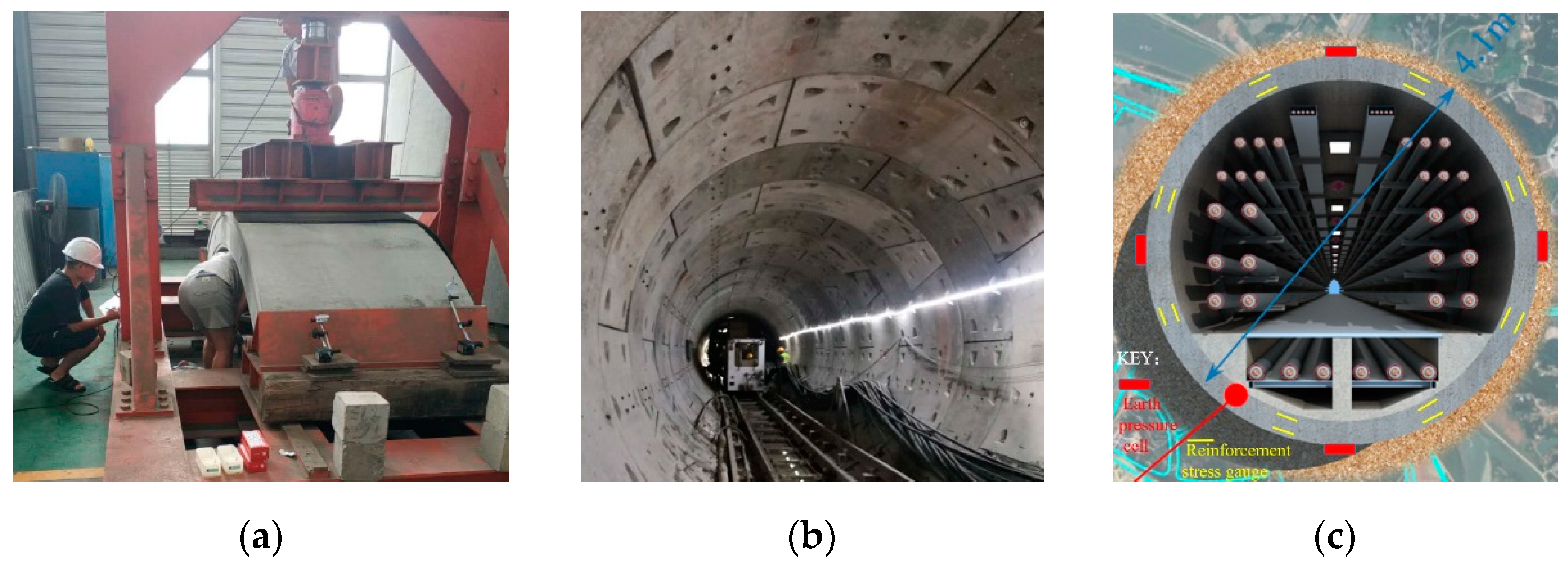
4. Calculation and Verification of a Shield Tunnel in Changsha

4.1. Model Input Parameters

The electric shield tunnel in Changsha, China, has an inner diameter of 3.6 m, an outer diameter of 4.1 m, and a segment thickness of 0.25 m. The geology of this shield tunneling mainly includes strongly weathered silty mudstone, gravel sand, fully weathered argillaceous siltstone, silty clay, and strongly weathered slate. The shield section lining adopts the following structural types:

(1)

The full ring of the lining ring is composed of a small capping block (K), two adjacent blocks (L), and three standard blocks (B). Each segment is connected by bending bolts;

(2)

Staggered stitch is used between the rings;

(3)

The minimum curve radius that can be fitted to the lining ring of R = 150 m;

(4)

Design each segment and the segmented reinforcement with different buried depths or different rock(soil)properties, respectively.

The main design parameters of the shield segment are shown in

Table 1. Main design parameters of shield segment.

Item	Parameter
Diameter	Out D φ4100 mm, Inner D φ3600 mm
Lining ring block	6 (17° × 1 + 63.5° × 2 + 72° × 3)
Lining thickness	250 mm
Lining ring width	1000 mm (150 m ≤ R < 300 m) 1200 mm (R ≥ 300 m and Straight)
Wedge	36 mm (150 m ≤ R < 300 m) 40 mm (R ≥ 300 m and Straight)
Interface	Nitrile Cork Rubber with 2 mm thickness
Material	C50, Impermeability grade P12

.

4.2. Analysis of Calculation Results

The shield tunnel segments with a buried depth of 6 m were calculated using the two modules by the software, respectively. The hydrogeological input parameters were selected according to the detailed survey parameters. The calculation results of the outer diameter of 4.1 m with a segment thickness of 0.25 m, the outer diameter of 8.2 m with a segment thickness of 0.4 m with the specific rotational stiffness, and the elastic modulus of 34.5 GPa are shown in Figure 10.

Under the same hydrogeological conditions, there is a certain difference between the calculation result of the modified routine method and the beam–spring method module. The normal pressure acting on the segment, the axial force of the segment, the bending moment, and the formation deformation was monitored to verify the rationality of the developed software module. Additionally, the data obtained from the shield tunneling test section and on-site measurements were used for inversion correction calculation of the pressure load, as the comparison reference for the continuous correction of the software input parameters, and the built-in calculation framework. The field segment data measurement is shown in Figure 11.

Table 2. The relationship between measured value of internal segment force and calculation value of software.

	On-Site	Modified Routine Method	Beam–Spring (Discontinuous)	Beam–Spring (Continuous)
Max bending moment (kN m)	34.7	32.7	39.9	45.2
Axial Force (kN)	367	319	389	412
Error of bending moment		−6.12%	+15.0%	+30.3%
Error of Axial Force		−15.0%	+6.05%	+12.3%

shows the calculation results of the shield tunnel with an outer diameter of 4.1 m and segment thickness of 0.25 m. Compared with the measured data, it is certain that the beam–spring discontinuity model and the modified routine method model after inversion and correction of the parameters improved the accuracy of the results accordingly.

By combining the above calculations and relying on the development software to calculate the segment structure of shield tunnels with different outer diameters, the calculation program uses the bending moment and displacement values of different tunnel segments on the same section as the basis for the inversion, and different tunnel segments are calculated. The bending stiffness reduction coefficient η of the lining ring can improve the similarity between the change rule of the bending moment of the lining ring at different positions and the change rule of the measured value at different positions. Based on the principle of reducing the relative error with the actual measured value and compared with the calculation result of the beam–spring method, it was concluded that the recommended bending stiffness reduction coefficient η for different parts of the shield lining ring under the hydrogeological conditions of this project is as follows shown in Figure 12.

Figure 12 shows that for a shield tunnel with variable outer diameters, the stiffness reduction coefficients within the range of 45° on both sides of the vault at the same position should select the larger value. With the increase in the outer diameter of the shield tunnel, the recommended value of the stiffness reduction coefficient of the modified routine method would gradually decrease. When the outer diameter of the shield tunnel is larger than 10.5 m, the sensitivity of the stiffness reduction coefficient changes in different lining positions decreases. The stiffness reduction coefficient of the ring can be the average of the recommended values for different lining positions.

5. Conclusions

This article mainly illustrates the connection and verification of the modified routine method and beam–spring model in the calculation of shield tunnel lining structure. The development software took into account the discontinuous displacement between the beam and the joint in the beam–spring model and verified on-site measurements to inversely calculate the stiffness reduction coefficient and equivalent foundation resistance factor in the modified routine method. Consequently, the accuracy and efficiency of the calculation of the segment structure were improved by using the method discussed above. The proposed scheme works, as the adopted load-structure method provides a solution for internal force calculation of shield tunnel structure under different engineering hydrogeological conditions, but the interaction analysis of the construction process of twin tunnels can not be considered, which needs further research. The details of the conclusions are concluded as follows:

• The calculation program based on the beam–spring method evaluating the joint effect between the segments and the discontinuous displacement between the beam and the joint can reasonably evaluate the staggered assembly of the shield tunnel segments, which is more reasonable than the beam–joint strain continuous assumption model in the mechanical behavior between segments. Through the development of the calculation program by setting analytical conditions, the joint spring stiffness can be determined reasonably, and the rationality and accuracy of the calculation of the segment structure are improved;
• The reasonable value of the stiffness reduction coefficient in the modified routine method is obtained through the inversion of the field measured data and the calculation results of the beam–spring model. A large number of software calculation results were compared with the measured data, which shows that the modified routine method calculation module of the software has high accuracy in the calculation of segment bending moment;
• The calculation parameters of shield tunnels with different cross-section diameters should be further studied with variables of hydrogeological parameters and the segment diameters. The current research shows that for shield tunnels with different segment diameters adopting recommended bending stiffness reduction coefficient for different parts of the lining ring could provide significant reference value in numerical calculation.

References

1. Murakami, H.; Koizumi, A. Study on load bearing eapacity and mechanics of shield segment ring. Proc. Jpn. Soc. Civ. Eng. 1978, 272, 103–115. [Google Scholar] [CrossRef] [Green Version]
2. Huang, Q.F.; Yuan, D.J.; Wang, M.S. Influence of water level on internal force of segments of shieldtunnels. Chin. J. Geotech. Eng. 2008, 30, 1112–1120. [Google Scholar]
3. Zhang, M.C. Analysis of lining segments for circular shield tunnels. Mod. Tunn. Technol. 2009, 46, 23–27. [Google Scholar]
4. Peng, Y.C.; Ding, W.Q.; Yan, Z.G. Analysis and calculation method of effective bending rigidity ratio in modified routine method. Chin. J. Geotech. Eng. 2013, 35 (Suppl. S1), 1496–1500. [Google Scholar]
5. Zhu, H.H.; Cui, M.Y.; Yang, J.S. Design model for shield lining segments and distribution of load. Chin. J. Geotech. Eng. 2000, 22, 190–194. [Google Scholar]
6. Zhu, W.; Zhong, X.C.; Qin, J.S. Mechanical analysis of segment joint of shield tunnel and research on bilinear joint stiffness model. Rock Soil Mech. 2006, 27, 2154–2158. [Google Scholar]
7. Wu, Q.L.; Wang, M.S.; Dong, X.P. Study onnonlinear rotational stiffness of shield segment joint. China Civ. Eng. J. 2014, 47, 109–114. [Google Scholar]
8. Bo, T.J.; Morten, F.; Thoma, K. Amodelling approach for joint rotations of segmental concrete tunnel lining. Tunn. Undergr. Space Technol. 2017, 67, 61–67. [Google Scholar]
9. Huang, H.W.; Xu, L.; Yan, J.L.; Yu, Z.K. Study on transverse effective rigidity ratio of shield tunnels. Chin. J. Geotech. Eng. 2008, 28, 11–18. [Google Scholar]
10. He, C.; Zhang, J.G.; Yang, Z. Model test study on the mechanical characteristics of segment lining for the Wuhan Yangtze River tunne. China Civ. Eng. J. 2008, 41, 85–90. [Google Scholar]
11. Ju, Y.; Xu, G.Q.; Mao, L.T.; Duan, Q.Q.; Zhao, T.S. 3D numerical simulation of stress and strain properties of concrete shield tunnel lining and modeling experiments. Eng. Mech. 2005, 22, 157–165. [Google Scholar]
12. Zhu, H.H.; Huang, B.Q.; Li, X.J.; Hashimoto, T. Unified model for internal force and deformation of shield segment joints and experimental analysis. Chin. J. Geotech. Eng. 2014, 36, 2153–2160. [Google Scholar]
13. Zhu, H.H.; Tao, L.B. Study on two beam-spring models for the numerical analysis of segments in shield tunnel. Rock Soil Mech. 1998, 19, 26–32. [Google Scholar]
14. Dong, X.P. Incremental analytical solution for failure history of a single ring of segmented tunnel lining. Chin. J. Geotech. Eng. 2015, 37, 119–125. [Google Scholar]
15. Huang, C.F. Analysis and computation on universal assembling segment lining for shield tunnel. Rock Soil Mech. 2003, 25, 322–325. [Google Scholar]
16. Zhang, H.M.; Guo, C.; Fu, D.M. A study on the stiffness model of circular tunnel prefabricated lining. Chin. J. Geotech. Eng. 2000, 22, 309–313. [Google Scholar]
17. Zeng, D.Y.; He, C. Study on factors influential in metro shield tunnel segment joint bending stiffness. J. China Railw. Soc. 2005, 27, 90–95. [Google Scholar]
18. Zhou, M.; Fang, Q.; Peng, C. A mortar segment-to-segment contact method for stabilized total-Lagrangian smoothed particle hydrodynamics. Appl. Math. Model. 2022, 107, 20–38. [Google Scholar] [CrossRef]
19. Fang, Q.; Wang, G.; Yu, F.; Du, J. Analytical algorithm for longitudinal deformation profile of a deep tunnel. J. Rock Mech. Geotech. Eng. 2021, 13, 845–854. [Google Scholar] [CrossRef]
20. Zhu, H.H.; Zhou, L.; Zhu, J.W. Beam-Spring Generalize-d Model for Segmental Lining and Simulation of its No-nlinear Rotation. Chin. J. Geotech. Eng. 2019, 41, 7–16. [Google Scholar]
21. Zhang, W.; De Corte, W.; Liu, X.; Taerwe, L. Influence of Rotational Stiffness Modeling on the Joint Behavior of Quasi-Rectangular Shield Tunnel Linings. Appl. Sci. 2020, 10, 8396. [Google Scholar] [CrossRef]
Figure 1. Analytical model of staggered seam assembly.
Applsci 12 06043 g001
Figure 2. Free body diagram.
Applsci 12 06043 g002
Figure 3. Free body diagram.
Applsci 12 06043 g003
Figure 4. No.1 and No.2 element connecting in the discontinuous model.
Applsci 12 06043 g004
Figure 5. Load acting on segment with existing modified usual calculation method.
Applsci 12 06043 g005
Figure 6. Load acting on segment as water table located within tunnel section.
Applsci 12 06043 g006
Figure 7. Program calculation flow chart.
Applsci 12 06043 g007
Figure 8. System function structure diagram.
Applsci 12 06043 g008
Figure 9. Shield tunnel calculation software. (a) Modified routine method module. (b) Beam–spring method module.
Applsci 12 06043 g009
Figure 10. Calculation results of lining ring structure (The letter E stands for multiplying by the nth power of 10; M—bending moment; N—Axial force; S—Shearing force). (a) Modified routine method result (outer diameter 4.1 m, thickness 0.25 m). (b) Beam–spring method result (outer diameter 4.1 m, thickness 0.25 m). (c) Modified routine method result (outer diameter 8.2 m, thickness 0.4 m). (d) Beam–spring method result (outer diameter 8.2 m, thickness 0.4 m).
Applsci 12 06043 g010
Figure 11. Field segment data measurement (The earth pressure cells and reinforcement stress gauges are embedded in the segment. The axial force and bending moment of the segment are derived from the measured data of the reinforcement stress gauges, and the measured internal force of the segment is obtained, which is shown in Table 2). (a) Indoor data measurement. (b) Field data measurement. (c) Diagram of layout of measuring points.
Applsci 12 06043 g011
Figure 12. Relationship curve of stiffness reduction factor.
Applsci 12 06043 g012