Rapid Construction of Aerocapture Attainability Sets Using Sequential Convex Programming

Abstract

This paper proposes a novel method to efficiently construct the aerocapture attainability set based on convex optimization. Using dimensionality reduction, constructing the attainability set is equivalent to solving a set of discrete points on its boundary. As solving each of the boundary points is a typical nonlinear optimal control problem, a sequential convex programming method is adopted. The efficiency and accuracy of the proposed algorithm is demonstrated by high-fidelity numerical results. This is the first time that the configuration of the aerocapture attainability set is precisely described by the state variables at atmospheric exit. Since the quantification of the set is significant for assessing the feasibility of performing an aerocapture maneuver, the proposed method can be used as a reliable tool for systematic design for aerocapture mission.

1. Introduction

For target planets with an atmosphere, such as Venus, Mars, Titan, and Neptune [1,2,3], aerocapture is an orbital maneuver that captures an interplanetary probe from a hyperbolic orbit or interplanetary approach orbit and places it in a mission orbit around the target planet through planetary atmospheric flight. Compared with traditional propulsive capture, aerocapture can significantly reduce the required fuel consumption [4], which attracts a lot of research attention [5,6,7,8].

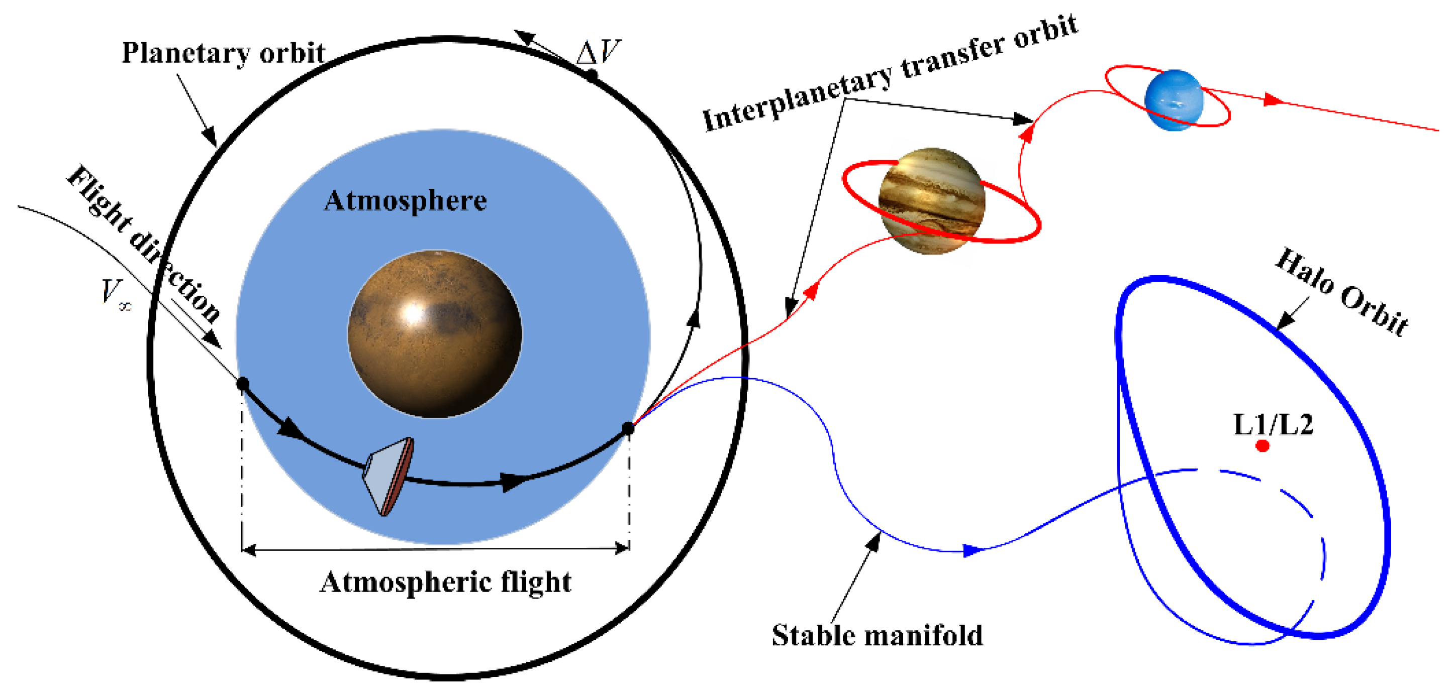
The high deceleration efficiency of aerocapture maneuver renders a wide range of potential applications. Typical applications are shown schematically in Figure 1. An aerocapture maneuver can capture a vehicle in a planetary orbit or deliver the vehicle into the periodic orbits around the Sun-planet libration points, such as collinear libration points 1 and 2 (L1 and L2) [9,10,11,12,13,14,15,16]. In addition, an aerocapture maneuver can adjust the phase and flight velocity of an interplanetary probe to fly along an ideal trajectory. Such an aerocapture mode is called aerogravity assist (AGA) [17,18,19]. Note that in both cases, the target orbit is eventually reached after aerocapture through an intermediate transfer orbit, such as the stable manifold of a halo orbit or an interplanetary transfer orbit. These transfer orbits are determined directly by the terminal state of the atmospheric flight. Therefore, accurately constructing the aerocapture attainability sets is crucial in assessing the vehicle’s reachable ability after aerocapture.

An aerocapture attainability set describes the maneuverability of the aerocapture and determines the feasibility of a given aerocapture mission. Constructing the aerocapture attainability set is equivalent to determining the boundary of the attainability set, and numerically solving the aerocapture trajectory for each terminal state on the boundary is a family of optimal control problems. Therefore, a robust and efficient algorithm of aerocapture trajectory planning is key to accurately construct and formulate the complete aerocapture attainability set.

To solve the aerocapture trajectory planning problem, many guidance algorithms have been proposed since the 1980s, such as the Apollo entry guidance scheme [20], analytic aerocapture guidance [21,22,23,24], and numerical predictive-corrector aerocapture guidance [25,26,27,28,29]. They are reliable but not globally optimal. At the same time, open-loop aerocapture trajectory optimization methods were also investigated [30,31,32,33]. In comparison with the guidance algorithms, optimization methods ensure the optimal characteristic of aerocapture trajectories. The aerocapture trajectory can be optimized by an indirect or direct method, such as the direct collocation pseudospectral method [34]. However, the open-loop optimization is slow in computation speed and has a worse convergence [35,36]. Consequently, existing aerocapture trajectory planning methods, both the guidance algorithms and the open-loop optimization methods, are not suitable for the rapid and accurate construction of an aerocapture attainability set.

This paper develops a robust and efficient algorithm based on convex optimization. Convex optimization is a popular method for rapid planning and has been used widely in aerospace in recent years. Typical applications include planetary powered descent guidance [37,38], space rendezvous and proximity operations [39], planetary entry trajectory planning [40], and path planning for zero-propellant maneuvers [41,42]. If a nonlinear programming problem can be formulated to a specific form of convex optimization, such as linear programming, second-order cone programming, and semidefinite programming [43], the optimal solution of the nonlinear problem can be found rapidly and accurately [44].

In Section 2, the aerocapture attainability set is defined in the longitudinal dynamics model, and the problem is formulated as determining the boundary of the attainability set. In order to obtain a complete point set, the boundary of the attainability set is discretized as a series of points by means of dimensionality reduction as in Section 3, and these boundary points are solved by our proposed convex method in Section 4. To adopt convex optimization, the original problem, which is highly nonlinear and nonconvex, is converted into a sequence of convex subproblems. Then, the solution of the original problem is approximated successively. Section 5 presents high-fidelity numerical results to demonstrate the robustness and efficiency of the proposed method. Finally, conclusions are drawn in Section 6.

2. Formulation of Aerocapture Attainability Set

The main phase of an aerocapture process is the planetary atmospheric flight. For an unpowered atmospheric flight, regardless of the transversal modulation and modeling in the nonrotating planet frame, the vehicle state at any time t during the aerocapture is defined as x(t) = [r, V, γ]^T, where r, V, and γ are the radial distance, velocity, and flight-path angle, respectively. The motion of the vehicle is described by the nondimensional dynamic differential equations [28]

$$\frac{dr}{dt}=V\sin \gamma$$

(1)

$$\frac{dV}{dt}=-D-\frac{\sin \gamma }{r^2}$$

(2)

$$\frac{d\gamma }{dt}=\frac{L\cos \sigma }{V}+(\frac{V^2}{r}-\frac{1}{r^2})\frac{\cos \gamma }{V}\hspace{0.17em}$$

(3)

The radial distance r is normalized by the radius of planet R_M, the relative velocity V is normalized by $\sqrt{{\mu }_M/R_M}$, and the nondimensional time t is normalized by $\sqrt{R_M^3/{\mu }_M}$, where µ_M is the gravitational parameter of the planet. The bank angle σ is the only control variable. The lift and drag acceleration L and D are normalized by $g_M={\mu }_M/R_M^2$,

$$\{\begin{array}{c}L=0.5\rho V^2{R}_{M}S{C}_L/m\\ D=0.5\rho V^2{R}_{M}S{C}_D/m\end{array}$$

(4)

where m represents the mass of the vehicle, S indicates the dimensional reference area, C_L and C_D represent the lift coefficient and drag coefficient, respectively, and $\rho ={\rho }_0\exp \left(-R_{M}h/h_s\right)$ is the dimensional atmospheric density, in which ρ₀ is the dimensional atmospheric density at R_M, h_s is the atmospheric density coefficient, and h is the nondimensional altitude.

Given the initial entry state of the atmospheric flight $\mathit{x}(t_0)=[r_0,V_0,{\gamma }_0]$, all the terminal states of the atmospheric flight form the attainability set of the aerocapture,

$$\mathcal{A}=\left\{{\mathit{x}}^i(t_f)|\mathit{x}(t_0)\right\},$$

(5)

where ${\mathit{x}}_i\left(t_f\right)={[r_f^i,V_f^i,{\gamma }_f^i]}^T$ is the terminal state of the i-th atmospheric flight trajectory. Note that as the height of atmosphere h_atm is usually a constant for a given planet, both r₀ and r_f are constant and equal to the radius of atmosphere r_atm, which is the height of atmosphere plus the radius of planet R_M. The terminal states are then distinguished only by $V_f$ and ${\gamma }_f$. Additionally, note that as an infinite small change in bank angle σ leads to a sufficiently small difference in terminal state, the aerocapture attainability set $\mathcal{A}$ is a simply connected region in the $V_f-{\gamma }_f$ space. An illustration of an aerocapture attainability set is shown in Figure 2, where the boundary of the attainability set is denoted as $\mathcal{O}$.

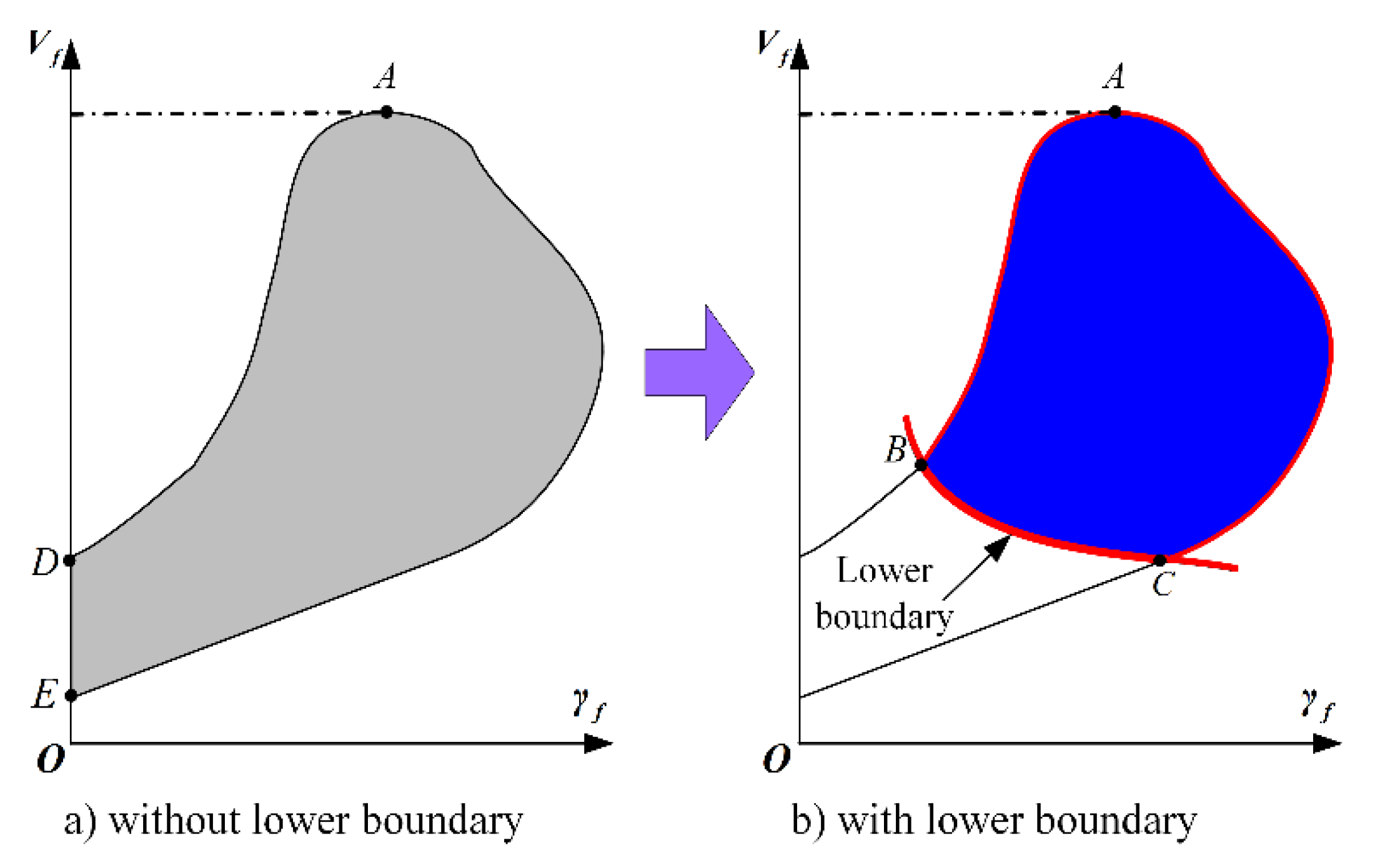
In this paper, the attainability set consists of only the terminal states of the vehicle exiting the atmosphere after aerocapture. If the vehicle drops into the atmosphere and eventually collides with the planet, the terminal state is excluded from the attainability set because the aerocapture failed. The demarcation of a successful and a failed aerocapture is ${\gamma }_f=0$, which is delineated by the line D-E in Figure 3a. Given that the target orbit after aerocapture is far from the atmosphere, a minimum altitude of periapsis $h_{a,\min }>h_{atm}$ is also constrained. Given the terminal state $\mathit{x}(t_f)$ of atmospheric flight, the constrain can be derived from the general energy equation of the elliptical orbit [28],

$$\frac{V_f^2}{2}-\frac{{\mu }_M}{r_{atm}}+\frac{{\mu }_M}{2}\left(\frac{2}{r_{a,\min }}-\frac{r_{atm}^2{V}_f^2{\cos }^2{\gamma }_f}{{\mu }_M{r}^2{}_{a,\min }}\right)=0$$

(6)

where $r_{a,\min }=h_{a,\min }+R_M$ is the radial distance of periapsis. This constraint imposes a lower boundary ${\mathcal{O}}_L$ on $\mathcal{A}$, as represented by the curve B-C in Figure 3b. As a summary, the boundary of the aerocapture attainability set ${\mathcal{O}}_L$ is the closed curve A-B-C as in Figure 3b.

3. Algorithm to Construct Aerocapture Attainability Set

Based on the formulation in Section 2, the aerocapture attainability set $\mathcal{A}$ can be constructed by determining its boundary $\mathcal{O}$. In this paper, the boundary is calculated by means of dimensionality reduction, as illustrated in Figure 4. The key idea is to determine the reachable bounds of ${\gamma }_f$ for each fixed $V_f$. For a specific $V_f^k$, the line $V=V_f^k$ intersects the boundary $\mathcal{O}$ at two points, denoted as ${\gamma }_{f,\min }^k$ and ${\gamma }_{f,\max }^k$. These two points are the solutions of the optimal control problems

$$\begin{array}{l}\underset{\sigma }{\min }{\gamma }_f\hspace{0.17em}\hspace{0.17em}\hspace{0.17em}\hspace{0.17em}\iff \hspace{0.17em}\hspace{0.17em}\hspace{0.17em}\hspace{0.17em}{\gamma }_{f,\min }^k\\ \underset{\sigma }{\max }{\gamma }_f\hspace{0.17em}\hspace{0.17em}\hspace{0.17em}\hspace{0.17em}\iff \hspace{0.17em}\hspace{0.17em}\hspace{0.17em}\hspace{0.17em}{\gamma }_{f,\max }^k\end{array}$$

(7)

subject to the given initial state x₀, where the state vector x = [r, V, γ]^T and the control variable σ follow the dynamic differential equations given in Equations (2)–(4). For convenience, the two problems are denoted as Problem 1.

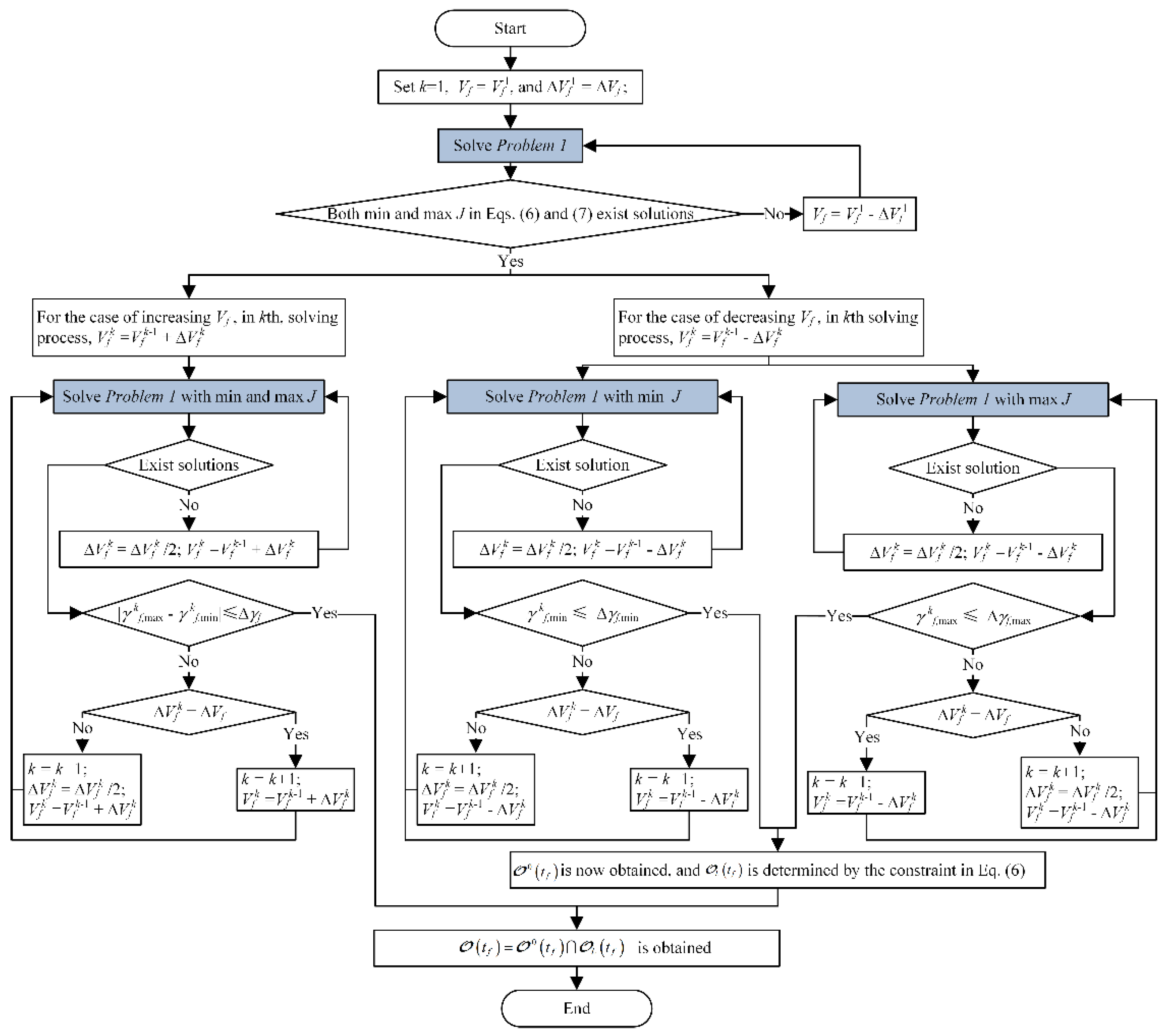
The algorithm flowchart for numerically solving the boundary $\mathcal{O}$ is summarized in Figure 5. Firstly, an initial terminal velocity $V_f^1$ is chosen where both the problems of min ${\gamma }_f$ and max ${\gamma }_f$ have solutions. Without loss of generality, $V_f^1$ can be set in accordance with the energy equation [45,46,47]

$$V_f^1=\sqrt{\frac{2{\mu }_M}{r_{atm}}-\frac{{\mu }_M}{r_a^R+r_p^R}}$$

(8)

where $r_a^R$ and $r_p^R$ are the apoapsis and periapsis radii of the estimated terminal orbit.

Then, the fixed terminal velocity is monotonically increased, $V_f^k=V_f^{k-1}+\Delta V_f^k$ with an adaptive step $\Delta V_f^k$, starting from $V_f^1$. With the stopping criterion

$$\left|{\gamma }_{f,\max }^k-{\gamma }_{f,\min }^k\right|\le \Delta {\gamma }_f$$

(9)

where $\Delta {\gamma }_f>0$ is a constant close to zero and the two reachable bounds of ${\gamma }_f$ eventually shrink into a common point A.

Next, the terminal velocity is monotonically decreased, $V_f^k=V_f^{k-1}-\Delta V_f^k$, starting from $V_f^1$. As the two reachable bounds of ${\gamma }_f$ do not shrink to a common point, ${\gamma }_{f,\min }^k\le {\gamma }_f^B$ and ${\gamma }_{f,\max }^k\le {\gamma }_f^C$ are adopted as the stopping criterions, where ${\gamma }_f^B$ and ${\gamma }_f^C$ are the flight-path angles at points B and C determined by Equation (6), respectively.

Note that the choice of step $\Delta V_f^k$ is crucial for the numerical determination of the boundary $\mathcal{O}$. In order to solve ${\gamma }_{f,\min }^k$ and ${\gamma }_{f,\max }^k$ precisely near the point A in the case of increasing $V_f$, and to avoid the vehicle crashing on the planet surface in the case of decreasing $V_f$, the step size $|\Delta V_f|$ should be reduced adaptively.

4. Solving with Sequential Convex Programming

Solving Problem 1 is an essential step in the algorithm, which is marked in Figure 5 with shaded blocks. Key procedures in solving Problem 1 such as convexification, discretization, and successive iteration are introduced in this section.

As the dynamic equations are nonlinear, Problem 1 is a highly nonlinear optimal control problem. To solve it using convex optimization, all the nonconvex items in Problem 1 need to be first converted into convex functions, resulting in a sequence of convex subproblems to approximate the solution of the original Problem 1. Such a method is called sequential convex programming. Note that the subproblems are not equivalent to the original nonlinear problem. As a result, successive approximation is then used until the solution of the convex subproblems is sufficiently close to the solution of the original problem.

4.1. Change of the Independent Variable

Because the boundary points are solved for each fixed terminal velocity $V_f$, it is convenient to use a new independent variable directly related to the velocity V to replace the time variable t in the original dynamic differential equations. In this paper, the nondimensional energy $e=1/r-V^2/2$ is chosen as the new independent variable. According to [48], $de/dt=DV>0$, indicating that e increases monotonically. Then, the nondimensional velocity can be computed inversely by $V=\sqrt{2/r-2e}$. During the solving process, it can be approximated by $V^{Z+1}=\sqrt{2/r^Z-2e}$ in the (z + 1)-th iteration of the successive approximation.

Replacing the time t by the new independent variable e, the original dynamic differential Equations (1)–(3) become

$$\frac{dr}{de}=\sin \gamma /D$$

(10)

$$\frac{d\gamma }{de}=\frac{L\cos \sigma }{V^{2}D}+(\frac{V^2}{r}-\frac{1}{r^2})\frac{\cos \gamma }{V^{2}D}$$

(11)

Note that using e as the independent variable can also simplify the dynamics. One differential equation is eliminated. The state vector then becomes $\mathit{x}={[r,\gamma ]}^T$.

4.2. New Control Variable

The bank angle σ is the only control variable which has lower and upper bounds on the magnitude

$${\sigma }_{\min }\le \left|\sigma \right|\le {\sigma }_{\max }$$

(12)

where ${\sigma }_{\min }$ is greater than 0 deg and ${\sigma }_{\max }$ must be less than 180 deg, because flying at a bank angle of 0 deg or 180 deg will cause the vehicle to have no crossrange control ability [28]. The bank angle is in the form of sine in the dynamic equations, which impedes the convergence of the optimal control problem. To overcome this issue, $u=\cos \sigma$ is defined as the new control variable. Then the constraint becomes

$$u_{\min }\le u\le u_{\max }$$

(13)

where $u_{\min }=\cos {\sigma }_{\max }$ and $u_{\max }=\cos {\sigma }_{\min }$. The constraint on u is naturally convex.

4.3. Successive Linearization for Dynamic Equations

The dynamics in Equations (10) and (11) are highly nonlinear. In order to convert Problem 1 into a convex subproblem, the dynamics should be linearized. Firstly, Equations (10) and (11) are rewritten into a concise form as:

$$\dot{\mathit{x}}={\mathit{f}}_0\left(\mathit{x},e\right)+\mathit{B}\left(\mathit{x},e\right)\cdot u$$

(14)

where $\dot{\mathit{x}}$ is the derivative of $\mathit{x}={[r,\gamma ]}^T$ with respects to e, the column vector

$${\mathit{f}}_0\left(\mathit{x},e\right)=\left[\begin{array}{c}\sin \gamma /D\\ \cos \gamma /\left(rD\right)-\cos \gamma /\left(r^2{V}^{2}D\right)\end{array}\right]$$

(15)

and the coefficient vector of the control variable

$$\mathit{B}\left(\mathit{x},e\right)={\left[\begin{array}{cc}0,& \left(L/D\right)/V^2\end{array}\right]}^T$$

(16)

For simplicity, the argument e is dropped in the remainder of this paper. The nonlinear dynamics in Equation (14) can be approximated by a successive small-disturbance-based linearization method [40]. Given an existing solution ${\mathit{x}}^z$ from the z-th iteration of the successive approximation process, the dynamic Equation (14) is linearized at ${\mathit{x}}^z$ in the (z + 1)-th iteration as

$$\dot{\mathit{x}}=\mathit{A}\left({\mathit{x}}^z\right)\mathit{x}+\mathit{B}\left({\mathit{x}}^z\right)\cdot u+{\mathit{f}}_0\left({\mathit{x}}^z\right)-\mathit{A}\left({\mathit{x}}^z\right){\mathit{x}}^z$$

(17)

where the coefficient matrix of the state vector

$$\mathit{A}\left({\mathit{x}}^z\right)=\frac{\partial {\mathit{f}}_0\left(\mathit{x}\right)}{\partial \mathit{x}}|\begin{array}{c}\\ \mathit{x}={\mathit{x}}^z\end{array}=\left[\begin{array}{cc}{a}_{11}& a_{12}\\ a_{21}& a_{22}\end{array}\right]$$

(18)

in which

$$\begin{array}{l}{a}_{11}=-\frac{D_r^Z\sin {\gamma }^Z}{{(D^Z)}^2},\\ a_{12}=\frac{\cos {\gamma }^Z}{D^Z},\\ a_{21}=\frac{(r^Z{D}_r^Z+D^Z)[1-r^Z{(V^Z)}^2]\cos {\gamma }^Z+D^Z\cos {\gamma }^Z}{{(r^Z)}^3{(D^Z)}^2{(V^Z)}^2},\\ a_{22}=\frac{[1-r^Z{(V^Z)}^2]\sin {\gamma }^Z}{{(r^Z)}^2{D}^Z{(V^Z)}^2}\end{array}$$

where

$$D_r^Z=\frac{\partial D}{\partial z}{|}_{x=x^z}=-\frac{R_M{D}^z}{h_S}$$

(19)

To ensure the validity of linearization, a trust–region constraint is used,

$$\left|\mathit{x}-{\mathit{x}}^z\right|\le \delta$$

(20)

where δ is the constrained boundary and set in accordance with the magnitudes of the elements in x.

4.4. Convex Subproblem

Linearizing Equation (14) into Equation (17), the original optimal control problem can be iteratively solved by a sequence of convex subproblems,

$$\underset{u}{\min }\mathrm{or}\underset{u}{\max }{\gamma }_f,$$

(21)

$$\mathrm{subject} \mathrm{to} \stackrel{·}{\mathit{x}}=A({\mathit{x}}^z)\mathit{x}+B({\mathit{x}}^z)-A({\mathit{x}}^z){\mathit{x}}^z$$

(22)

$$u_{\min }\le u\le u_{\max }$$

(23)

$$r(e_f)=r_{atm}$$

(24)

$$|\mathit{x}-{\mathit{x}}^z|\le \delta$$

(25)

which is denoted as Problem 2. The criterion of convergence is defined as

$$\underset{e_0\le e\le e_f}{\sup }|{\mathit{x}}^{z+1}(e)-{\mathit{x}}^z(e)|\le \epsilon ,$$

(26)

where ε is a constant vector, which represents the accuracy of the solution with respect to the original Problem 1.

4.5. Discretization

To solve Problem 2 numerically, the independent variable e is equally discretized into N + 1 points in the interval $[e_0,e_f]$. The constraints in Equations (23) and (25) apply for each of these points. The state vector and control variable are denoted as ${\mathit{x}}_i$ and ${\mathit{u}}_i$ for the i-th point, respectively. The variable sets $\left\{{\mathit{x}}_i\right\}$ and $\left\{u_i\right\}$ are the variables to be solved. The dynamic Equation (22) becomes

$${\mathit{x}}_{i+1}={\mathit{x}}_i+\frac{\Delta e}{2}[{\mathit{A}}_i^z{\mathit{x}}_i+{\mathit{B}}_i\cdot u_i+{\mathit{f}}_{0,i}^z-{\mathit{A}}_i^z{\mathit{x}}_i^z+{\mathit{A}}_{i+1}^z{\mathit{x}}_{i+1}+{\mathit{B}}_{i+1}^z\cdot u_{i+1}+{\mathit{f}}_{0,i+1}^z-{\mathit{A}}_{i+1}^z{\mathit{x}}_{i+1}^z]$$

(27)

where i = 0, 1, ⋯, N − 1 and $\Delta e=(e_f-e_0)/N$. After rearrangement, Equation (27) is then rewritten into

$$\left(\mathit{I}+\frac{\Delta e}{2}{\mathit{A}}_i^z\right){\mathit{x}}_i+\left(\frac{\Delta e}{2}{\mathit{A}}_{i+1}^z-\mathit{I}\right){\mathit{x}}_{i+1}+\frac{\Delta e}{2}{\mathit{B}}_i^z{u}_i+\frac{\Delta e}{2}{\mathit{B}}_{i+1}^z{u}_{i+1}+\frac{\Delta e}{2}\left({\mathit{b}}_i^z+{\mathit{b}}_{i+1}^z\right)=0$$

(28)

where I is a unit matrix with the same dimension as ${\mathit{A}}_i^z$ and ${\mathit{b}}_i^z={\mathit{f}}_{0,i}^z-{\mathit{A}}_i^z{\mathit{x}}_i^z$.

The discretized problem is denoted as Problem 3, which is equivalent to and has the same solution as Problem 2. The performance index is given by Equation (21). The linear equality constraints are given by Equations (24) and (28). The linear inequality constraint is given by Equation (25).

4.6. Procedure of Iteration

The successive procedure to solve Problem 1 is summarized as follows:

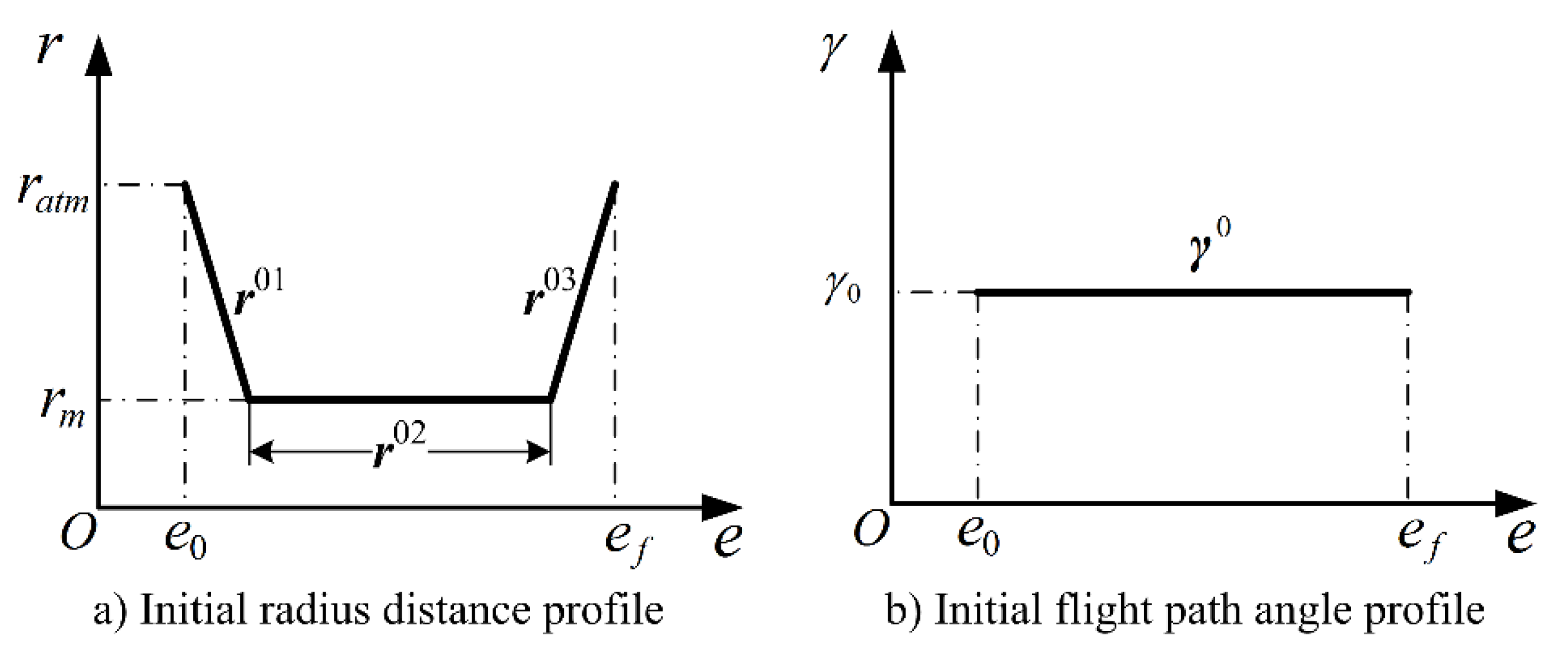
Step 1: Set z = 0 and the state vectors $\left\{{\mathit{x}}_i^0\right\}$ to an initial profile. In accordance with the trajectory characteristic of a normal aerocapture flight, the initial profile of radial distances is given as $\left\{r^{01} r^{02} r^{03}\right\}$, as shown in Figure 6a. $r^{01}$ is a straight line from $r_{atm}$ to $r_m=1+h_{atm}/2$ divided evenly as $[N/10]$ points, $r^{02}$ is a straight line from $r_m$ to $r_m$ having $N+1-2[N/10]$ points, and $r^{03}$ is a straight line from $r_m$ to $r_{atm}$ having $[N/10]$ points. The symbol [ ] is the floor function mapping a real number onto the largest integer that is less than or equal to the real number. The initial flight-path angle profile is chosen as a constant value ${\gamma }_0$ as shown in Figure 6b. Note that choosing the initial guess is not necessary because the solution of the convex optimization problem is unique. However, a good initial profile can accelerate the convergence of the numerical procedure.

Step 2: The solution of the z-th iteration ${\mathit{x}}^z$ is chosen to be the initial profile in the (z + 1)-th iteration to solve ${\mathit{x}}^{z+1}$ and $u^{z+1}$ [49,50].

Step 3: Check the convergence criterion

$$\underset{0\le i\le N}{\max }\left|{\mathit{x}}_i^{z+1}\left(e\right)-{\mathit{x}}_i^z\left(e\right)\right|\le \epsilon$$

(29)

If it is satisfied, then proceed to step (4); otherwise, go to step (2) for the next iteration.

Step 4: The solution of Problem 1 is found to be ${\mathit{x}}^{\ast }={\mathit{x}}^{z+1}$ and $u^{\ast }=u^{z+1}$.

It is worth to note that approximating by a sequence of convex optimizations as in Problem 3, although the convergence of sequential approximation to the original Problem 1 remains to be proven, a considerable number of preceding studies have provided sufficient confidence in the convergence [37,38,39,40,41,42,43]. In this paper, the numerical simulations of solving the aerocapture attainability sets given in Section 5 showed good performance and reliability of the developed convex method.

In general, aiming at the convergence of the method proposed in this paper, it can mainly be improved in three aspects. First, the dynamic model reduces the state quantity by one dimension through the substitution of independent variables, thereby reducing the complexity of the problem. Secondly, the groove-shaped initial trajectory is given for the solution of boundary points for the first time calculation, which increases the feasibility of the problem. Finally, when solving other boundary points, the initial value is given by the optimal solution of the previous solution. This adjacency idea greatly improves the sensitivity of the initial value.

5. Numerical Demonstrations

As Mars is a hot destination for deep space exploration, the Mars aerocapture was taken as an example to verify our proposed algorithm. The radius of Mars is R_M = 3396 km. The gravitational parameter of Mars is µ_M = 42,828 km³/s². The Orion Multi-Purpose Crew Vehicle (MPCV) [28] was used in our simulations. The mass of the Orion MPCV is 10,387 kg. The spacecraft always flies a trim angle-of-attack profile and the hypersonic lift–drag ratio L/D is 0.27. The lift and drag coefficients are C_D = 1.37 and C_L = 0.37, respectively. The reference area of the vehicle is 19.86 m². The initial states entering the atmosphere of Mars are listed in

Table 1. Initial conditions of Mars aerocapture.

States	h0, km	V0, m/s	γ0, deg
Values	128	5900	−11

[3].

In the construction of the aerocapture attainability set, the lower boundary given in Equation (6) was applied with a minimum altitude of apoapsis $h_{a,\min }$ = 200 km after the atmospheric flight. The terminal orbit was estimated with the size of 300 × 3000 km to initialize the terminal velocity in Equation (8). The initial adaptive step of terminal velocity was ${\Delta }_f^1$ = 100 m/s. The stopping criterions were $\Delta {\gamma }_f$ = $\Delta {\gamma }_{f,\min }$ = ${\gamma }_{f,\max }^k$ = 0.01 deg.

In the solving of optimal control problems, the lower and upper bounds of the bank angle in Equation (12) were set to be ${\sigma }_{\min }$ =15 deg and ${\sigma }_{\max }$ = 165 deg, respectively. For the case of D ≤ 0.1 g_M, the states were integrated directly with zero bank angle because of the weak modulation of the vehicle in the thin atmosphere. The trust-region boundary in Equation (25) was $\delta ={[6000/R_M,\pi /4]}^T$. The stopping criterion of successive approximation in Equation (29) was $\epsilon ={[200/R_M,0.05\pi /180]}^T$. The problem was discretized by N = 300 and solved by the state-of-the-art primal-dual interior point method (PDIPM), which is efficient and accurate in solving convex programming problems without initial guess [51] using the mature software MOSEK [52]. All computations were performed via MATLAB-R2018a on a desktop with Intel i7-4790K CPU @4.00 GHz.

In addition, various simulations with different initial states and parameters of the vehicle were also investigated to determine the impact of different parameters on the constructed aerocapture attainability set.

5.1. Geometric Structure of the Aerocapture Attainability Sets

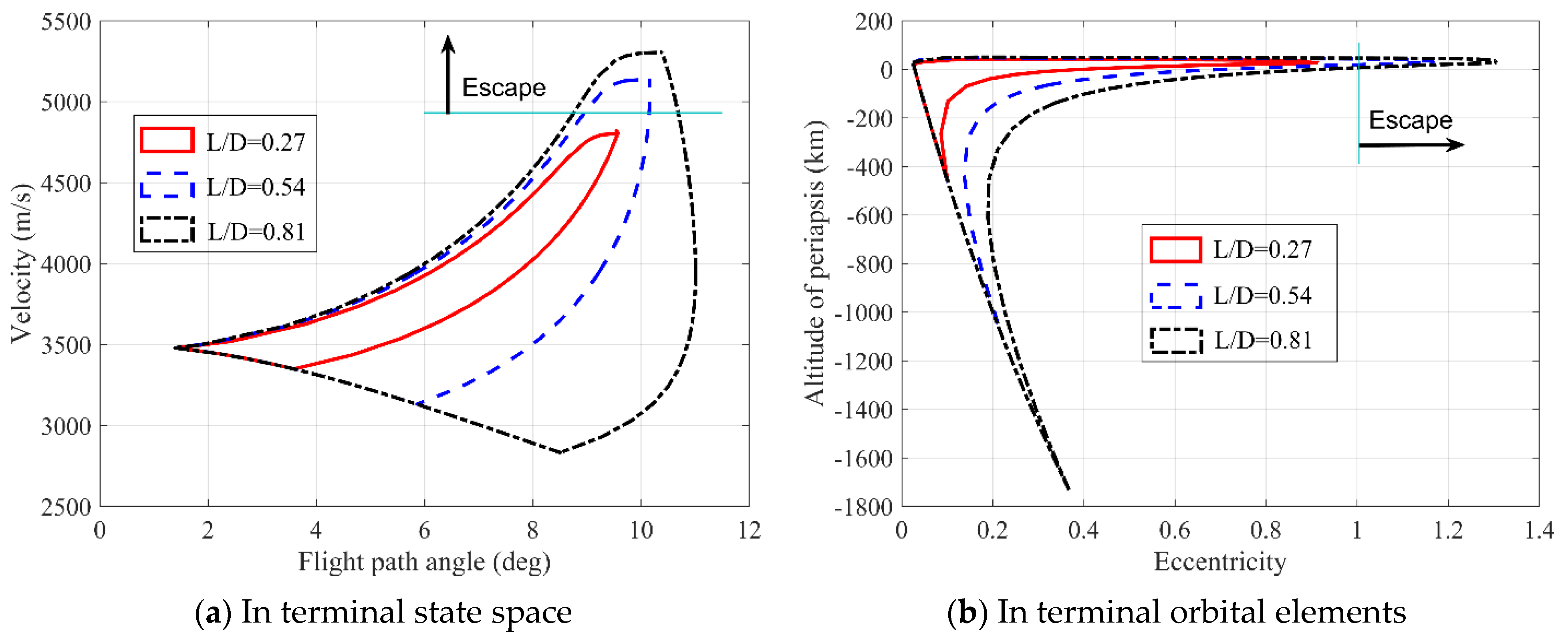
Figure 7a shows the aerocapture attainability set for the initial state given in Table 1, plotted in the state space. The flight-path angle has a wide range for a low terminal velocity. As the terminal velocity increases, the boundary of the attainability set eventually shrinks to point A. Without a lower boundary limit given by Equation (6), the attainability set extends infinitely close to ${\gamma }_f=0$ and even to ${\gamma }_f\le 0$, where the vehicle falls into the atmosphere. The corresponding orbit elements are plotted in Figure 7b. The eccentricity of the terminal orbit is calculated using Keplerian orbital mechanics [28],

$$e_f=\sqrt{\frac{a_f-V_f^2{r}_{atm}^2{\cos }^2{\gamma }_f}{a_f}}$$

(30)

The nondimensional semimajor axis is $a_f=1/(2/r_{atm}-V_f^2)$, and the periapsis of the terminal orbit has a nondimensional altitude $h_{p,f}=a_f(1-e_f)-1$. As shown in the figure, the larger the terminal flight-path angle, the larger the eccentricity of the terminal orbit. Besides, the left boundary of the attainability set, the curve A-B in Figure 7a, gives a stable upper boundary of the altitude of periapsis, the curve A1-B1 in Figure 7b.

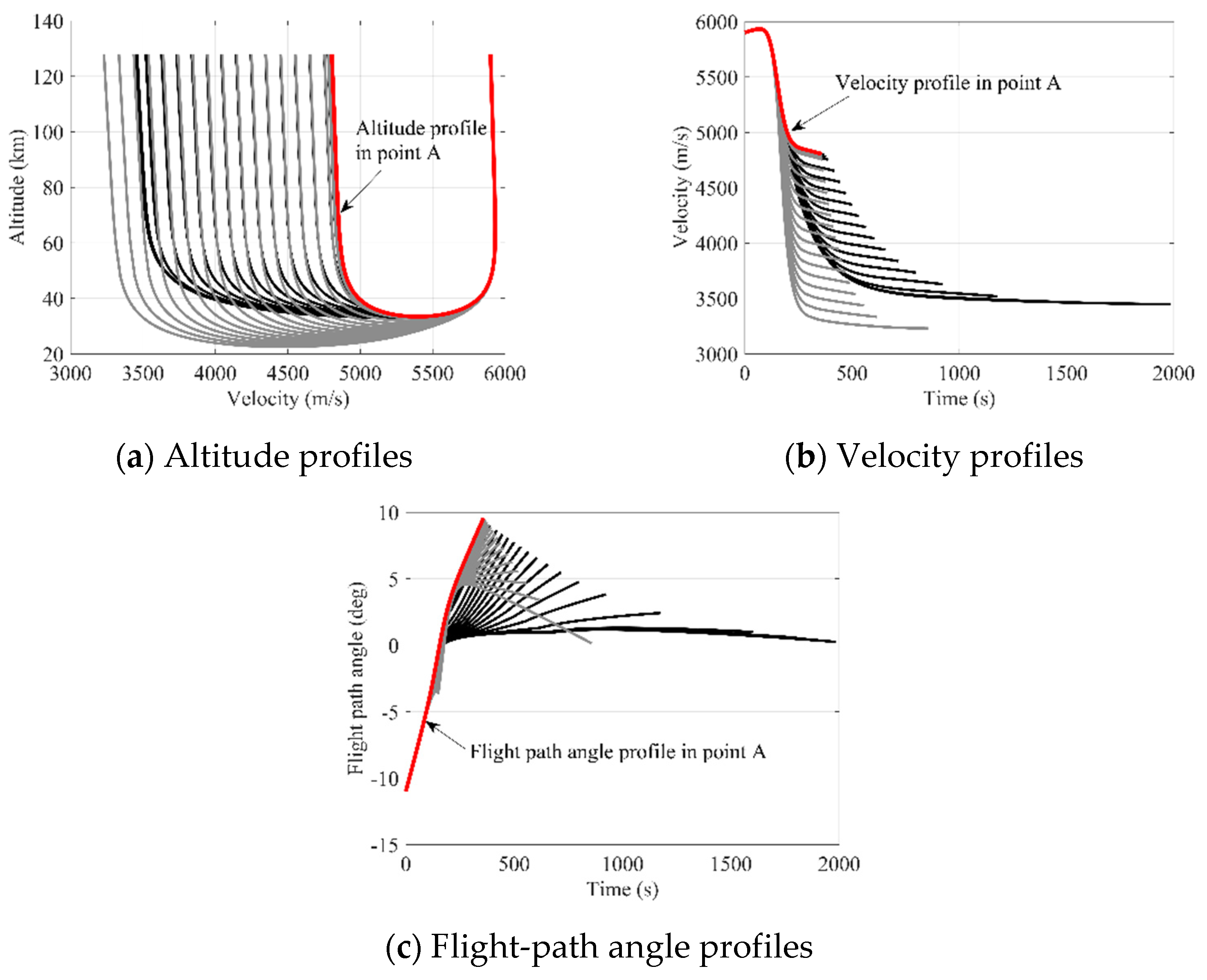
The altitude, velocity, and flight-path angle profiles are shown in Figure 8. The state profiles plotted with black and grey colors have terminal states on the left and right boundaries of the attainability set in Figure 7a, respectively, and the state profiles corresponding to the point A are highlighted with the red color. Figure 8a shows that the atmospheric flights with a terminal state on the right boundary of the attainability set have a lower flight altitude in the atmosphere than those on the left boundary. They require a larger change in flight-path angle, and the vehicle must fly at a lower altitude to obtain enough lift to increase $d\gamma /dt$. Figure 8b shows that the time of atmospheric flight for a terminal state on the left boundary of the attainability set is longer than that on the right boundary. Meanwhile, Figure 8c indicates that the flight-path angle for a terminal state on the left boundary changes more smoothly during the atmospheric ascent phase than that on the right boundary.

Note that, in the aforementioned computing environment, it took a total of 7.47 s to calculate the envelope of the attainability set in Figure 7. Specifically, a total of 57 extreme values of points were calculated, and the average calculation time per extreme value was about 0.131 s. That is, it took only about a hundred milliseconds. At the same time, in the process of solving all extreme values, the successive approximation was generally completed between 4~7 steps, and the calculation time of each step was about 0.02~0.03 s, which is equivalent to the time of solving a convex subproblem. The statistical results of the calculation time demonstrate the high efficiency of the proposed method, and it also verifies the feasibility of the method to determine the aerocapture attainability set onboard for an aerocapture mission.

5.2. Aerocapture Attainability Sets with Different Initial Velocity

Figure 9 shows the aerocapture attainability sets with different initial velocities $V_0$ = 5.6, 5.9 and 6.2 km/s. A large $V_0$ increases the range of the attainability set to a higher terminal velocity and flight-path angle. The terminal states in the subset of the attainability set, separated by the cyan line, makes the vehicle escape from the planet. This subset provides the possibility of delivering the vehicle into a periodic orbit around the Sun-planet L1 or L2 points, which renders a fuel-efficient interplanetary transfer.

5.3. Aerocapture Attainability Sets with Different Initial Flight-Path Angles

The initial flight-path angle ${\gamma }_0$ is also an important design parameter for aerocapture. For Mars aerocapture, the permissible range of ${\gamma }_0$ is relatively small. Three different initial flight-path angles ${\gamma }_0$= −10.5 deg, −11.0 deg, and −11.5 deg were considered in our simulations. The resulting attainability sets are shown in Figure 10. The larger the initial flight-path angle, the larger the aerocapture attainability set expanded to a higher terminal velocity and flight-path angle.

5.4. Aerocapture Attainability Sets with Different Hypersonic Lift–Drag Ratios

Although the lift–drag ratios are fixed for the Orion MPCV, the analysis of the aerocapture attainability set with different hypersonic lift–drag ratios can provide some knowledge of the vehicle’s structure design. In our simulations, C_D is fixed as 1.37, and C_L varies with different lift–drag ratios L/D. As shown in Figure 11, the hypersonic lift–drag ratio has a significant impact on the range of the aerocapture attainability set. A higher lift–drag ratio results in a larger attainability set. Additionally, the aerocapture attainability set with a high lift–drag ratio contains the ones with lower lift–drag ratios. In our simulations, ${\mathcal{A}}_{L/D=0.27}\subset {\mathcal{A}}_{L/D=0.54}\subset {\mathcal{A}}_{L/D=0.81}$.

5.5. Aerocapture Attainability Sets with Different Upper Bounds of Bank Angle

For the optimal aerocapture process, the optimal bank angle profile has a bang-bang control structure. Hence, the bank angle switches between σ_min to σ_max. Thus, the bounds of the bank angle are significantly related to the crossrange control ability [28]. In our simulation, the lower bound of the bank angle is fixed, and the aerocapture attainability set influence was analyzed with different upper bounds of bank angle σ_max. As shown in Figure 12, the attainability sets are similar with σ_max = 125 deg, 165 deg, but for σ_max = 85 deg, the aerocapture attainability set significantly contracted. It shows that σ_max < 90 deg greatly weakens the longitudinal control ability of the vehicle during the atmospheric flight.

5.6. Influence of Path Constraints to the Aerocapture Attainability Sets

Heating rate, load factor, and dynamic pressure [53]

$$\dot{Q}=9.4369\times {10}^{-9}{\left(\sqrt{g_M{R}_M}\right)}^{3.15}\sqrt{\rho }{V}^{3.15}\le {\dot{Q}}_{\max }$$

(31)

$$n=\sqrt{L^2+D^2}\le n_{\max }$$

(32)

$$q=0.5\times {10}^{-3}{g}_M{R}_M\rho V^2\le q_{\max }$$

(33)

are important path constraints during the atmospheric flight. The heating rate $\dot{Q}$ of the stagnation point on the surface of the vehicle is in watts per square centimeter. The load factor n is in $g_M$. The dynamic pressure q is in kilonewtons per square meter. The unit of dimensional atmospheric density ρ is in kilograms per cubic meter, and the velocity V is nondimensional. Correspondingly, ${\dot{Q}}_{\max }$, $n_{\max }$, and $q_{\max }$ are the upper limits of the heating rate, load factor, and dynamic pressure limits, respectively. Given that $V=\sqrt{2/r^z-2e}$, the constraints are rewritten in the form of radial distance as

$$r\left(e\right)\ge r_{\dot{Q}}\left(e\right)=\frac{-2h_s}{R_M}\ln \frac{{\dot{Q}}_{\max }}{9.4369\times {10}^{-9}{\left(\sqrt{g_M{R}_M}\right)}^{3.15}\sqrt{{\rho }_0}{V}^{3.15}}+1$$

(34)

$$r\left(e\right)\ge r_n\left(e\right)=-\frac{h_s}{R_M}\ln \frac{2m{n}_{\max }}{R_{M}S\sqrt{C_L{}^2+C_D{}^2}{\rho }_0{V}^2}+1$$

(35)

$$r\left(e\right)\ge r_q\left(e\right)=-\frac{h_s}{R_M}\ln \frac{2\times {10}^3{q}_{\max }}{g_M{R}_M{\rho }_0{V}^2}+1$$

(36)

where $r_{\dot{Q}}\left(e\right)$, $r_n\left(e\right)$, and $r_q\left(e\right)$ are the minimum allowed radial distances for a given e corresponding to the upper limits of heating rate, load factor, and dynamic pressure, respectively. These path constraints are linear inequality constraints and must be all satisfied in the solving of Problem 1 with convex optimization.

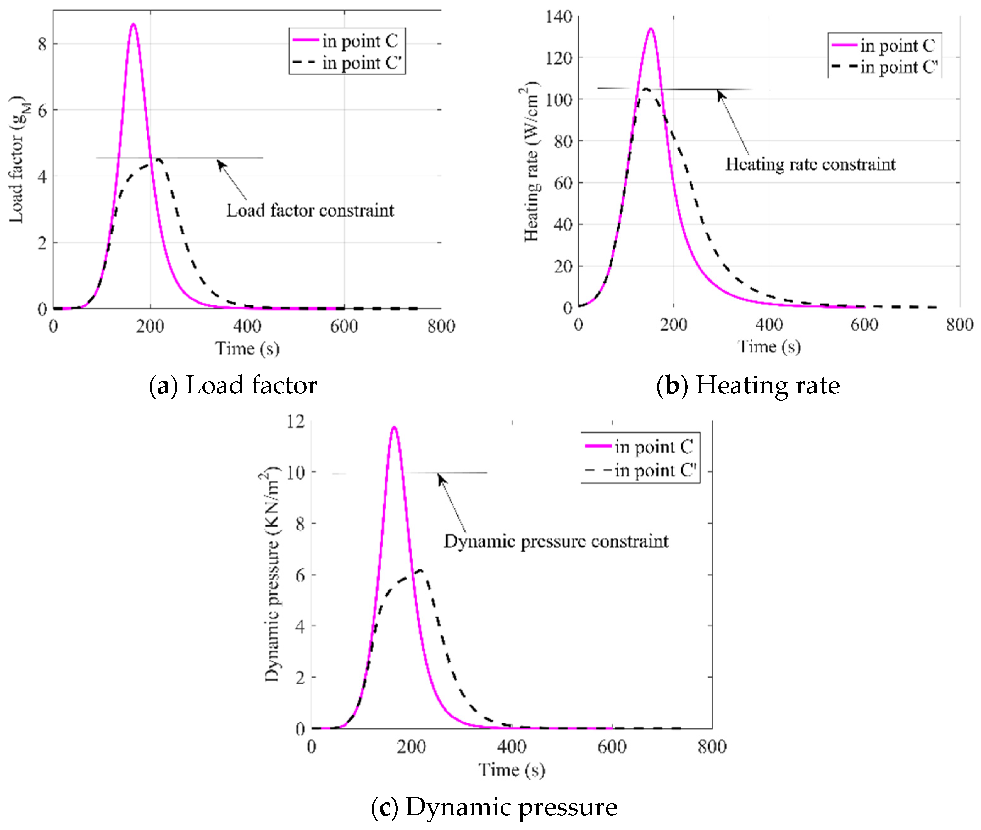
The path constraints in the simulation were ${\dot{Q}}_{\max }$ = 105 W/cm², $n_{\max }$ = 4.5 $g_M$, and $q_{\max }$ = 10 KN/m². Note that the upper boundary of the path constraint usually depends on the corresponding endurance of the spacecraft. For a low lift-to-drag ratio spacecraft, the heating rate constraint is generally between 30 and 300 W/cm², and the maximum overload peak value does not exceed 20 g_M. The path constraint boundary values used in this paper refer to the design values of most existing Mars rovers. The resulting aerocapture attainability sets with and without path constraints are plotted in Figure 13. It shows that path constraints significantly reduce the range of the aerocapture attainability set.

The peak load factor, heating rate, and dynamic pressure together with the atmospheric flight time of aerocapture for each of the points A, B, C and C′ are given in

Table 2. The peak load factor, heating rate, and dynamic pressure together with the atmospheric flight time of aerocapture for each of the points A, B, C and C′ in Figure 13.

Point	$\mathbf{Max} \dot{\mathit{Q}}$, W/cm2	Max n, gM	Max q, KN/m2	Flight Time, s
A	126.973	6.602	9.036	437.86
B	104.946	3.682	5.040	1576.59
C	133.893	8.585	11.750	602.011
C’	105.000	4.500	6.159	753.59

. The bank angle profiles of the four characteristic points are shown in Figure 14. Despite the case of D ≤ 0.1 $g_M$, wherein the states are integrated directly with a zero bank angle, the bank angle in the optimal profile switches twice, and the ${\sigma }_{\max }$ always appears in the middle arc. In point C’, a singular arc of the bank angle profile exists, that is, the bank angle profile is not exactly the bang-bang control structure used to satisfy the path constraints. The comparison of the path variable profiles between points C and C’ is shown in Figure 15, which intuitively reflects the effect of suppressing the path variables. Generally, large peak values of the path variables may threaten the aerocapture vehicle; however, the results in this subsection indicate that the peak values of the path variables are tolerable for Mars aerocapture.

6. Conclusions

In this paper, an algorithm was proposed to determine the exact aerocapture attainability set on the basis of convex optimization. The efficiency and robustness of the proposed algorithm were demonstrated successfully by a variety of examples. To solve the aerocapture attainability set, its boundary was converted into a set of points by means of dimensionality reduction. Finding each element in the point set was an optimal control problem and was achieved by using the convex method.

The simulation showed the aerocapture attainability set was affected by the following parameters: the initial velocity, the initial flight-path angle, the lift–drag ratio, and the maximum magnitude of the bank angle. Moreover, among these parameters, L/D had the greatest effect on the aerocapture attainability set; a larger $V_0$ can expand the aerocapture attainability and increase the capability of the aerocapture flight, whereas a smaller σ_max, such as less than 90 deg, can greatly weaken the longitudinal control ability of the vehicle during the atmospheric flight. Moreover, the influence of path constraints on aerocapture attainability sets was simulated. It revealed that the existence of path constraints reduces significantly the range of aerocapture attainability sets.

Numerical simulations showed the proposed method works well during the solving process. Because of the relatively low computational cost, the proposed algorithm can potentially be used onboard to rapidly assess the aerocapture attainability set.

Aiming at the problem of solving the general aerocapture attainability set, in order to further improve the online computing capability, future work should focus on how to analytically characterize the structure of the attainability set and how to switch a point-by-point solution to a characterization parameter calculation.

References

- Craig, S.; Lyne, J.E. Parametric study of aerocapture for missions to Venus. J. Spacecr. Rocket. 2005, 42, 1035–1038. [Google Scholar] [CrossRef]
- Han, H.; Qiao, D.; Chen, H. Optimal ballistic coefficient control for Mars aerocapture. In Proceedings of the 2016 IEEE Chinese Guidance, Navigation and Control Conference (CGNCC), Nanjing, China, 12–14 August 2016; pp. 2175–2180. [Google Scholar]
- Hamel, J.F.; de Lafontaine, J. Improvement to the analytical predictor-corrector guidance algorithm applied to Mars aerocapture. J. Guid. Control Dyn. 2006, 29, 1019–1022. [Google Scholar] [CrossRef]
- Meyer, J.L.; Silverberg, L.; Walberg, G.D. Fuel-optimal bank-angle control for lunar-return aerocapture. J. Spacecr. Rocket. 1995, 32, 149–155. [Google Scholar] [CrossRef]
- Putnam, Z.R.; Braun, R.D. Drag-modulation flight-control system options for planetary aerocapture. J. Spacecr. Rocket. 2014, 51, 139–150. [Google Scholar] [CrossRef]
- Aso, S.; Yasaka, T.; Hirayama, H.; Poetro, R.E.; Hatta, S. Preliminary studies on the planetary entry to Jupiter by aerocapture technique. Acta Astronaut. 2006, 59, 651–660. [Google Scholar] [CrossRef]
- Han, H.; Qiao, D. Optimization for the aeroassisted orbital plane change with the synergetic maneuver using the hp-adaptive pseudospectral method. J. Aerosp. Eng. 2017, 30, 04017076. [Google Scholar] [CrossRef]
- Kozynchenko, A.I. Development of optimal and robust predictive guidance technique for Mars aerocapture. Aerosp. Sci. Technol. 2013, 30, 150–162. [Google Scholar] [CrossRef]
- Li, X.; Qiao, D.; Macdonald, M. Energy-saving capture at Mars via backward stable orbits. J. Guid. Control Dyn. 2019, 42, 1136–1145. [Google Scholar] [CrossRef]
- Farquhar, R.W.; Dunham, D.W.; Guo, Y.; McAdams, J.V. Utilization of libration points for human exploration in the Sun–Earth–Moon system and beyond. Acta Astronaut. 2004, 55, 687–700. [Google Scholar] [CrossRef]
- Qi, Y.; Qiao, D. Angular momentum analysis in the elliptic restricted three-body problem. Mon. Not. R. Astron. Soc. 2022, 512, 5535–5545. [Google Scholar] [CrossRef]
- Li, X.; Qiao, D.; Christian, C. Mars high orbit capture using manifolds in the sun–mars system. J. Guid. Control Dyn. 2020, 43, 1383–1392. [Google Scholar] [CrossRef]
- Nakamiya, M.; Scheeres, D.J.; Yamakawa, H.; Yoshikawa, M. Analysis of capture trajectories into periodic orbits about libration points. J. Guid. Control Dyn. 2008, 31, 1344–1351. [Google Scholar] [CrossRef] [Green Version]
- Wang, Y.; Qiao, D.; Cui, P. Analysis of two-impulse capture trajectories into halo orbits of Sun-Mars system. J. Guid. Control Dyn. 2014, 37, 985–990. [Google Scholar] [CrossRef]
- Qi, Y.; Qiao, D. Stability analysis of Earth co-orbital objects. Astron. J. 2022, 163, 211. [Google Scholar] [CrossRef]
- Shahid, K.; Kumar, K.D. Nonlinear station-keeping control in the vicinity of the sun-earth l2 point using solar radiation pressure. J. Aerosp. Eng. 2016, 29, 04015073. [Google Scholar] [CrossRef]
- Armellin, R.; Lavagna, M.; Ercoli-Finzi, A. Aero-gravity assist maneuvers: Controlled dynamics modeling and optimization. In Periodic, Quasi-Periodic and Chaotic Motions in Celestial Mechanics: Theory and Applications; Springer: Berlin/Heidelberg, Germany, 2006; pp. 391–405. [Google Scholar]
- Mazzaracchio, A. Flight-path angle guidance for aerogravity-assist maneuvers on hyperbolic trajectories. J. Guid. Control Dyn. 2015, 38, 238–248. [Google Scholar] [CrossRef]
- Edelman, P.J.; Longuski, J.M. Optimal aerogravity-assist trajectories minimizing total heat load. J. Guid. Control Dyn. 2017, 40, 2699–2703. [Google Scholar] [CrossRef]
- Stiles, J. Predictive entry guidance for an Apollo-type vehicle. In Proceedings of the 3rd International IFAC Conference on Automatic Control in Space, Toulouse, France, 2–6 March 1970; Volume 3, pp. 732–740. [Google Scholar]
- Miele, A. The 1st John V. Breakwell Memorial Lecture: Recent advances in the optimization and guidance of aeroassisted orbital transfers. Acta Astronaut. 1996, 38, 747–768. [Google Scholar] [CrossRef]
- Gamble, J.D.; Cerimele, C.J.; Moore, T.E.; Higgins, J. Atmospheric guidance concepts for an aeroassist flight experiment. J. Astronaut. Sci. 1988, 36, 45–71. [Google Scholar]
- Masciarelli, J.; Rousseau, S.; Fraysse, H.; Perot, E. An analytic aerocapture guidance algorithm for the Mars Sample Return Orbiter. In Proceedings of the Atmospheric Flight Mechanics Conference, Denver, CO, USA, 14–17 August 2000. [Google Scholar]
- Graves, C.; Masciarelli, J. An analytical assessment of aerocapture guidance and navigation flight demonstration for applicability to other planets. In Proceedings of the AIAA Atmospheric Flight Mechanics Conference and Exhibit, Boston, MA, USA, 19–22 August 2013. [Google Scholar]
- Liang, Z.; Li, Q.; Ren, Z. Virtual terminal–based adaptive predictor–corrector entry guidance. J. Aerosp. Eng. 2017, 30, 04017013. [Google Scholar] [CrossRef]
- Starr, B.; Westhelle, C. Aerocapture Performance analysis of a Venus explorer mission. In Proceedings of the AIAA Atmospheric Flight Mechanics Conference and Exhibit, San Francisco, CA, USA, 15–18 August 2005. [Google Scholar]
- Jits, R.Y.; Walberg, G.D. Blended control, predictor–corrector guidance algorithm: An enabling technology for Mars aerocapture. Acta Astronaut. 2004, 54, 385–398. [Google Scholar] [CrossRef]
- Lu, P.; Cerimele, C.J.; Tigges, M.A.; Matz, D.A. Optimal aerocapture guidance. J. Guid. Control Dyn. 2015, 38, 553–565. [Google Scholar] [CrossRef]
- Masciarelli, J.; Westhelle, C.; Graves, C. Aerocapture guidance performance for the neptune orbiter. In Proceedings of the AIAA Atmospheric Flight Mechanics Conference and Exhibit, Providence, RI, USA, 16–19 August 2004. [Google Scholar]
- Wetzel, T.A.; Moerder, D.D. Vehicle/trajectory optimization for aerocapture at Mars. J. Astronaut. Sci. 1994, 42, 71–89. [Google Scholar]
- Sigal, E.; Guelman, M. Optimal aerocapture with minimum total heat load. In Proceedings of the 52nd International Astronautical Congress, Toulouse, France, 1–5 October 2001. [Google Scholar]
- Armellin, R.; Lavagna, M. Multidisciplinary optimization of aerocapture maneuvers. J. Artif. Evol. Appl. 2008, 2008, 248798. [Google Scholar] [CrossRef] [Green Version]
- Knittel, J.; Lewis, M. Multidisciplinary optimization of starbody waverider shapes for lifting aerocapture with orbital plane change. In Proceedings of the 18th AIAA/3AF International Space Planes and Hypersonic Systems and Technologies Conference, Tours, France, 24–28 September 2012. [Google Scholar]
- Patterson, M.A.; Rao, A.V. Exploiting sparsity in direct collocation pseudospectral methods for solving optimal control problems. J. Spacecr. Rocket. 2012, 49, 354–377. [Google Scholar] [CrossRef]
- Miele, A.; Wang, T.; Lee, W.Y. Optimization and guidance of trajectories for coplanar, aeroassisted orbital transfer. J. Astronaut. Sci. 1990, 38, 311–333. [Google Scholar]
- Chai, R.; Savvaris, A.; Tsourdos, A.; Chai, S.; Xia, Y. Unified multiobjective optimization scheme for aeroassisted vehicle trajectory planning. J. Guid. Control Dyn. 2018, 41, 1521–1530. [Google Scholar] [CrossRef]
- Acikmese, B.; Ploen, S.R. Convex programming approach to powered descent guidance for Mars landing. J. Guid. Control Dyn. 2007, 30, 1353–1366. [Google Scholar] [CrossRef]
- Blackmore, L.; Açikme¸se, B.; Scharf, D.P. Minimum-landing-error powered-descent guidance for Mars landing using convex optimization. J. Guid. Control Dyn. 2010, 33, 1161–1171. [Google Scholar] [CrossRef] [Green Version]
- Lu, P.; Liu, X. Autonomous trajectory planning for rendezvous and proximity operations by conic optimization. J. Guid. Control Dyn. 2013, 36, 375–389. [Google Scholar] [CrossRef]
- Liu, X.; Shen, Z.; Lu, P. Entry trajectory optimization by second-order cone programming. J. Guid. Control Dyn. 2016, 39, 227–241. [Google Scholar] [CrossRef]
- Zhang, S.; Friswell, M.I.; Wagg, D.J.; Tang, G.J. Rapid path planning for zero-propellant maneuvers. J. Aerosp. Eng. 2016, 29, 04015078. [Google Scholar] [CrossRef]
- Zhang, S.; Zhao, Q.; Huang, H.B.; Tang, G.J. Rapid path planning for zero propellant maneuvers based on flatness. J. Aerosp. Eng. 2017, 30, 04017054. [Google Scholar] [CrossRef]
- Liu, X.; Lu, P.; Pan, B. Survey of convex optimization for aerospace applications. Astrodynamics 2017, 1, 23–40. [Google Scholar] [CrossRef]
- Chen, Q.; Qiao, D.; Wen, C. Minimum-Fuel low-thrust trajectory optimization via reachability analysis and convex programming. J. Guid. Control Dyn. 2021, 44, 1036–1043. [Google Scholar] [CrossRef]
- Pan, B.; Lu, P.; Chen, Z. Coast arcs in optimal multiburn orbital transfers. J. Guid. Control Dyn. 2012, 35, 451–461. [Google Scholar] [CrossRef]
- Pan, B.; Lu, P.; Pan, X.; Ma, Y. Double-homotopy method for solving optimal control problems. J. Guid. Control Dyn. 2016, 39, 1706–1720. [Google Scholar] [CrossRef]
- Luo, Y.Z.; Sun, Z.J. Safe rendezvous scenario design for geostationary satellites with collocation constraints. Astrodynamics 2017, 1, 71–83. [Google Scholar] [CrossRef]
- Lu, P. Entry Guidance: A unified method. J. Guid. Control Dyn. 2014, 37, 713–728. [Google Scholar] [CrossRef]
- Wen, C.; Zhao, Y.; Shi, P. Precise determination of reachable domain for spacecraft with single impulse. J. Guid. Control Dyn. 2014, 37, 1767–1779. [Google Scholar] [CrossRef]
- Wen, C.; Peng, C.; Gao, Y. Reachable domain for spacecraft with ellipsoidal delta-v distribution. Astrodynamics 2018, 2, 265–288. [Google Scholar] [CrossRef]
- Nesterov, Y.E.; Todd, M.J. Primal-Dual Interior-Point Methods for Self-Scaled Cones. SIAM J. Optim. 1998, 8, 324–364. [Google Scholar] [CrossRef]
- MOSEK, A. The MOSEK Optimization Toolbox for MATLAB Manual. Version 7.1 (Revision 28). 2015. Available online: http://docsmosekcom/71/toolbox/indexhtml (accessed on 29 May 2022).
- Han, H.; Qiao, D.; Chen, H.; Li, X. Rapid planning for aerocapture trajectory via convex optimization. Aerosp. Sci. Technol. 2019, 84, 763–775. [Google Scholar] [CrossRef]
Figure 1.
Potential missions achieved by aerocapture.
Figure 2.
Illustration of the aerocapture attainability set in state space.
Figure 3.
The boundary of aerocapture attainability set in state space.
Figure 4.
Solving the boundary of aerocapture attainability set by dimensionality reduction.