Mixed-Flow Load-Balanced Scheduling for Software-Defined Networks in Intelligent Video Surveillance Cloud Data Center

Abstract

As the large amount of video surveillance data floods into cloud data center, achieving load balancing in a cloud network has become a challenging problem. Meanwhile, we hope the cloud data center maintains low latency, low consumption, and high throughput performance when transmitting massive amounts of data. OpenFlow enables a software-defined solution through programing to control the scheduling of data flow in the cloud data center. However, the existing scheduling algorithm of the data center cannot cope with the congestion of the network center effectively. Even for some dynamic scheduling algorithms, adjustments can only be made after congestion occurs. Hence, we propose a proactive and dynamically adjusted mixed-flow load-balanced scheduling (MFLBS) algorithm, which not only takes into account the different sizes of flows in the network but also maintains maximum throughput while balancing the load. In this paper, the MFLBS problem was formulated, along with a set of heuristic algorithms for real-time feedback and adjustment. Experiments with mesh and tree network models show that our MFLBS is significantly better than other dynamic scheduling algorithms, including one-hop DLBS and static scheduling algorithm FCFS. The MFLBS algorithm can effectively reduce the delay of small flows and average delay while maintaining high throughput.

1. Introduction

With the support of the internet of things (IoT) and cloud computing, new-generation information systems have gained increasing prominence in recent decades. Among them, intelligent video surveillance applications require massive computing and storage resources [1,2,3,4,5,6,7] to offer a high quality of service. However, the complexity of video surveillance task and the diversity of data in different dimensions, such as volume, variable, and velocity, inevitably cause a heavy burden on the network. Therefore, with a large amount of video surveillance data flooding to the cloud center, cloud data center networks are facing increasing data transmission problems [8]. At this time, the network throughput has become the bottleneck of video surveillance transmitting massive data. What needs to be solved urgently is the issue of traditional hardware devices and static scheduling algorithms finding it difficult to handle the transmission task for such massive amounts of information. The emergence of software-defined networking (SDN) [9] solves the problems of traditional hardware, which is non-programable. SDN uses methods including centralization of network control and separation of control logic and underlying switches, allowing researchers to use related technologies (OpenFlow [10]) to focus on the network flow scheduling algorithm to meet different needs.

One of the highly recognized schemes is load-balanced scheduling [11]. Load-balanced scheduling increases the network throughput and reduces the end-to-end delay of the flow by balancing the traffic transmitted on the network link. Dynamic load-balanced scheduling algorithms can better adapt to the real-time changing state of the network when compared with the inextensibility of traditional static scheduling algorithms [12]. Nowadays, some load-balanced scheduling algorithms have been proposed for data center networks [13,14]. Nevertheless, some of these algorithms only care about the overall throughput of the network and perform the same processing for all flows in the network [15]. Not specifically considering the characteristics of different flows results in high latency for small flows in some conditions. Furthermore, some of the dynamic adjustment algorithms rely on the corresponding feedback mechanism after the network is blocked. Therefore, the performance of the network is closely related to the selected corresponding threshold, which is a critical value defined by different articles to measure network performance [12]. A relatively low threshold will add extra overhead to the network, whereas a relatively high threshold will not significantly alleviate the network congestion. The algorithm is passive if it only adjusts when it meets the congestion threshold. In a word, the diversity and uncertainty of network tasks lead to more complex scientific problems. A single strategy cannot achieve the goal well, so a composite adaptive method is needed.

Inspired by the above situation, the MFLBS algorithm is designed to prevent network congestion through a proactive scheduling mechanism and dynamically adjusted on routing and bandwidth allocation in real time to maximize network throughput and reduce delay, according to the network situation. We split the entire network into two sub-nets: first, tune into the dynamic routing network of the flow to balance the network load and take into account the delay of the small flow, and then, enter the static routing network to actively prevent network congestion, according to the network status. Meanwhile, the MFLBS algorithm is tested in the widely used tree and mesh network topologies [16] to observe its universality. The specific contributions of this article are as follows:

• A new cloud data center scheduling algorithm (MFLBS) is proposed and formulated to achieve the goal of maximizing throughput.
• Considering the characteristics of both large and small flows, we integrate active congestion control and real-time dynamic scheduling methods, and originally divide the traditional network into two sub-nets, performing network transmission according to the characteristics of different streams and different stages of scheduling. The two sub-nets can adjust the bandwidth allocation ratio V(α) on each link according to different transmission tasks and topological structures.
• A heuristic algorithm is designed for the MFLBS problem and tested on two highly versatile network topologies: the partial mesh model and the three-layer non-blocking fully populated network model.
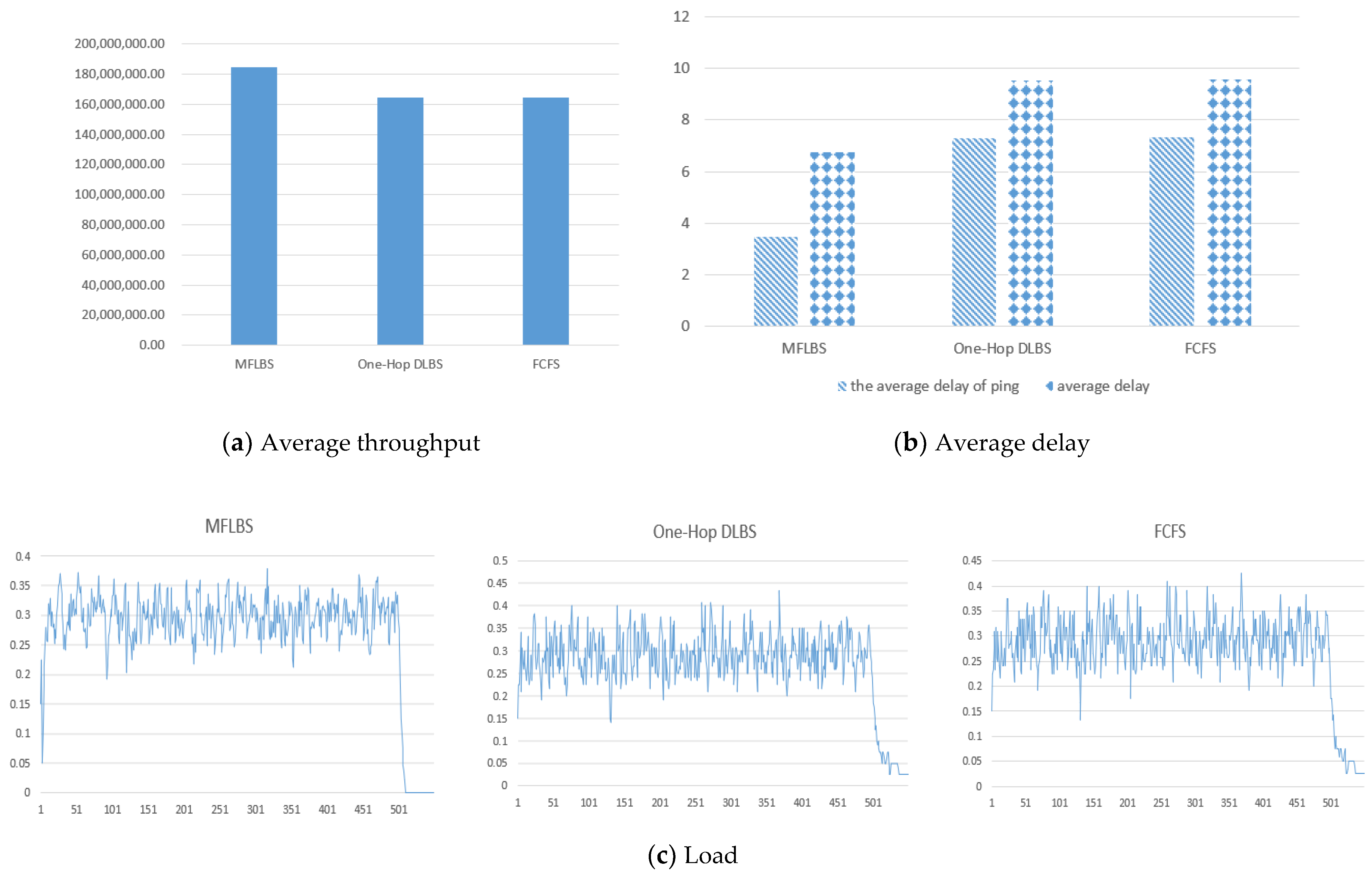
• A simulation experiment is designed for the cloud data center, and the MFLBS algorithm is compared with two other algorithms: the dynamic scheduling algorithm one-hop DLBS [17] and the static load-balanced scheduling algorithm FCFS [18]. The result proves that our algorithm can significantly improve the throughput and effectively reduce the average delay of the flow.

The remaining content of the article is as follows. Section 2 reviews related work, and Section 3 details the network model of the data center used in this article and formulates the MFLBS problem. The scheduling mechanism of the two sub-nets and our MFLBS algorithm is described in Section 4. Subsequently, designs of the simulations are put forward in Section 5 to test the MFLBS algorithm and compare the MFLBS algorithm with other scheduling algorithms. Finally, Section 6 includes the summary of our research and future work.

2. Related Work

Flow scheduling has always been a popular research direction in the network. In the following section, we will review the different research results obtained by the predecessors.

2.1. Flow Scheduling

Existing algorithms can be roughly divided into static scheduling and dynamic scheduling algorithms, according to whether they can feedback the network status in real time and perform corresponding adjustments. Static algorithms, such as the classic FCFS algorithm, have been developed and applied in different scenarios. J. P. Champati et al. studied the distribution of AOI in two-hop WNCS in Ref. [18] and devised a problem of minimizing the tail of the AoI distribution with respect to the frequency of generating information updates, i.e., the sampling rate of monitoring a process, under first-come-first-serve (FCFS) queuing discipline. The Baraat system designed by Dogar F R et al. [19], although based on the static scheduling algorithm FIFO, combined with the task-aware network, is a typical dynamic scheduling scheme.

With the diversification of transmission tasks and requirements, more and more researchers turn their attention to achieving superior performance through the innovation of transmission units. The author puts forward PRISM in Ref. [20], a fine-grained perception of the MapReduce scheduler, and divides it into stages to improve the resource utilization of Hadoop when the job is running. Y. Wang et al. [21] considered the budget and deadline of the MapReduce job and designed a task-level scheduling algorithm based on this constraint. Having successfully optimized a cost-effective budget through the greedy strategy, F. Carpio et al. proposed a new load-balancing solution: DiffFlow [22]. This is a mechanism to forward packets by distinguishing long and short streams and using random packet spraying (RPS) with the help of SDN. However, this situation will potentially lead to a disorderly arrival of data packets.

Moreover, researchers can also design algorithms with better performance by designing different underlying frameworks. Li and Xu [23] classified the load-balancing strategies in SDN based on different architectures. In the centralized architecture, a controller manages the connected network devices to concentrate the load-balancing work on the data plane. In the distributed architecture, multiple controllers are used to exchange and connect to each device, or studies such as Refs [24,25] improve their goals by using MPTCP from the perspective of network protocol.

In a word, researchers have explored different angles and methods to improve the performance of network transmission, and most of the mainstream research is based on OpenFlow.

2.2. OpenFlow-Based Schemes

As a popular technology in software-defined networking, OpenFlow is used by researchers as the basis to achieve more innovative integrations. F. Tang et al. [17] used the calculation of the link threshold congestion to perform global dynamic rerouting and transferred the largest flow from the link that exceeded the threshold. Therefore, two algorithms called DLBS are proposed to adapt to different tree structures. This method with load balancing as the goal improves the utilization of network bandwidth. X. Cao et al. introduced SDN/OpenFlow technology into the complex and difficult-to-control ops network and proposed an OF-OPS network structure combined with the OpenFlow control process. Through the perception of competition for tasks in the network, the routing/rerouting strategy is combined to distribute traffic under the premise of load balancing [26].

With the development of cloud computing, the problem of data center traffic transmission has also become a research hotspot. Hedera [27] is a representative centralized control scheduling system to dynamically manage the flow and effectively improve the utilization of resources. Chowdhury M. [28] proposed a data-intensive framework Varys, combining Coflows and effective heuristics (SEBF) to improve network utilization and ensure freedom of starvation. Ramos R. M. proposes SlickFlow [29], a flexible routing method based on OpenFlow for fast error recovery. This mechanism simplifies the forwarding task in the switch and can effectively recover from failures. In [30], considering that streaming media requires a lot of resources, R. Bhattacharyya et al. develop QFlow, a platform that standardizes this feedback loop and initiates a variety of control policies over it. The experiments on YouTube verify its high-quality service guarantee.

In summary, the existing algorithms based on flow scheduling cannot actively control network congestion. The static algorithm has insufficient scalability, only executing the scheduling algorithm at the beginning of the transmission, which cannot adapt well to the real-time changing network state. The existing dynamic load-balanced algorithms can provide adjustment locally or even globally, but they can only adjust a network that has reached the performance bottleneck after the fact, according to the feedback mechanism. A single strategy cannot achieve the goal well, so a composite adaptive method is needed. Our work focuses on dynamic load-balancing algorithms for proactive congestion control.

3. Network Model and Problem Statement

We firstly introduce two common network models used in our experiments and then formulate the mixed-flow load-balanced scheduling (MFLBS) problem.

3.1. Network Model

We model the cloud data center as an undirected graph G = <V, E>, where V is the collection of all switches $s$ and hosts $h$ in the network, and E is the collection of links connecting these switches and hosts. All links adopt a full-duplex communication mode, which means that data can be simultaneously transmitted on the same link.

Considering the actual application and the simulation of network performance, we adopt the following two models accepted by most researchers [31,32,33,34].

The first one is the network center model with three-tier architecture. h1~h8 are clients and nodes that generate data transmission tasks. s1~s10 are switches, forming a hierarchical inter-networking model with core layer, convergence layer, and access layer. This three-layer non-blocking fully populated network is at the center of today’s network. It has a wide range of applications [35], shown in Figure 1.

In the second type of network topology shown in Figure 2, we use a two-layer architecture, where S1~S9 are the core layer switches, and each switch has its own access layer and client. For example, S1 and its corresponding components are a group of networks; S11 and S12 are access layers; and h1~h4 are clients. In real life, this network topology covers fewer networks and ranges but reduces the workload of deployment and maintenance.

All the switches in this article support the OpenFlow protocol, which means that the packets in the flow have sequence numbers to record their position in the flow. If the flow changes the corresponding path during transmission, the packet will arrive at a random time node. However, there is no need to retransmit the packets that have been transmitted before; instead, after all the flows are transmitted, the packets are reordered according to the sequence number.

3.2. MFLBS Problem

The goal of MFLBS is to balance the traffic load of the data center through the use of sub-net division and a combination of dynamic and static mechanisms to maximize the throughput of the entire network.

Assuming that there are K flows $K=\left\{f_1,f_2,f_3\cdots \cdots f_k\right\}$ in a certain time slot $t_0$ in the network, then $a^{f_k}\left(t_0\right)$ represents the traffic transmitted from the source to the destination of a single flow $f_k$ in this time slot $t_0$. In other words, we divide the continuous time T into time slots $t\left(t=1,2,\dots ,T\right)$, and the total network transmission traffic can be expressed as ${\sum }_{t=1}^T{\sum }_{k=1}^K{a}^{f_k}(t)$. For any switch $i$, its outgoing traffic and incoming traffic are the same, that is, the traffic ${\sum }_{t=1}^T{\sum }_{k=1}^K{a}^{f_k}(t)$ from $i$ to the neighboring switch $s_i$ should be balanced with the traffic ${\sum }_{t=1}^T{\sum }_{k=1}^K{a}^{f_{k\ast }}(t)$ from the neighboring switch $s_i$ to this switch $i$. It is worth noting that $a^{f_k}$ here refers to the actual allocated bandwidth. Because it is limited by the actual network environment, its value may be different from the original required bandwidth.

To achieve network load balancing, we set up an ordered set for each single flow $f_k$, such as $f_k\left\{1,2\dots ,s\right\}$, to record its planned path. The values stored in the set are the numbers of the switches that pass through in the sequence during $f_k$ scheduling, and the ordered pair <i,j> are two adjacent elements in the ordered set. The orderly assembly of the path is adjusted according to the load situation of the network by adopting dynamic and static mechanisms.

The notations for the MFLBS problem formulation are listed in Notations.

Based on the above analysis, we first give the target formula of the MFLBS problem:

$$M\mathrm{ax}\frac{1}{T}{\sum }_{t=1}^T{\sum }_{k=1}^K{a}^{f_k}\left(t\right)$$

(1)

$${\sum }_{t=1}^T{\sum }_{k=1}^K{\alpha }_{i,j}^{f_k}\left(t\right)={\sum }_{t=1}^T{\sum }_{k\ast =1}^K{\alpha }_{j,i}^{f_{k\ast }}\left(t\right) i,j\in V\left(s\right)$$

(2)

$${\gamma }_{i,j}^{f_k}\left(t\right)\ge 0 i,j\in V\left(s\right)\cap E\left(f_k\right)$$

(3)

$${\sum }_{k=1}^K{\alpha }_{i,j}^{f_k}\le C_{i,j}{\gamma }_{i,j}^{f_k}\left(t\right)\ge {\alpha }_{i,j}^{f_k}\left(t\right)<i,j>\in V\left(s\right)\cap E\left(f_k\right)$$

(4)

$${\gamma }_{i,j}^{f_k}\left(t\right)\ge {\alpha }_{i,j}^{f_k}\left(t\right)i,j\in V\left(s\right)\cap E\left(f_k\right)$$

(5)

Equation (1) shows that the optimization direction of the MFLBS problem is to maximize the average throughput of the network. The left side of the equal sign in Equation (2) represents the sum of the outgoing traffic of all switches in the network; the right side of the formula represents the incoming traffic; and V(S) is the set of switches, which means that the incoming and outgoing bandwidth needs to be balanced for the entire network. Equation (3) indicates that the required bandwidth for any flow in the survival time slot must be a positive number. Equation (4) ensures that the sum of the actual bandwidth allocated on any link cannot exceed the total bandwidth of its own. Equation (5) reveals that the actual allocated bandwidth may be less than the bandwidth requested by the client under the influence of the network environment; if the network is not overloaded, it is equal.

4. Mixed-Flow Load-Balanced Scheduling (MFLBS)

In this section, we introduce our own MFLBS method, which roughly consists of two stages: when a flow arrives in the network, it first enters (1) the dynamic routing network for scheduling, and then, the flow that meets some conditions enters (2) the static routing network for transmission until the end. (1) The dynamic routing network and (2) static routing network will be shown in Section 4.1 and Section 4.2, respectively. Section 4.3 will explain which flows will be selected into the static routing network and the relationship between the bandwidth allocation in the two networks.

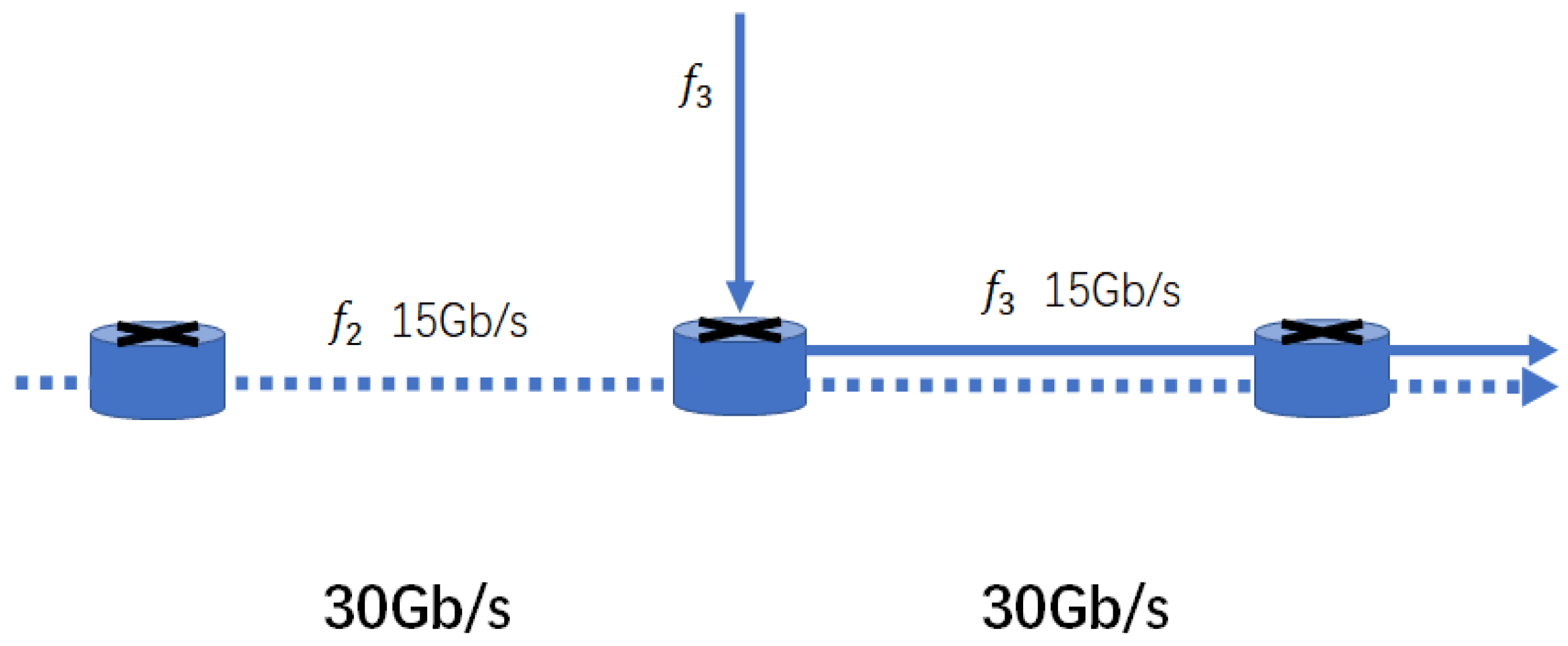
4.1. Dynamic Routing Network

According to the literature, most of the flows in data centers are short flows [36]. Although they account for a small part of the total amount of data transmitted in the network, unreasonable scheduling will cause great delays to these flows, which will further cause congestion and affect network performance. In view of the suddenness and unpredictability of the network, we treat all network flows as short flows at the beginning, which must be scheduled by the dynamic routing network. Section 4.1.1 and Section 4.1.2, respectively, introduce the method of initial path and rerouting, and Section 4.1.2 gives the Algorithm 1 for the flow in a single time slot to enter the dynamic routing network.

4.1.1. Initial Path Selection

Data centers have different requirements for stream transmission services. We adopt the highest weight first served (HWFS) strategy to assign the corresponding priority $p^{f_k}$ to the newly arrived stream $f_k$ in the network, and then, the switch will execute the tasks in descending order according to the priority of the flow in the queue. We use Dijkstra’s algorithm to determine the best initial path of $f_k$ according to the current network utilization state to make full use of the free bandwidth in the network and achieve the purpose of load balancing. It is worth noting that the priority of each stream is not fixed and can be modified according to the deadline, service requirements, network state, etc., but the priority determined in the current time slot is used for routing selection.

4.1.2. Dynamic Routing Mechanism

In each time slot, the switch will transmit data according to the priority. If the bandwidth on the initial path in this time slot has been allocated, $f_k$ will wait until the higher-priority flow transmission task in the queue ends, and the excess bandwidth is left before its transmission can be started.

This situation seriously affects the performance of the network and will further aggravate the local congestion of the network. Therefore, we need to reroute the paths of these flows. First, we need to maintain two tables (

Table 1. Remaining bandwidth table.

Links	Remaining Available Bandwidth
	t = 1	t = 2	t = 3	…
S1→S5	300	280	132	…
S1→S6	300	300	240	…
S1→S7	300	120	54	…
S1→S8	300	84	84	…
S2→S5	300	210	260	…
S2→S6	300	140	20	…
…	…	…	…	…

. Remaining bandwidth table and

Table 2. Maximum flow allocation table.

Links	The Flow Allocation with Max Bandwidth
	t = 1	t = 2	t = 3	…
S1→S5	f1	f2	f2	…
S1→S6	f2	f1	f1	…
S1→S7	f4	f4	f6	…
S1→S8	f5	f8	f8	…
S2→S5	f9	f9	f9	…
S2→S6	f7	f10	f10	…
…	…	…	…	…

. Maximum flow allocation table) to obtain global information and update the contents of the table in real time during the scheduling process. The remaining bandwidth table records the unallocated traffic on the path between the two shortest connection switches, and the maximum allocated flow table records the current flow allocated to the most traffic on the shortest link.

Then, we schedule in order of the priority and query the remaining bandwidth table, in turn, according to each link of the initial path of the flow $f_k$. If the remaining traffic on the corresponding link in the table is less than the required bandwidth ${\gamma }^{f_k}$ of $f_k$, mark the flow of the maximum allocated bandwidth that has been obtained on this link and update the final actual bandwidth $a^{f_k}$ of $f_k$.

Algorithm 1. Dynamic Routing Network Scheduling

Input: remaining bandwidth and maximum allocation flow table

Output: load-balanced scheduling

E ← the route of the marked flow in Maximum allocation flow table;

2. R ← the set of remaining allocatable bandwidth on the link in Remaining bandwidth table;

3. update E;

4. reset R;

5. new flows arrive on the network;

6. K ← total number of flows on the network;

7. arrange all flows in the network in descending order of priority: $f_1$, $f_2$,…$f_k;$

8. for k 1 to K by 1, do

9.    route based on R for unrouted flows;

10.  find the remaining bandwidth on the path, mb ← the minimum value of the remaining bandwidth on the path;

11.   if (mb ≥ ${\gamma }^{f_k}\left(t\right)$)

12.    $a^{f_k}\left(t\right)\leftarrow {\gamma }^{f_k}\left(t\right)$, allocate the required bandwidth to $f_k$;

13.   else

14.    mb ← ${\gamma }^{f_k}\left(t\right)$, allocate the maximum allocatable bandwidth on the link to $f_k$;

15.  mark the flow corresponding to the first link that does not meet the required bandwidth in E;

16.  update E and R;

17. end.

Finally, we determine the new route for these marked flows according to the network state and the Dijkstra algorithm in the next time slot. In the following section, we outline the important steps of dynamic routing network scheduling in a time slot.

4.2. Static Routing Network

As the data flow and network status change from time to time, in the dynamic routing network, there may be a situation in which the flow $f_k$ occupies a large bandwidth ratio of the link, or the transmission duration is too long, causing the routing times to increase continuously. This will increase the extra network overhead and waste resources considerably. For the flow from the dynamic network to the static network, we fix the path and adjust the bandwidth allocation to achieve the goal of optimizing the average throughput. In Section 4.2.1, we introduce the method of bandwidth allocation between different flows, and Section 4.2.2 introduces the calculation of the bottleneck bandwidth of the flow $f_k$ in detail. Therefore, we provide the Algorithm 2 for the static routing network in a time slot in Section 4.2.2.

4.2.1. Bandwidth Allocation

For different flows on the same link, we allocate bandwidth according to the max–min fairness algorithm. In order to avoid starvation caused by the delay in obtaining the corresponding bandwidth for the flow with low priority, some literature provides a method to adjust the priority to adapt to the new network conditions.

Here, we give the right to fair competition for bandwidth to all flows entering the static routing network.

$$p^{f_{k^{\prime }}}=p^{f_k}\hspace{1em}{k}^{\prime }=k\in (1,2,\dots ,K)\hspace{1em}\forall <i,j>\in f_k\{\dots \}\cap <i,j>\in f_{k^{\prime }}\{\dots \}$$

(6)

where, if the flow $f_k$ and flow $f_{k^{\prime }}$ have the same link segment in their respective routes, their priorities will be the same.

Therefore, the two newly arrived flows $f_k$ and $f_{k^{\prime }}$ on the same link $l_{i,j}$ in Figure 3 will equally divide the link bandwidth $C_{i,j}$ with the flow $f_1$ that originally exists on the link $l_{i,j}$. The three flows each obtain 10 Gb/s at this time, but the required bandwidth of $f_k$ 8 Gb/s is less than the obtained bandwidth 10 Gb/s, and the bandwidth obtained by $f_k$ and $f_1$ has not reached the corresponding required bandwidth 20 Gb/s, so the links $l_{i,j}$ will take back the excess 2 Gb/s of $f_k$ and distribute it equally to $f_{k^{\prime }}$ and $f_1$ again. Finally, $f_1$, $f_k$, and $f_{k^{\prime }}$ on $l_{i,j}$ obtain actual bandwidths of 11 Gb/s, 8 Gb/s, and 11 Gb/s, respectively.

4.2.2. Bottleneck Bandwidth Calculation

We all know that flows are subject to different restrictions on different link segments, and the bandwidth obtained on the most restricted link is the bottleneck bandwidth of this flow. For example, in Figure 4, $f_2$ shares bandwidth with $f_3$ on $l_{j,k}$, and exclusive bandwidth on links $l_{i,j}$, so the bottleneck bandwidth is the 15 Gb/s obtained on $l_{j,k}$.

The bottleneck bandwidth deeply affects the obtained bandwidth of the flow. We give the formulation $a^{f_k}$ = min(${\mathrm{e}}^{f_k}$, ${\gamma }^{f_k}$), that is, the obtained bandwidth takes the smaller value of the required bandwidth and the bottleneck bandwidth. In order to obtain $\mathrm{e}$, we need to calculate the restricted speed of the flow link by link, according to the route of the flow, and maintain an allocatable resource table to simulate the remaining network state after the bandwidth has been allocated. Two values are recorded on each link in the

Table 3. Allocatable resource table.

Links	Remaining Available Bandwidth and Unallocated Flow Numbers
	∅	f1	f7	…
S1→S5	6300	5180	5180	…
S1→S6	7300	7300	7300	…
S1→S7	3300	3300	3300	…
S1→S8	2300	2300	1210	…
S2→S5	5300	5300	5300	…
S2→S6	4300	4300	4300	…
…	…	…	…	…

: the number of flows with unallocated bandwidth ${l_{i,j}}^{\ast }\left(N\right)$ and the remaining bandwidth $B_{i,j}$. Different from the real-time recording of the remaining bandwidth table of the network status in the dynamic routing network, the allocatable resource table is used to calculate the bandwidth allocation of the flow in advance. Each time the actual allocated bandwidth of a flow is determined, the allocatable bandwidth table needs to be updated. Each time slot needs to maintain a new table.

We process the flows in ascending order according to the required bandwidth. First, we need to query the route E($f_k$) of the flow $f_k$. For a certain link$l_{i,j}$, $\langle i,j\rangle \in E\left(f_k\right)$ in the routing, we first assume that the flow does not restrict the flow on this link but normally performs the max–min fairness algorithm with other flows to allocate bandwidth. From this, we can calculate the limited bandwidth $E$ = $B_{i,j}/ {l_{i,j}}^{\ast }\left(N\right)$. We repeat the above calculations for the other link segments in E($f_k$) sequentially and finally obtain a set V(E). The smallest value in the set is the flow bottleneck bandwidth ${\mathrm{e}}^{f_k}$. Finally, we need to update the remaining bandwidth $B_{i,j}$ of the link segment passed by $f_k$ in the table according to the allocated bandwidth $a^{f_k}$ and reduce the value of ${l_{i,j}}^{\ast }\left(N\right)$ by one. Repeat the above process until the bandwidth of all flows in this time slot has been determined.

In the following algorithm, we outline the important steps of static routing network scheduling in a time slot.

Algorithm 2. Static Routing Network Scheduling

Input: allocatable resource table

Output: load-balanced scheduling

new flows arrive on the network;

2. R ← the set of remaining allocatable bandwidth on the link in Allocatable resource table;

3. k ← unallocated flow numbers in Allocatable resource table;

4. K ← total number of flows on the network;

5. arrange all flows of the network in ascending order of required bandwidth: $f_1$, $f_2$,…$f_k$;

6. reset and update R and k;

7. for k 1 to K by 1, do

8.   route the unrouted flow according to R and k;

9.   calculate the minimum limit flow rate of each segment of $\langle i,j\rangle$ for the path of $f_k$ $E$ = $B_{i,j}/ l_{i,j}\left(N\right)\ast$ to form a set V(E);

10.  ${\mathrm{e}}^{f_k}\leftarrow$ min {V(E)};

11.  $a^{f_k}\leftarrow$ min (${\mathrm{e}}^{f_k}$, ${\gamma }^{f_k}$);

12.  update R and k;

13. end.

4.3. Mixed-Flow Load-Balanced Scheduled Network

In the section above, we separately introduced the dynamic and static routing network scheduling algorithms, and MFLBS is deployed to coordinate the balance between these two networks to maximize the average throughput. At this point, we still need to solve two problems: (1) the transition for the flow from the dynamic routing network to the static network through scheduling; (2) the bandwidth allocation between the dynamic routing network and the static routing network. The above two points will be elaborated on in Section 4.3.1. And Section 4.3.2 will give the complete algorithm of MFLBS.

4.3.1. Important Parameters

Definition 1.

Set a time scalar λ. When the flow in the network survives longer than λ in the dynamic routing network, it will be transferred to the static routing network for subsequent transmission.

$$\lambda =\frac{{\displaystyle {\sum }_{K=1}^K{t}_{f_k}}}{K}$$

(7)

where Equation (7) counts the data in the past period. K is the sum of the number of flows scheduled during this period, and$t_{f_k}$represents the duration of the flow$f_k$from arriving at the network to leaving the network. So, λ represents the average survival time of the scheduled flow in the past period. In this way, we can have a convenient and simple judgment on the determination of short flow and long flow in the future network. When$t_{f_k}$ < $\lambda$, it is judged to be a short flow and scheduled in a dynamic routing network; as the survival time increases, when $t_{f_k}$ > $\lambda$, it is considered to be a long flow and enters the static network for transmission.

Definition 2.

When the number of times a flow that changes routes in a dynamic routing network exceeds μ, regardless of whether its survival time exceeds λ, it is transferred to the static routing network for the remaining transmission.

Unlimited rerouting not only fails to solve the congestion but also increases additional overhead. So, we record the number of rerouting of each flow; when it exceeds μ, the path is fixed. In this article, we set μ as 3.

Definition 3.

V(α) is a collection of bandwidth coefficients on different links. Different $\alpha \langle i,j\rangle$values in the set divide the bandwidth of dynamic and static routing networks on different shortest links $\langle i,j\rangle$.

$$R{C}_{i,j}=\alpha <i,j>\times C_{i,j}$$

(8)

$$S{C}_{i,j}=C_{i,j}-R{C}_{i,j}$$

(9)

Equation (8) shows that the bandwidth of the dynamic routing network on $l_{i,j}$ is equal to the total bandwidth of the network multiplied by the coefficient ratio $\alpha$ on the dependent links. Therefore, the static routing network in Equation (9) occupies the remaining bandwidth on the link.

Then, we discuss how to determine the value of a. After the above analysis, the short flow will complete the transmission in the dynamic routing network in an ideal state, and the long flow will be transmitted through the two networks. So, a dynamic routing network not only calculates the sum of short-flow traffic but also adds the amount of traffic that is allocated during the period when a long flow stays in the dynamic network. In this way, we know that the dynamic routing network occupies all the short-flow traffic and part of the long-flow traffic.

$$\alpha <i,j>=\frac{{\displaystyle {\sum }_{k=1}^K{\alpha }_{i,j}^{f_k}+\lambda {\displaystyle {\sum }_{k^{\prime }=1}^{K^{\prime }}\frac{{\alpha }_{i,j}^{f_{k^{\prime }}}}{t_{f_{k^{\prime }}}}}}}{C_{i,j}}$$

(10)

Combining Equations (7) and (8), we can deduce the value of a in Equation (10). Among them, the short flow $f_k$ is the flow that completes the transmission in the dynamic routing network, and the long flow $f_{k\prime }$ is the flow that completes the transmission in the static routing network. In addition, not only λ, but $\alpha$ can also be calculated and adjusted based on a period of historical data.

4.3.2. Mixed-Flow Load-Balanced Scheduled Network Algorithm

Below, we outline the Algorithm 3 of single-flow $f_k$ scheduling in the case of MFLBS.

Algorithm 3. MFLBS Algorithm

Input: λ, μ, V(α),

Output: load-balanced scheduling

flow $f_k$ arrives at mixed-flow load-balanced scheduled network;

2. while ($f_k$ does not end the transmission)

3.  if (${\mathrm{t}}_{f_k}$ < λ && rerouting times < μ)

4.   $f_k$ enters the dynamic routing network;

5.  else

6.   $f_k$ enters the static routing network;

7. end while

8. flow $f_k$ leaves mixed-flow load-balanced scheduled network;

When the flow $f_k$ enters the network, it first enters the dynamic routing network for scheduling. When some of its properties reach the threshold, such as the number of scheduling times greater than the set value $\mu$ or the transmission time exceeds λ within this period, it will be transferred to the static routing network for scheduling until all transmissions are completed.

In addition, every 600 s, we update λ, V(α), μ, and other information based on the historical information in the network. It is worth noting that we only focus on the transport flow in the network and ignore the control flow, and we believe that the global control signal has no delay.

5. Performance Evaluation

We designed simulations to evaluate the mixed-flow load-balanced scheduled network algorithm for FPN and partially meshed data center networks. In Section 5.1, we outline the simulation schemes and then explain the environmental settings of the system in Section 5.2. Finally, we compare and analyze the experimental results in Section 5.3.

5.1. Evaluation Schemes

The performance of MFLBS can be reflected by the throughput and average delay in two different network models.

We compare the MFLBS algorithm with the following two algorithms, which simply represent the scheduling methods of the two sub-nets in our proposed model, respectively, evaluating our algorithm from the perspectives of global routing switching and specific bandwidth allocation:

• One-hop DLBS. This is an algorithm that dynamically adjusts the network load. Through real-time monitoring of the network status, the unbalanced flow on the link is dynamically scheduled to maximize the network throughput.
• First come first server, FCFS/first in first out, FIFO. This is a classic single-objective task algorithm, which gives priority to meeting the task requirements of the data flow that arrives at the network first.

In this article, we adopt the following two transmission models [37] to simulate the transmission patterns in the network:

• Uniform pattern. Each host is equally likely to send and receive data in each time slot. The flow is evenly distributed in the network.
• Semi-central pattern. Each experiment selects a fixed half of the number of hosts to send data packets and randomly sends them to each host on the network, that is, all hosts have the same probability of receiving data packets.
• We will evaluate our algorithm from the following three main evaluation indicators:
• Average throughput. This is an important indicator to measure network throughput. Here, we divide the total task volume by the time when the scheduling ends to obtain the average throughput of the network. It is worth noting that the unit of the throughput characterization in the figure below is a bit.
• Average delay. Delay is a classic indicator to measure the scheduling algorithm. The calculation method of average delay in this article is the average time interval from a source node to a destination node of data packets. The small flow delay is the average of the sum of all ping delays.
• Global real-time load. The utilization of network bandwidth can be observed from the load. Here, we divide the throughput of the entire network per unit time by the sum of the bandwidth of each link in the topology.

5.2. Experimental Environment Settings

We deploy the MFLBS algorithm to the following two network models, and their detailed configuration is as follows:

• FPN model. It consists of two core switches, four aggregation layer switches, and four access layer switches. This network is fully populated, and the access layer switch connects with the client host.
• Partial mesh network model. It is mainly composed of nine core switches, and its specific topology is shown in Figure 2. Each switch is connected to its access layer switch, and the access layer switch connects with the client. We will focus on the mesh topology, so the access layer switches are not interconnected.

We conducted simulations in Visual Studio Code (Version 1.61) on the Windows 10 system. Additionally, to simulate the real workload, we also built a cluster group of Hadoop 2.7.3 and HBase 1.2.4 to test the data volume of tasks, such as range queries in KD-Trees and ping. We set the network link bandwidth as 15 MBps and send data flows for 500 s, generating 10 flows per second in the network. In addition, we send a 100 Mb ping command per second to simulate small flows. The host on the sending end and the host on the receiving end are equally possible and random. For the reliability of the results, we repeated the simulation experiment 20 times and averaged it. Most of the experimental parameters are listed in the

Table 4. Parameters.

Parameter	Value
Time slot	1 (s)
Link bandwidth	15 (MBps)
Duration of flow generation	500 (s)
The number of new generating flows per time slot	10
The number of pings per time slot	1

below.

5.3. Results and Analysis

5.3.1. Performance under the Topology

In the tree topology FPN, we use 1 MB as the step size in the uniform and semi-central modes, and we increase the task of sending data from 5 MBps to 10 MBps.

Combining the average throughput of each algorithm under different task volumes in the FPN model in Figure 5c and

Table 5. Average throughput (MB) in FPN model under uniform pattern.

Size	MFLBS	One-Hop DLBS	FCFS
5	47,050,514	47,238,341	47,238,341
6	56,448,090	56,560,537	56,560,537
7	65,944,101	65,683,967	65,683,967
8	74,353,672	69,931,149	69,931,149
9	83,871,673	69,231,756	69,231,756
10	92,123,527	68,790,931	68,991,780

, we can analyze: at the beginning, the network under uniform pattern can fully accommodate the flow of 5~7 MB tasks, so the average throughput of these three algorithms is almost the same; but, with the increase in network congestion, one-hop DLBS cannot effectively reduce the congestion despite re-selecting the path for the flow. Therefore, it degenerates to the FCFS algorithm. As the one-hop DLBs and FCFS networks reach the bottleneck, the rise of average throughput stops. When the MFLBS algorithm has a size of 10 MB at the sending end, the average throughput has increased by about 9.8% compared to the 9 MB data flow sent. Under the semi-central pattern in Figure 2, the average throughput of one-hop DLBS and FCFS maintains a relatively stable value under the task volume of 5~10 MB as shown in Figure 6c and

Table 6. Average throughput (MB) in FPN model under semi-central pattern.

Size	MFLBS	One-Hop DLBS	FCFS
5	46,343,422	36,381,752	36,381,752
6	55,448,964	36,797,292	36,797,292
7	55,700,158	36,177,649	36,177,649
8	47,494,114	35,966,003	35,966,003
9	48,504,502	36,400,611	36,400,611
10	43,418,924	35,534,674	35,534,674

. It can be speculated that the performance of network scheduling at this time has reached the bottleneck. In contrast, although MFLBS has a trend of first increasing and then decreasing with the increase in the task volume, its value always maintained a relatively high throughput. Analyzing the reason, the average throughput of MFLBS improves with the increase in the total workload of the network under the task volume of 5~7 MB. As the task volume continues to increase to 10 MB, the link congestion also intensifies, so the average throughput declines. Therefore, the MFLBS algorithm has better adaptability and tolerance to the consequent increase in network tasks.

In the uniform mode of the FTP model in Figure 1, the data flow delay in MLFLBS is not sensitive to network congestion, and its growth rate, as the amount of data flow tasks increases, is significantly lower than the one-hop DLBS algorithm and the FCFS algorithm. Like the FCFS algorithm from 5 MB to 10 MB, the average delay increased by 3620.7%, while the MFLBS algorithm only increased by 209.5%. Compared with the delay of one-hop DLBS and FCFS under uniform mode, which increases approximately exponentially, the delay of one-hop DLBS and FCFS under semi-central pattern increases linearly in Figure 6a,b. Although the delay of MFLBS under the semi-central pattern is less than that of the other two algorithms, its average delay increases by 31,554.6% under the task load from 5 MB to 10 MB, which shows that its performance is inferior to the performance under uniform pattern, since under the semi-central pattern, more flows are restricted to a relative range of links for transmission. Therefore, in the static routing network, more flows are allocated bandwidth equally, and each flow will obtain less bandwidth, thereby increasing the delay and shortening the average throughput of the entire network.

Similarly, in the partial mesh topology, we repeat the above experiment in uniform and semi-central modes. But to adapt to the mesh topology with better connectivity, we use 1 MB as the step size this time, increasing from 15 MBps to 20 MBps to send data task.

For the average throughput, we can observe from Figure 7c and

Table 7. Average throughput (MB) in mesh topology under uniform pattern.

Size	MFLBS	One-Hop DLBS	FCFS
15	139,907,132	140,184,725	140,184,725
16	149,922,066	149,046,504	149,046,504
17	156,089,605	153,972,110	153,972,110
18	168,041,654	152,381,859	152,109,261
19	174,644,435	157,415,945	157,415,945
20	183,855,203	154,583,258	154,583,258

: one-hop DLBS and FCFS maintain a relatively stable value in the task change interval from 15 MB to 20 MB, while the average throughput of the MFLBS algorithm is significant in the interval increase. However, in the semi-central mode environment of Figure 8 and

Table 8. Average throughput (MB) in mesh topology under semi-central pattern.

Size	MFLBS	One-Hop DLBS	FCFS
15	138,298,465	122,962,006	122,962,006
16	143,945,056	117,622,948	117,258,790
17	143,836,667	124,642,008	124,448,464
18	128,924,876	115,946,286	115,946,286
19	135,906,736	124,005,139	124,005,139
20	139,260,103	125,773,262	125,773,262

, although the average throughput of MFLBS has always maintained a relatively high value, its change in the interval is not obvious. Instead, one-hop DLBS and FCFS display linear growth under the task volume of 15–20 MB. It can be speculated that in this case, in the semi-central mode mesh structure topology, the performance of the MFLBS algorithm reaches a higher bottleneck value very early and is running at such a bottleneck performance. Therefore, the MFLBS algorithm has a large difference in performance for different data transmission modes under a partial mesh topology.

In Figure 7 and Figure 8, relative to the average delay, MFLBS has a significant effect on the reduction in the small flow delay. It can be seen that in Figure 7a and Figure 8a, the small flow delays of FCFS and one-hop DLBS are nearly equal under the task size of 20 MB. At this time, compared with the other two algorithms in Figure 7a and Figure 8a, the small flow delay of MFLBS is reduced by nearly 47.5% and 57.8%, respectively. Combined with the above analysis, it can be inferred that the MFLBS algorithm can effectively reduce the small flow delay compared to the one-hop DLBS and FCFS algorithms in any state. The average delay is closely related to its average throughput. We can observe that in Figure 8b, under the task size of 20 MB, the average delay of the three algorithms is almost the same. It can be analyzed that in the partial mesh topology and semi-central transmission mode, as the transmission tasks gradually increase, the one-hop DLBS and FCFS algorithms gradually reach their bottleneck performance and catch up with the MFLBS algorithm.

It is worth noting that, because the flow is evenly distributed in the network under uniform pattern and transmitted on the links within the relative range under semi-central pattern, the FCFS algorithm and the one-hop DLBs have similar performance and trends. At this point, we can understand that one-hop DLBs degenerate into the FCFS algorithm approximately.

5.3.2. Performance under Oversized Tasks

In a mesh topology with good connectivity, we designed two sets of large-scale tasks. In the first group, we set the size of the long flows to be sent to 40 MB, and in the second group, we sent a long flow of 20 MB for medium tasks. We observed the performance of the algorithm from the four perspectives of average throughput, the average delay of ping, average delay, and global real-time load.

It can be observed that the average throughput of MBLFS is significantly higher than the other two algorithms in a congested network environment. Compared with the other two algorithms in Figure 9a and Figure 10a, it is improved by nearly 12% and 58%, respectively. In Figure 9b and Figure 10b, the average time delay of small flow can also be significantly reduced, shortening by 53% and 68%, respectively. It can be seen that the MFLBS algorithm under the mesh topology network model is less sensitive to small flows than the one-hop DLBS and FCFS in the case of network congestion. The MFLBS algorithm not only reduces the delay of small flows but also effectively reduces the average delay. Observing the detailed information of the global real-time load in Figure 9c and Figure 10c, MFLBS has obviously maintained a higher utilization rate than the other two algorithms in Figure 5. Although this feature is not obvious in Figure 10c, the overall load of MFLBS can maintain a relatively stable state in both cases of 40 MB and 20 MB. The turbulence of the broken line is smaller than that of the one-hop DLBS and FCFS algorithms, and it can end the scheduling faster. Comparing the overall results of Figure 9 and Figure 10, we found that the overall performance of MFLBS is better when the task is heavier, and the blockage is more serious.

In summary, we found that our MFLBS algorithm has a higher throughput when the network task load is relatively large, and it can take into account the transmission of small flows, effectively reducing the average delay of the data flows.

6. Conclusions and Future Work

In the research of this article, we address the traffic transmission problem in the cloud data center network through a proactive dynamic load-balanced scheduling method. Additionally, we test it in two highly universal topologies: partial mesh network topology and tree network topology FPN. Compared with the existing static load-balancing algorithm FCFS and dynamic load-balancing algorithm one-hop DLBS, our algorithm has the following three main advantages: first, we take into account the delay-sensitive characteristics of small flows and use dynamic routing networks to filter out large flows, so as to ensure the bandwidth allocated to small flows and reduce delay; second, we adopt proactive congestion control, calculating the bandwidth allocated to each flow in advance according to the network conditions; third, we can adjust the bandwidth allocation ratio of the two sub-nets to better adapt to different network conditions and transmission tasks.

The simulation results prove that our MFLBS algorithm performs better than the representative static load-balanced scheduling algorithm FCFS and dynamic load-balanced scheduling algorithm one-hop DLBS. For example, in the FPN network model, the MFLBS algorithm can maintain high throughput and low latency in a wider range of tasks than the other two algorithms; and in the partial mesh model, compared to the one-hop DLBS, our MFLBS improves throughput by 58% and reduces average latency by 20%. These results show that our MFLBS algorithm can effectively proactively control congestion and significantly improve network throughput and reduce the delay by dynamically balancing the traffic.

In the future, we plan to expand our existing work from the following two perspectives:

• Network model. The existing algorithms perform better in networks with higher node connectivity. Therefore, we hope to improve the bandwidth allocation method of the flow and improve the performance of the node in the network model with low connectivity.
• Identification of the stream. As the number of tasks increases and the types of mixed flows increase, we plan to further distinguish and identify different types of flows and perform network scheduling in consideration of transmission requirements in detail.

References

1. Abbas, N.; Zhang, Y.; Taherkordi, A.; Skeie, T. Mobile edge computing: A survey. IEEE Internet Things J. 2018, 5, 450–465. [Google Scholar] [CrossRef] [Green Version]
2. Cai, L.; Pan, J.; Zhao, L.; Shen, X. Networked electric vehicles for green intelligent transportation. IEEE Commun. Stand. Mag. 2017, 1, 77–83. [Google Scholar] [CrossRef]
3. Li, Y.; Sun, K.; Cai, L. Cooperative device-to-device communication with network coding for machine type communication devices. IEEE Trans. Wirel. Commun. 2018, 17, 296–309. [Google Scholar] [CrossRef]
4. Chen, J.; Hu, K.; Wang, Q.; Sun, Y.; Shi, Z.; He, S. Narrowband Internet of Things: Implementations and applications. IEEE Internet Things J. 2017, 4, 2309–2314. [Google Scholar] [CrossRef]
5. Peng, B.; Lei, J.; Fu, H.; Jia, Y.; Zhang, Z.; Li, Y. Deep video action clustering via spatio-temporal feature learning. Neurcomputing 2021, 456, 519–527. [Google Scholar] [CrossRef]
6. Lei, J.; Li, X.; Peng, B.; Fang, L.; Ling, N.; Huang, Q. Deep Spatial-Spectral Subspace Clustering for Hyperspectral Image. IEEE Trans. Circuits Syst. Video Technol. 2021, 31, 2686–2697. [Google Scholar] [CrossRef]
7. Pan, Z.; Yu, W.; Lei, J.; Ling, N.; Kwong, S. TSAN: Synthesized View Quality Enhancement via Two-Stream Attention Network for 3D-HEVC. IEEE Trans. Circuits Syst. Video Technol. 2022, 32, 345–358. [Google Scholar] [CrossRef]
8. Kachris, C.; Tomkos, I. A Survey on Optical Interconnects for Data Centers. IEEE Commun. Surv. Tutor. 2012, 14, 1021–1036. [Google Scholar] [CrossRef]
9. Kreutz, D.; Ramos, F.M.V.; Veríssimo, P.E.; Rothenberg, C.E.; Azodolmolky, S.; Uhlig, S. Software-Defined Networking: A Comprehensive Survey. Proc. IEEE 2015, 103, 14–76. [Google Scholar] [CrossRef] [Green Version]
10. Hu, F.; Hao, Q.; Bao, K. A Survey on Software-Defined Network and OpenFlow: From Concept to Implementation. IEEE Commun. Surv. Tutor. 2014, 16, 2181–2206. [Google Scholar] [CrossRef]
11. Cardellini, V.; Colajanni, M.; Yu, P.S. Dynamic load balancing on Web-server systems. IEEE Internet Comput. 1999, 3, 28–39. [Google Scholar] [CrossRef] [Green Version]
12. Shi, Y.; Chen, Z.; Quan, W.; Wen, M. A Performance Study of Static Task Scheduling Heuristics on Cloud-Scale Acceleration Architecture. In Proceedings of the 2019 5th International Conference on Computing and Data Engineering, Shanghai, China, 4–6 May 2019; Association for Computing Machinery: New York, NY, USA; pp. 81–85. [Google Scholar] [CrossRef]
13. Dey, N.S.; Gunasekhar, T. A Comprehensive Survey of Load Balancing Strategies Using Hadoop Queue Scheduling and Virtual Machine Migration. IEEE Access 2019, 7, 92259–92284. [Google Scholar] [CrossRef]
14. Zhang, J.; Yu, F.R.; Wang, S.; Huang, T.; Liu, Z.; Liu, Y. Load Balancing in Data Center Networks: A Survey. IEEE Commun. Surv. Tutor. 2018, 20, 2324–2352. [Google Scholar] [CrossRef]
15. Lee, Y.; Zomaya, A. A Novel State Transition Method for Metaheuristic-Based Scheduling in Heterogeneous Computing Systems. IEEE Trans. Parallel Distrib. Syst. 2008, 19, 1215–1223. [Google Scholar] [CrossRef]
16. Singh, R.; Dewra, S. Performance evaluation of star, tree & mesh optical network topologies using optimized Raman-EDFA Hybrid Optical Amplifier. In Proceedings of the 2015 International Conference on Trends in Automation, Communications and Computing Technology (I-TACT-15), Bangalore, India, 21–22 December 2015; IEEE: Piscataway, NJ, USA, 2015; pp. 1–6. [Google Scholar]
17. Tang, F.; Yang, L.T.; Tang, C.; Li, J.; Guo, M. A Dynamical and Load-Balanced Flow Scheduling Approach for Big Data Centers in Clouds. IEEE Trans. Cloud Comput. 2018, 6, 915–928. [Google Scholar] [CrossRef]
18. Champati, J.P.; Al-Zubaidy, H.; Gross, J. Statistical Guarantee Optimization for AoI in Single-Hop and Two-Hop FCFS Systems with Periodic Arrivals. IEEE Trans. Commun. 2021, 69, 365–381. [Google Scholar] [CrossRef]
19. Dogar, F.R.; Karagiannis, T.; Ballani, H.; Rowstron, A. Decentralized task-aware scheduling for data center networks. ACM SIGCOMM Comput. Commun. Rev. 2014, 44, 431–442. [Google Scholar] [CrossRef]
20. Zhang, Q.; Zhani, M.F.; Yang, Y.; Boutaba, R.; Wong, B. PRISM: Fine-grained resource-aware scheduling for MapReduce. IEEE Trans. Cloud Comput. 2015, 3, 182–194. [Google Scholar] [CrossRef]
21. Wang, Y.; Shi, W. Budget-Driven Scheduling Algorithms for Batches of MapReduce Jobs in Heterogeneous Clouds. IEEE Trans. Cloud Comput. 2014, 2, 306–319. [Google Scholar] [CrossRef]
22. Carpio, F.; Engelmann, A.; Jukan, A. DiffFlow: Differentiating Short and Long Flows for Load Balancing in Data Center Networks. In Proceedings of the 2016 IEEE Global Communications Conference (GLOBECOM), Washington, DC, USA, 4–8 December 2016; pp. 1–6. [Google Scholar] [CrossRef] [Green Version]
23. Li, L.; Xu, Q. Load balancing researches in SDN: A survey. In Proceedings of the 2017 7th IEEE International Conference on Electronics Information and Emergency Communication (ICEIEC), Macau, China, 21–23 July 2017; pp. 403–408. [Google Scholar] [CrossRef]
24. Tang, W.; Fu, Y.; Dong, P.; Yang, W.; Yang, B.; Xiong, N. A MPTCP Scheduler Combined with Congestion Control for Short Flow Delivery in Signal Transmission. IEEE Access 2019, 7, 116195–116206. [Google Scholar] [CrossRef]
25. Shi, J.; Quan, W.; Gao, D.; Liu, M.; Liu, G.; Yu, C.; Su, W. Flowlet-Based Stateful Multipath Forwarding in Heterogeneous Internet of Things. IEEE Access 2020, 8, 74875–74886. [Google Scholar] [CrossRef]
26. Cao, X.; Yoshikane, N.; Tsuritani, T.; Morita, I.; Suzuki, M.; Miyazawa, T.; Shiraiwa, M.; Wada, N. Dynamic Openflow-Controlled Optical Packet Switching Network. J. Lightwave Technol. 2015, 33, 1500–1507. [Google Scholar] [CrossRef]
27. Al-Fares, M.; Radhakrishnan, S.; Raghavan, B.; Huang, N.; Vahdat, A. Hedera: Dynamic flow scheduling for data center networks. In Proceedings of the 7th USENIX Symposium on Networked Systems Design and Implementation (NSDI′10), San Jose, CA, USA, 28–30 April 2010. [Google Scholar]
28. Chowdhury, M.; Zhong, Y.; Stoica, I. Efficient coflow scheduling with varys. In Proceedings of the SIGCOMM’14: ACM SIGCOMM 2014 Conference, Chicago, IL, USA, 17–12 August 2014; pp. 443–454. [Google Scholar]
29. Ramos, R.M.; Martinello, M.; Rothenberg, C.E. Slickflow: Resilient source routing in data center networks unlocked by openflow. In Proceedings of the 38th Annual IEEE Conference on Local Computer Networks, Sydney, Australia, 21–24 October 2013; IEEE: Piscataway, NJ, USA, 2013; pp. 606–613. [Google Scholar]
30. Bhattacharyya, R.; Bura, A.; Rengarajan, D.; Rumuly, M.; Xia, B.; Shakkottai, S.; Kalathil, D.; Mok, R.K.P.; Dhamdhere, A. QFlow: A Learning Approach to High QoE Video Streaming at the Wireless Edge. IEEE/ACM Trans. Netw. 2022, 30, 32–46. [Google Scholar] [CrossRef]
31. Ma, T.; Rong, H.; Hao, Y.; Cao, J.; Tian, Y.; Al-Rodhaan, M. A Novel Sentiment Polarity Detection Framework for Chinese. IEEE Trans. Affect. Comput. 2022, 13, 60–74. [Google Scholar] [CrossRef]
32. Raniwala, A.; Chiueh, T.C. Architecture and algorithms for an IEEE 802.11-based multi-channel wireless mesh network. In Proceedings of the IEEE 24th Annual Joint Conference of the IEEE Computer and Communications Societies, Miami, FL, USA, 13–17 March 2005; Volume 3, pp. 2223–2234. [Google Scholar] [CrossRef]
33. Jain, N.; Bhatele, A.; Howell, L.H.; Böhme, D.; Karlin, I.; León, E.A.; Mubarak, M.; Wolfe, N.; Gamblin, T.; Leininger, M.L. Predicting the performance impact of different fat-tree configurations. In Proceedings of the International Conference for High Performance Computing, Networking, Storage and Analysis, Denver, CO, USA, 12–17 November 2017; Association for Computing Machinery: New York, NY, USA Article 50. ; pp. 1–13. [Google Scholar] [CrossRef] [Green Version]
34. Ma, T.; Wang, H.; Zhang, L.; Tian, Y.; Al-Nabhan, N. Graph classification based on structural features of significant nodes and spatial convolutional neural networks. Neurocomputing 2021, 423, 639–650. [Google Scholar] [CrossRef]
35. Estrada, R.; Tomasi, C.; Schmidler, S.C.; Farsiu, S. Tree Topology Estimation. IEEE Trans. Pattern Anal. Mach. Intell. 2015, 37, 1688–1701. [Google Scholar] [CrossRef] [Green Version]
36. Wang, L.; Wang, X.; Tornatore, M.; Kim, K.J.; Kim, S.M.; Kim, D.U.; Han, K.E.; Mukherjee, B. Scheduling with machine-learning-based flow detection for packet-switched optical data center networks. J. Opt. Commun. Netw. 2018, 10, 365–375. [Google Scholar] [CrossRef]
37. Hu, B.; Yeung, K.L. Feedback-Based Scheduling for Load-Balanced Two-Stage Switches. IEEE/ACM Trans. Netw. 2010, 18, 1077–1090. [Google Scholar]
Figure 1. Three-layer non-blocking fully populated network model.
Applsci 12 06475 g001
Figure 2. Partial mesh model.
Applsci 12 06475 g002
Figure 3. The bandwidth allocation between new flows ( f k   and f k ) and original flow ( f 1 ).
Applsci 12 06475 g003
Figure 4. The bottleneck bandwidth of f 2   and f 3 .
Applsci 12 06475 g004
Figure 5. Three algorithms in FPN model under uniform pattern.
Applsci 12 06475 g005
Figure 6. Three algorithms in FPN model under semi-central pattern.
Applsci 12 06475 g006
Figure 7. Three algorithms in mesh topology under uniform pattern.
Applsci 12 06475 g007
Figure 8. Three algorithms in mesh topology under semi-central pattern.
Applsci 12 06475 g008
Figure 9. Three algorithms in partial mesh network model under 40 MB.
Applsci 12 06475 g009
Figure 10. Three algorithms in partial mesh network model under 20 MB.
Applsci 12 06475 g010