
Lean Screening for Greener Energy Consumption in Retrofitting a Residential Apartment Unit


1
Mechanical Engineering Department, The University of West Attica, 12241 Egaleo, Greece
2
Advanced Industrial & Manufacturing Systems Graduate Program, Kingston University, London KT1 2EE, UK
*
Author to whom correspondence should be addressed.
Appl. Sci. 2022, 12(13), 6631; https://0-doi-org.brum.beds.ac.uk/10.3390/app12136631
Submission received: 20 April 2022
/
Revised: 23 June 2022
/
Accepted: 27 June 2022
/
Published: 30 June 2022
(This article belongs to the Special Issue Advanced Methodologies for Lean and Green Production)
Abstract
:Buildings consume a large portion of the global primary energy. They are also key contributors to CO2 emissions. Greener residential buildings are part of the ‘Renovation Wave’ in the European Green Deal. The purpose of this study was to explore the usefulness of energy consumption screening as a part of seeking retrofitting opportunities in the older residential building stock. The objective was to manage the screening of the electromechanical energy systems for an existing apartment unit. The parametrization was drawn upon inspection items in a comprehensive electronic checklist—part of an official software—in order to incur the energy certification status of a residential building. The extensive empirical parametrization intends to discover retrofitting options while offering a glimpse of the influence of the intervention costs on the final screening outcome. A supersaturated trial planner was implemented to drastically reduce the time and volume of the experiments. Matrix data analysis chart-based sectioning and general linear model regression seamlessly integrate into a simple lean-and-agile solver engine that coordinates the polyfactorial profiling of the joint multiple characteristics. The showcased study employed a 14-run 24-factor supersaturated scheme to organize the data collection of the performance of the energy consumption along with the intervention costs. It was found that the effects that influence the energy consumption may be slightly differentiated if intervention costs are also simultaneously considered. The four strong factors that influenced the energy consumption were the automation type for hot water, the types of heating and cooling systems, and the power of the cooling systems. An energy certification category rating of ‘B’ was achieved; thus, the original status (‘C’) was upgraded. The renovation profiling practically reduced the energy consumption by 47%. The concurrent screening of energy consumption and intervention costs detected five influential effects—the automation type for water heating, the automation control category, the heating systems type, the location of the heating system distribution network, and the efficiency of the water heating distribution network. The overall approach was shown to be simpler and even more accurate than other potentially competitive methods. The originality of this work lies in its rareness, worldwide criticality, and impact since it directly deals with the energy modernization of older residential units while promoting greener energy performance.
1. Introduction
The building sector significantly contributes to the growing worldwide consumption of energy resources [1,2,3]. Maintaining building operations absorbs 40% of the total global energy flow, with China being the leading country in energy demand [4,5]. Likewise, among the European Union (EU) countries, energy consumption in buildings rises close to 40% of the total demand [6]. Energy consumption is also a primary culprit for the generation of 36% of the total CO2 emissions in the EU. To achieve climate neutrality by 2050 and to decouple economic growth from resource use, the European Green Deal was articulated to embolden a groundwork of policies and measures—that also strongly espouse the renovation of older building stocks—“as current policies will only reduce greenhouse gas emissions by 60%” [7]. Surprisingly, the predominant “unique-and-heterogeneous” European building stock was built before 2001 and it comprises 85% (220 million building units) of the surveyed sector [8,9]. What makes the retrofitting of buildings urgent is that 85–95% of the current building stock—most of it now not energy-efficient—will continue to exist in 2050. Meanwhile, the rates of improvement of the global primary energy intensity have receded with respect to the Sustainable Development Goal target of 7.3 [10]; it is required to improve energy efficiency through innovative technology and methods by the year 2030. The EU as a global leader that fosters the United Nation’s 2030 Agenda, along with its sustainable development goals, has put forth the Climate Target Plan 2030 that aims: “To achieve the 55% emission reduction target, by 2030 the EU should reduce buildings’ greenhouse gas emissions by 60%, their final energy consumption by 14% and energy consumption for heating and cooling by 18%” [11]. For the U.S. economy, the decline in the rate of improvement of the energy intensity may continue up to 2050 and the residential total-delivered energy-intensity index follows a similar trend [12]. Regardless of the forecasting model (STEPS-2019-40 or SDS-2019-40), the final energy consumption in the world residential sector ought to slow down [13]. Unfortunately, two-thirds of the countries were deficient in any mandatory building energy codes in the year 2018. As a result, it has been recommended that all countries would benefit from extensive renovation programs that would improve the energy efficiency of the available stock [14]. If it is to catch up with the SDS forecast for the year 2030, a 30–50% energy intensity improvement should be anticipated. It has been argued that current approaches are insufficient to elicit those deep technical and economical transformations that would reduce energy demand [15]. Thus, the residential building sector is ripe for innovative solutions. Improvements should be evidence-based so that the decision-maker could assess any progress on the stated energy reduction objectives [16].
Since residential buildings absorb a large share of the world’s available energy resources, consumption optimization tactics are crucial [17,18,19,20]. To be beneficial, a search for an optimal configuration of the underlying electromechanical power system in a residential unit might be a prudent starting point. Furthermore, the choice of such energy systems should be customized to the individual needs of the occupants—commensurate at least to their comfort thresholds [21]. This reality offers the prospect of selecting among a variety of retrofitting solutions [22]. Retrofitting existing energy systems aims to curtail energy expenditures in a practical and cost-effective manner [23,24]. The individual economic status of occupants and the architectural features of a particular apartment are pivotal in strategizing the extent of interventions [25]. The criticality of potential retrofit interventions in older buildings has resulted in continuous development of a field that encompasses new planning methods, innovative technologies, and tools for economic analysis [26]. Improving the energy performance of a building is not merely a sensible outcome relying upon the voluntary action of responsible citizens—keen on sustainability issues. It is also a requirement for attaining green building compliance [27,28]. For example, residential heat systems may receive a model-based assessment to establish climate and energy targets [29].
To support energy engineers in carrying out their optimization tasks, energy performance screening and predictive modeling are advisable [30,31,32]. Nevertheless, it is well-known that the optimal configuration of power systems is characterized by systems, sub-systems, and components that are prone to high complexity [33,34]. Analyzing the effectiveness of various competing energy systems may become an arduous process, predicated on a reliable mathematical description even for simple studies, i.e., at the residential-unit level [35]. Identifying the complexity reduction drivers in retrofitting projects is a highly-customized process that implicates aspects from a systems change to decision-making under uncertainty [36]. This is because it hinges upon the availability of the design specifics of the undertaken residential unit study. On the other hand, attempting to completely classify and evaluate complexity to its three core components [37]—aggregation, determinism, and algorithmics—may not always be feasible. Usually, it becomes impractical when the analysis process is so time-consuming for ordinary realistic applications to be deemed effective. Instead, a layout simplification of a proposed energy system might be worthwhile as long as it is accompanied by assigned uncertainty estimations on their components [38]. Generally, there is a great need for developing new modeling tools with a strong emphasis on handling the pertinent physical and statistical intricacies of energy-related phenomena in building performance [39]. In predicting an optimal building retrofit, the methodological challenge is exacerbated due to the multi-objective multi-parameter character of the optimization problem at hand, which should innately allow for quantifying the differences in the selected technical and economic interventions [40,41]. Past research was mainly devoted to economically retrofitting the envelope/windows of whole buildings by employing multi-variable optimization tools such as the decision matrix methodology [42]. To enhance the performance of apartment units, according to energy conservation measures, simulated power calculations are indispensable to support the integrated Ensemble models [43]. In partial retrofits, the emphasis is placed either on the building envelope or on the optimal configuration of the power systems. Splitting the opportunities for improvement is an attractive idea since no optimization modeling might subdue the trade-offs due to the large costs in case of undertaking full-scale renovations [44]. It has been remarked that exact optimization models have been used to resolve the part that concerns only the configuration of the energy systems [45]. Nevertheless, the quantification of the statistical uncertainty, owing to the inherent system complexity, remains a problem at large in the current literature. Any attempts in the past have been treated with non-probabilistic decision rules [46].
Auspiciously, the presentation of this article is congruent with the evolving socioeconomic advances that envision our home-living spaces to transform into our ideal remote work environments [47,48,49]. Certainly, the ‘work-from-home’ culture will be a profited recipient of those improvement studies tapping into new tactics that promote a structured minimization of domestic energy consumption; living comfort may not be compromised for the extended time periods, which we are expected to occupy our residences in the future. Deep retrofit modeling has been recognized to spearhead the disruption insofar as the intervention impacts could be quantified [50]. The interplay of suitable technical upgrades and their respective robust indicative costs would suggest energy-efficient replacements or modifications [51]. However, this necessitates working out beforehand the concurrent optimal outcomes in an uncertainty analysis regarding the detailed energy systems. Furthermore, we identified a crucial gap in the literature after reviewing the latest research on the modernization of European buildings [52]. All research is devoted to energy modeling and assessment that leads to optimal energy retrofit designs per a residential building basis and not on each separate apartment unit per se, as reality would imply. Apartment owners are allowed to opt to their individual preferences in selecting their energy system arrangements. Therefore, a key motivational driver for this study is to develop and explore a methodology that manages the energy performance screening of an individual apartment unit while permitting modulation of the outcomes from information that may also incorporate intervention costs.
The main motivation for this work was to introduce a complexity-easing approach that assists in simplifying the ‘large-parameter’ conundrum that emerges while assessing various retrofitting options. The impetus for our endeavor is grounded in one of the future recommendation themes resulting from the extensive literature review by Hong et al. [53], i.e., the growing interest in: “the implementation of multi-objective optimization process for establishing the optimal energy retrofit strategy”. Accordingly, Gonzalez-Caceres et al. [54] in their systematic summary on the versatility of modern retrofitting tools have noted: (1) the lack of specialized knowledge to leverage uncertainty while optimizing energy and economic savings, (2) the need for new tools, since “no tool can do it all” (at the moment), (3) detailed inputs about the energy upgrade scenarios deliver more precise results, and, (4) the influence of the motivated target users, i.e., renters, homeowners, investors, and so forth. Moreover, the prioritization of technical and economic interventions as critical factors in green retrofitting is of continuing concern, as concluded by Jagarajan et al. [55]. To conduct a green building design, a complex performance analysis is required to handle the ensuing multi-parameter problem—assisted by advanced optimization tools [56,57]. Despite the great diversity of accessible computational methods, which are appropriate for sustainable building designs, techniques that resolve polyfactorial problems with inherent combinatorial uncertainty due to energy consumption and intervention costs have not been known [58,59]. This work intends to contribute by offering a novel screening framework to assist decisions with respect to green retrofitting by: (1) quickly organizing and outlining—in a simple fashion—the solution landscape, (2) conveniently gathering the pertinent techno-economical information, (3) easily allocating statistical potency to predictions, and (4) properly reducing the initial horizon of potential configurations. The proposed structured screening method narrows down the initially considered list of the controlling factors. By detecting those effects that are statistically influential, the novel approach accomplishes a customized reduction of the energy consumption for a combination of electromechanical power systems. By zooming in on a residential building, the target object of our study becomes the energy consumption performance of a specific apartment unit. We focused on the practicality of conducting the polyfactorial screening of the various resulting power system configurations. Eventually, it aims to expedite the decision-making by discovering the statistical hierarchy of the influences on the energy performance for the examined retrofitting options. The technical innovations emanating from this work are the lean-and-agile exploitation of pragmatic electromechanical power configuration data that are generated using polyfactorial supersaturated designs that also aid in appreciating the magnitude and the complexity of the problem at its source—in a real (older) residential apartment unit. The situational complexity reduction is prompted by the quick detection of the few strong factors using an ordinary partial-least squares regression method. The article is structured by first proposing a naïve methodology to treat supersaturated data. Next, a unique case study is presented from the area of green screening of the energy consumption for a real (older generation) apartment unit. As many as 24 controlling factors were nominated and profiled to identify those influences that strongly control the reduction of the energy consumption while discovering retrofitting opportunities. It is a ‘lean-and-green’ project that aims to upgrade the energy classification status according to the requirements of the ISO 13790 standard; it is attained by comparing the primary energy of the investigated building with that of a reference building. The article concludes with the key findings and their future importance in greener applications. To the best of our knowledge, there is no prior work on this crucial subject.
Screening is a type of optimization procedure that profiles the strength of effects. Screening minimizes an initial group of examined effects down to just those that are found to be statistically dominant. It is usually recommended as a starting investigation step in an attempt to quantify a “cause-and-effect” relationship when many controlling factors are involved. Planning typical screening experiments requires a rudimentary knowledge of implementing fractional factorial designs, which play the role of efficient data sample organizers [60,61]. Fractional factorial schemes provide the blueprint for engineering a ‘lean-and-agile’ dataset in comparison to routine full factorial arrangements. The concept of leanness in experimental work is construed to mean the use of less of everything and simplicity in thinking about entailing processes everywhere [62,63,64]. Consequently, fractional factorial planners demand—en route to deployment—fewer trial materials and labor hours, while stripping off less machinery availability from operational activities. On the other hand, fractional factorial samplers are agile because they are responsive [65,66,67,68]; they are capable of delivering structured, intricate, small-and-dense datasets for many-factorial problems. Leanness and agility are further exploited when employing supersaturated screening designs because the number of examined factors can be structured to be much larger than the number of the collected data points [69,70,71]. Supersaturated screening schemes may require more specialized analyzers, which are fairly distinguished from those employed in more ordinary experimental design templates [72,73]. Indeed, recent assessments of supersaturated treatments involve dedicated methods, which are based on the Dantzig selector method, the least absolute shrinkage, and selection operation (LASSO), and so forth [74,75]. Generally speaking, supersaturated experimental schemes have been regarded as suitable for lean screening and optimization assignments [76].
2. Materials and Methods
2.1. The Supersaturated Screening Toolset for Energy and Intervention Costs
2.1.1. Developments for Energy Screening
We consider an energy consumption screening study to complement the improvement activities for an apartment retrofitting project. We set forth the essential nomenclature as well as the corresponding analysis tools of relevance. The number of controlling factors (k) is prescribed to be inevitably large whereas the number of trial runs (n) should be serviceably low. Therefore, the k + 1 > n condition is upheld, indicating the immediate practicality of the approach. Emphasis is placed on conducting a rapid data analysis that dichotomizes and categorizes the effects into active and inactive, respectively. We opt to implement supersaturated polyfactorial experiments in order to accelerate the screening process. The class of supersaturated designs that we consider are adapted half-fractions of Hadamard matrices [70], which may include the special case of half-split Plackett–Burman [77] design matrices. The first phase in the methodology is to select the appropriate recipe design that makes efficient use of the exerted experimental endeavor against the number of the probed effects. Once the proper supersaturated plan has been figured out, we execute the trial recipes, collect the response data, and display the profiles of the effects on a regular main effects plot [60,61,78].
In the second phase, we seek to reduce the number of examined controlling factors by filtering out those many effects that have been deemed weak. To diagnose the effects, it is imperative to have an indication of how each controlling factor influences the central tendency and the variability of the studied characteristic(s). Supersaturated datasets are complex in nature since: (1) they pile up information from numerous parameters and (2) they regulate the manifestation of the characteristic(s) propensities through only a few observations. For engineering-minded applications, the selected statistical estimators should be suitably simple to construe in order to benefit from their implementation. We propose the median, M, and the range, R, estimators to initiate the data reduction process [79,80,81]. The median is chosen because it is a robust location measure, and for the range, because it is a preferable variation measure to the standard deviation for small samples (n/2 ≤ 10); both are easily computed. If the response values of a characteristic, C, in a supersaturated dataset has elements, {ci} ∀ ci and (1 ≤ ci ≤ n), then the median, Mps, and range, Rfs, estimators are defined per controlling factor, p {1, 2, …, k}, and its two coded settings, s {−1, +1}, as follows:
Mps = median{ci′} for all {i′} ∀ i′ ∈ ℑ, and (p,s) →{i′}
Rps= (max{ci′}-min{ci′}) for all {i′} ∀ i′ ∈ ℑ, and (p,s) →{i′}
Then, we form the absolute value of the median factor-setting differences, Dp, which corresponds to the size of each effect:
Dp = |Mp+ − Mp−| for 1 ≤ p ≤ k and Dp ∈ ℜ
Respectively, we take the average of the range values, Ap, at the two-factor settings:
Ap = (Rp+ + Rp−)/2 for 1 ≤ p ≤ k and Ap ∈ ℜ
The next step is to plot the variables Dp versus Ap in a (4-quadrant) matrix data analysis chart (MDAC), which is one of the seven new tools for managing quality improvement [82]. A minor modification is introduced in the chart in order to facilitate the interpretation process. The range of values in the abscissa is bounded by the minimum and maximum Ap values; the chart is centered at the halfway distance between the two endpoints. Similarly, we dichotomize the ordinate to accommodate the Dp data points. The resulting chart arrangement is displayed in Figure 1 along with the convention for the location of the four quadrants (Q1, …, Q4). We assign ‘Q1’ to the (green) quadrant that demarcates the ‘most desirable behavior’; large Dp values signify large differences between the central tendencies of the settings while smaller Ap values align with less variation. Oppositely, the ‘Q4′ (red) quadrant is viewed as the ‘least desirable behavior’; it bags the trivial many effects, i.e., weak response differences between settings, which exhibit large variations. Quadrants ‘Q2’ and ‘Q3’ form the ‘grey areas’ that may contain some potentially active factor(s), which, nevertheless, may be obfuscated either by a large variation (‘Q2’) or by faltering separation between setting median values (‘Q3’), i.e., marginal Dp values. The rough rule is that we eliminate all effects clustered in Q4 and we retain effects in Q1–Q3 areas. The leading effects are nominated by combining information from the effect performance from the main effects plot and the MDAC on the sparsity assumption [60].
Next, a basic regression analysis is employed to fit the reduced-column supersaturated array. At this step, we consider as predictors only the leading effects that were determined from the previous step. Therefore, the linear model is defined as: y = Xβ + ε, where y is the (n × 1) response vector (energy consumption); it is collected through the execution of the supersaturated n-recipe scheme. Moreover, X is the n × k′ (k′ < k) supersaturated model matrix that is formed by retaining only the k′ columns; k′ is the number of the leading effects from the previous step, β is the (k′ × 1)-vector of sought predictor values, and ε is an (n × 1)-vector of residual errors.
We assume that ε ~ N(0, σ2In) is a vector of independent normal random variables. If some fitted parameters appear to be significant, we repeat the regression analysis by firstly eliminating the identified inactive effects. We check the significance values against a family-wise error rate (FWER) of 0.05 using the Bonferroni correction [83]. All data processing and graphical work that follow were prepared using the software package MINITAB 18.0. The sequence of the design and analysis steps of the proposed technique are encapsulated in Figure 2.
2.1.2. Concurrent Solution for Minimizing Energy Consumption and Intervention Costs
An improvement-oriented screening solution could be further enriched by encompassing information from intervention costs. Consequently, for each energy consumption response entry, we proceed to pair it with an estimation for its respective intervention cost to materialize the related renovation or refurbishment. If y is the energy consumption response vector, as defined in the preceding subsection, we similarly define the respective vector for the intervention costs, z. Then, the first step is to decide whether or not the two vectors (y, z) are correlated between them by contrasting them on a simple fitted-line plot (MINITAB 18.0). If it is found that they are indeed correlated, the analysis process terminates at this point; the final screening solution remains as it was previously determined by the diagnosis on the energy consumption dataset alone. On the other hand, if the two vectors are not correlated, then we also prepare the main effects graph for the intervention costs. If there are detectable effects, then we calibrate each of the two characteristics separately. For example, the calibrated y vector (energy consumption), yc, transforms to yci = (yi − min{yi})/(max{yi} − min{yi}) for i = 1,2,…n. In the same manner, we calibrate the z vector to zc. A joint (unitless) vector, JR, is now created, such as JRi = (yci2 + zci2)1/2 for i = 1,2,…n. It carries concurrent information for the two investigated characteristics. Next, we prepare the main effects graph and the MDAC for the joint vector JR to inspect effect dispositions to the combined response. Detectable effects are conferred upon the two graphs. They are nominated as strong effects to be formally assessed through general linear modeling (GLM) (MINITAB 18.0). We may now allocate the final concurrent statistical significance to the screening outcomes.
2.2. A Description of the Residential Apartment Unit for the Energy Retrofitting Project
Improving energy efficiency in older residential constructions contributes to the reduction of greenhouse gas emissions. The energy classification status of a building often dictates the direction that subsequent retrofitting actions will take to make it greener. It is not a simple task. Successful energy-efficient retrofitting attempts often rely on a complicated ‘optimal-energy’ analysis that engages integrated information from an energy conservation standpoint as well as from the building’s inherent engineering layout [84,85,86]. Enhancing the energy performance of a residential apartment unit, by considering its indoor and outdoor thermal–environment design, requires a screening/optimization analysis on a score of quantity and quality determinants [87,88,89]. Prioritization of energy effective tactics is imperative to improving the energy classification status of a residential unit. A fruitful approach to discovering the essential improvement opportunities and matching them to effective energy options is through benchmarking, which is supported by modern data analysis techniques [90]. However, it is not always accessible. Efficient solutions to retrofitting older buildings are based on modeling physical systems that should economically harmonize greener existing materials to contemporary technology practices [91]. Building energy system designs usually need to confront complexity issues. Resolving the complicated details may be expedited by the utilization of advanced computational aids [92]. While examining a residential architecture, an energy efficiency analysis should list and quantify as many implicated effects as possible; it reduces the energy consumption uncertainty and determines its optimal resource usage [93]. Specifically, in the European Union, the energy consumption trends with respect to the performance of residential buildings have been a focal matter. The European Commission declared the ‘20/20/20 rule’ through its European Energy Policy which conjectured—by the year 2020—a 20% energy production from renewable sources, a 20% reduction in released pollutants, and 20% in energy savings [94]. The pertinent European Directives 2002/91/EC and 2010/31/EC on the energy performance of buildings, now flourish to the ‘Renovation Wave for Europe’ [8]. Thus, the objective of greening-through-retrofitting the older European residential building stock has been now communicated; it urges (at least) a doubling of the annual “deep-energy” renovation rate by 2030. On the way to EU-wide climate neutrality, the message is coherent: “Mobilizing forces at all levels towards these goals will result in 35 million building units renovated by 2030” [8].
In this case study, we exemplify the use of a supersaturated design in a lean (and green) screening of a real apartment that has residential use. Geographically, it is located in Attica prefecture (central Greece). The location plays an important role through its influence—via the climatic phenomena—on the amount of energy, which is necessary to attain ideal conditions for a comfortable living. The specific apartment unit is located in Climate Zone B, where the winter is considered mild and the summer is intense [95]. It was built in the year 1994 and, therefore, it belongs to the building stock category that is primed for deep modernization. Therefore, it is not known whether it conforms or not to the latest regulations of energy-efficient buildings that were published in the year 2010. It is situated on the fifth floor of a five-floor residential building. This condition maximizes its environmental exposure and, hence, its energy losses to surroundings—mainly, due to the peripheral heat exchange. The ‘shell’ of the building is discontinuous and heterogeneous. Thus, it exhibits utterly insufficient insulation, which is to be solely found in the walls and not in the structural columns.
The model that has been selected to predict the building energy performance in Greece is based on the ‘semi-steady-state-with-monthly-step’ mode. It is in accord with the requirements as they are outlined in EN ISO 13790 [96], as well as other accompanying standards. This permits the calculation of the primary energy demands while taking into account the comfortable-living level of the apartment unit inhabitants. It also incorporates a primary energy differential in relation to a reference building unit. The classification categories assign grades to apartment units ranging from A to G. Excellent performers receive an ‘A+’ grade. This translates to consuming an energy amount of 33% less than the reference apartment unit. On the other end, the worst possible rating, a ‘G’ grade, signifies consuming an energy amount 273% higher than that of the reference apartment unit. In general, incrementally-rated building apartments reach ‘Green’ status (A+, A, B+) as long as they consume less than 75% of the energy demand of the reference unit.
To facilitate the energy classification process for different types of building usages, the term specific energy consumption is introduced, which denotes the annual average consumption per unit area of the apartment [97]. It is measured in kWh/m2 per year. The behavior of the inhabitants is crucial in assessing the total energy consumption. Several variables that might contribute to the estimation, such as: (1) the total time of occupation of the apartment unit, (2) the routine internal thermostat settings, and (3) the type and variety of rated electromechanical and thermal devices in use. Their temporal trends could generate enough variability to make estimations of energy consumption difficult to interpret. A different approach is to realize that there are generally three energy-controlling categories, which are associated with: (1) the building shell, (2) the network of electromechanical devices, and (3) the renewable energy production systems. Each of the three stated categories undergoes an examination. They aid in identifying opportunities for appropriate interventions in case the building energy classification status is not found to be favorable. To dimensionalize the potential effects of the various combinations of the electromechanical systems, as well as those in relation to heating, cooling, and air conditioning, it is imperative to delineate the unit design conditions. To achieve meaningful estimations, the monthly standard energy demands are correlated to the proper climate zone data as they are furnished by the National Meteorological Service in Greece and in accordance with the energy efficiency regulation [97].
In the influence group of the particulars of the architectural design, its custom external elements are also included. Furthermore, the optimal design of the electromechanical systems plays a crucial role in classifying and improving an apartment unit. The architectural design may indicate how to achieve optimal insulation as well as how to configure the optimal selection and arrangement of the electromechanical systems. Both aspects also contribute to the minimization of thermal and cooling loads. Optimal insulation is related to the minimization of energy losses by entrapping warmness or coolness in the respective seasons. Optimal electromechanical systems maintain the desired room conditions by minimizing the consumption of energy and other resources. From an energy inspection perspective, there are three types of electromechanical systems that deserve separate attention. Wintertime heating systems are based on energy resources, such as oil, gas, electricity, and solar energy. They may be centrally or locally controlled through different kinds of distribution systems that are distinguished by: (1) their structure (single or double piped), (2) their flow medium (air, water, etc.), (3) their mode of distribution (internal or external), and (4) their insulation coverage area [98].
To conduct an energy inspection, in order to issue a certificate of energy efficiency for a building, the information, which we referred to above, is accumulated and becomes available through the professional software TEE KENAK 1.29.1.19 [99]. The TEE KENAK software was developed by the Energy Saving Team of the Institute for Environmental Research and Sustainable Development, which is directed by the National Observatory of Athens through a cooperation program with the Technical Chamber of Greece; the guideline was regulated in 2010 by the Greek Ministry of Environment, Energy, and Climatic Change. The KENAK software was implemented on strict European standards to benchmark the real energy performance of a residential building against a reference building. It is through this software that the calculations for the estimation of the energy efficiency and classification of a building are carried out. The energy efficiency calculations are imperative for the preparation of the primary energy efficiency report as well as for the impending inspection of the heating and cooling facilities. To form a reference frame for the residential building certification suitability, the typologies, which demarcate the energy performance assessment tool, have been well explained previously [100]. A convincing sample of energy performance certificates (355,000), which have been issued by the accredited Greek national registry (www.buildingcert.gr (accessed on 3 September 2013)), has demonstrated that the TEE KENAK software tool is capable of differentiating among even small-scale improvements. It properly sections the energy performance reporting in sub-classes. The rigid grades of A, B, and so forth, now receive finer increments, which are expressed in the sub-grades of A+/A/A− etc.—in correlation with a standard energy consumption scale [101]. Therefore, we utilize the TEE KENAK software tool as a direct platform to manipulate and measure the efficacy of the energy system component changes by solely relying on those standard typologies that set the basis for inspection in the certification process. This decision allows us to be in sync with the real needs for setting improved energy use requirements in a particular apartment unit without, of course, theorizing beyond the practical aspect of it. It is clear that this approach has never been attempted before. However, it may be indispensable in identifying renovation opportunities at the ‘micro’ (apartment unit) level, to conveniently ensure the energy labeling compliance.
A detailed floor plan (Figure 3) of the investigated apartment unit was included in the imported data to the TEE KENAK software. Out of a total apartment unit area of 105.20 m2, the thermal zone spans an area of 100.83 m2 with additional total balcony areas of 53.41 m2. The modeling task also requires the unit’s shell drawings, which incorporate information about the transparent and non-transparent structural elements, i.e., walls and openings (windows). The surface formations of the structural elements circumscribe the thermal interfaces between the apartment’s interior and exterior spaces. They are key inputs for the program predictions (Figure 4). The basic layout of the examined apartment, in contrast to its neighboring structures, is shown in Figure 5; it is also regarded as a vital input in the software application. Representative parameters for the area and wall orientations are listed in Table 1 and Table 2, respectively. Besides affecting the energy classification grade award, the energy consumption assessment also guides the direction and the extent of meaningful forthcoming improvements. To arrive at a realistic evaluation, a detailed account of the unit’s side-shading information must be furnished. There are numerous types of custom-made drawings that should be prepared to feed the software application with indispensable details. We indicatively depict, in Figure 6, the two corresponding side-shading layouts, which relate to the energy consumption profile for the two seasonal extremes. The impact of seasonality is considered a critical source for generating uncertainty in energy calculations. Passive heating and cooling are at the core of the design strategy and are pursued to exploit the benefits of natural light, ventilation, and temperature. On the other hand, an apartment’s thermal performance is affected by the orientation of the external window shading (facades, shutters, roll-blinds, or overhangs) as well as the peripheral topography of the adjacent building structures and neighboring trees. Finally, the nominal data for the electromechanical systems and the accompanying equipment of the examined apartment unit are listed in Table 3. The heat generation system is a centralized network that separately feeds the terminal heat outlets in all apartment units. It is oil-fueled and thermostat-controlled. It uses the one-pipe distribution mode to circulate the heated body of water. On the contrary, there is no central cooling system. Instead, electrical and pump-driven air-conditioning units provide the local cooling load, which is intended to cover about 50% of that total apartment area. Hot water generation was provided by a double-sourced boiler. It operates using electricity and solar energy. Solar energy is directly collected from roof-top solar panels. Hot water is maintained in a storage tank that hydrostatically circulates to the apartment unit. The solar panel system data are tabulated in Table 3.
3. Results
3.1. Screening for Energy Consumption
To initiate the energy consumption screening process for the examined apartment unit, the electromechanical system was dimensionalized by identifying twenty-four potential controlling factors. The factors involved and their respective two-level settings along with their coded form are tabulated in Table 4. The left column of the settings (Table 4) refers to the lower-level setting (‘-’) and the right column of the settings refers to the upper-level setting (‘+’) in the trial scheduler. To plan the combinations of the experimental recipes for so many variables, only a lean-and-agile trial scheme, which minimizes the number of runs, may deliver the demanded information.
Even for this minimal ‘two-datapoint per factor’ problem, one would easily realize the difficulty in executing (otherwise) the full factorial schedule of 224 (=16,777,216) runs. Even, the closest fractional factorial design option would require 32 runs, i.e., 130% more experiments. Clearly, we cannot be responsive to such enormous volumes of experiments, despite the available advanced computing machinery. In a nutshell, supersaturation converts the ‘big data’ to a ‘small data’ problem. Instead, the ‘lean’ supersaturated design of Lin [70] has been adopted that confines the trial load down to only fourteen runs. The resulting fourteen recipes were fed into the TEE KENAK software. After the execution of each application run, the recorded output value was the annual specific energy consumption (EC). The EC characteristic was measured in units of kWh/m2. The EC response data were collected (listed in Table 5). It is noteworthy that the 14 EC response entries are classified in energy grades that range from ‘C’ to ‘F’. The customary response table is listed in Table 6. The respective main effects plot of the EC response is shown in Figure 7.
Factors that are categorical variables are symbolized as ‘FC’ in the main effects plot to distinguish them from the rest of the continuous variables. We observe that the hierarchy of influential factors includes: FC1, FC2, FC4, F9, FC11, F12, and FC21. This might be considered a quick and empirical pre-screening. Next, we prepare the MDAC for the energy consumption response (Figure 8). It appears that the Q1-quadrant group of strong factors are FC1, FC4, and F9. Moreover, we retain the ‘grey area’ Q3-quadrant group of factors: FC11, F12, and FC21; there are no Q2-quadrant factors to explore. Therefore, it will be those six factors that will be collectively examined for statistical significance through the GLM treatment in the next step; Q4-quadrant effects are assessed to be negligible.
We explore the behavior of the seven nominated strong factors by restricting the application of GLM only to those seven factors (Table 6). The coefficients of regression and their statistical significances are listed in Table 7. We eliminate non-significant factors FC2, F9, and F21 from further consideration and we repeat the regression analysis for the remaining four factors. From Table 8, we confirm that the four dominant predictors are: FC1, FC4, FC11, and F12). Notably, the strength of the four effects is also significant at a Bonferroni-corrected FWER of 0.05. The prediction equation is listed in Table 8 and the fitting performance according to the adjusted coefficient of determination (adj R2) is 86.71% is acceptable for this type of complicated problem. By observing the post-processing residual analysis diagnostics (Figure A1 in Appendix A), it appears that there is no obvious sign of any violations of the regression assumptions. We translate the findings into technical terms by pinpointing the improvements in using: (1) automation for hot water in the boiler and the heat pump, (2) air-cooled heat pump for the heating system, (3) water-cooled system for cooling, and (4) the power of cooling systems was set to 4. The rest of the 20 parameters may be selected considering economic or practical aspects of the improvement effort or remain as were originally installed in the apartment unit.
3.2. Concurrent Screening for Energy Consumption and Intervention Costs
The intervention costs (IC), which have also been generated using the supersaturated trial planner as a guide, are listed in Table 5. Intervention costs are usually conducive to the local range of available brands of electromechanical equipment/systems as well as to market standing and negotiation efforts. Therefore, ICs are always subjective to the time and area of the performed study and, hence, it precludes any further commenting on this issue. This strengthens the need for the analysis that follows because we realize that each study is custom-based on the mere specifics of the examined apartment unit. First, we assess the prospect of a potential correlation between the two response vectors (EC and IC) by line-fitting their respective data entries. From Figure 9, we observe that no evidence might hint at a relationship between the two characteristics. The fitted-line slope prediction is weak, the value of the adjusted coefficient of determination is very low (5%), while several datapoints are located out-of-bounds of the 95% confidence band. Therefore, we proceed to perform the simultaneous screening of both responses, the energy consumption, and the intervention costs. Empirically, from the main-effects graph screening of the IC response (Figure 10), we observe that the leading controlling factors that cause greater modulation are: FC2, FC5, FC8, FC9, and FC11. On the other hand, the active controlling factors, after the final EC screening (Section 3.1), were found to be: FC1, FC4, FC11, and F12. The independent EC and JR screening solutions share only two common controlling factors: (1) the automation for hot water and (2) the type of the heating system.
The only common factor to influence both responses appears to be FC11. We conclude that each response is influenced for the most part by a different group of effects. This could complicate matters toward a compromised synchronous screening solution. It appears that at least eight effects might be considered for the concurrent solution. Equivocally, the optimal adjustments for the FC11 are located on the opposite ends of the two responses. Perhaps, a rough prognostication may be that the FC11 might be auto-neutralized which may cause it to vanish after the joint screening effort. Instead, we opt to calibrate the two characteristics according to our proposed methodology (Section 2.1.2). Thus, we form the single (unitless) joint response, JR (Table 5). Moreover, from a simple factorial pre-screening of the JR response, through a main-effects graph (Figure 11), we recognize an influential group that is comprised of the following candidate members: FC1, FC2, FC4, FC8, FC11, and F19. Using our proposed MDAC pre-profiler (Figure 12), the located components on the strong and grey quadrants are: FC1, FC2, FC4, F6, FC8, FC11, F12, and F19. Using the GLM treatment on the retained eight components (Table 9), we observe that the five controlling factors (FC1, FC2, FC4, FC8, and F19) are indeed statistically significant at a level of 0.05. This result is further confirmed when applying the GLM to the five nominated effects (Table 10). The estimation of the adjusted coefficient of determination at 91.43% denotes that the prediction outcome is satisfying despite the inherent complexity of the problem. Additionally, no overfitting may be contemplated as the values of the adjusted and predicted coefficients of determination are not substantially deviating from each other. Finally, the four-part residual analysis (Figure A2 in Appendix A) of the fitted linear model shows that the GLM fitting obeys the regular normality and stability assumptions. To summarize, the composite solution promotes the following strong recommendations: (1) automated hot water generation, (2) select a “D” category of automatic control, (3) select an ‘air-cooled’ heat pump system, (4) prefer an indoor distribution network for the heating systems, and (5) maintain the efficiency level of the distribution network of the water heating systems to 0.64.
Additionally, the adjustment settings agree for both factors. We notice that the inclusion of the intervention costs in the screening procedure significantly alters the overall prediction outcomes.
4. Discussion
It is indispensable that the new developments we explicated in the preceding sections to be compared to other existent methods. Direct assessment of our method with that of Siomina and Ahlinder [76] is not possible because the latter method: (1) does not allocate statistical significance to the outcomes, (2) has been exclusively tested on deterministic relationships—no indication that it can handle uncertainty as it was needed in our case, (3) has been used as a “poly-parameterizer” of a single dimension, instead of being tested in a large number of independent physical parameters, (4) has not demonstrated capabilities of simultaneously engaging continuous and categorical variables, (5) has not demonstrated capabilities of concurrently handling at least bi-response (independent) outputs and (6) the number of segments in the chosen dimension—for all studied functions—is set ambiguously large; thus, it markedly augmented the volume of the subsequent data analysis. The synthesis of tools that we used in this work (MDAC and GLM) are simple, well-accepted, and well-deployed in a wide range of scientific fields. Therefore, simplicity was sought and attained in this work by endorsing lean principles:
- Demanding markedly less experimental work by designing trials through a supersaturated planning scheme—the ratio of the number of the profiled parameters to the number of the executed runs was noticeably greater than one.
- Permitting a large number of parameters to be investigated at the same time.
- Tolerating different types of parameters (continuous/categorical/discrete) to mingle in the same model.
- Utilizing or demanding no new tools that otherwise would possibly prolong the assimilation and penetration horizon.
The least absolute shrinkage and selection operation (LASSO) has been recommended as an advanced graphical/statistical technique that may aid in comparing supersaturated screening solutions, which have been derived from various other approaches [75]. To achieve superb computational speed while ensuring convenience in the verification process, we implemented the R-package ‘glmnet’ [102], which permits the fitting of the LASSO and the Elastic-Net model paths in regression through the coordinate descent [103]. In Figure 13A, we depict the LASSO results (coefficients of factors versus log(λ)) for the EC response. The first six stronger contributions are: FC4, FC1, FC11, F12, F9, and FC18. The LASSO-derived list of active factors includes all four active factors that appeared in the final solution of our method (FC4, FC1, FC11, F12). Therefore, we ought to decide whether or not the F9 and FC18 should have been predicted by our proposed method. Consequently, a versatile comparison measure should be employed to allow assessing the upshot of this discrepancy. By simultaneously keeping score of the finer model-fitting accuracy and the tolerated model complexity, the measure should provide guidance toward a solution that precludes either a potential underfitting or overfitting. Thus, a proper estimator of the prediction error that takes into account (1) the relative quality of the statistical model and (2) the small dataset is the ‘corrected’ Akaike information criterion (AICc) [104,105,106]. The AICc, which is convenient and useful as long as the condition n/p < 40 holds, is defined as follows:
The constant term, in the original AICc expression, has been arbitrarily taken to be zero since the estimator is used for direct comparison between two models. Moreover, n and p are the sample size and the ‘augmented’ number of parameters (p = k + 2), respectively; the RSS is the residual sum of squares in the linear regression context. Particularly, for the least-squares model fitting, the p-value in the AICc is meant to incorporate the two contributions—besides the k controlling factors—owing to: (1) the intercept and (2) the noise in the model. Hence, for a single parameter model (k = 1), we have p = 3 and so forth. For our case study, we have n/p = 0.54 (<40), which justifies the adoption of the corrected version of the Akaike information criterion.
In Table 11, we progressively list the groups of strong effects to minimize the AICc score. The sequential insertion of impending active factors in the group decreases the AICc score until the four factors—FC4, FC1, FC11, and F12—all partake in the model. Incorporating F9 and F18 in the model causes AICc score to increase. By combining the predictive and comparative features of LASSO and AICc, we verified that the final cut of the active factors agrees exactly with our results. However, the clear gain in practicality is supported by the fact that the implementation of MDAC and GLM may be notably more accessible to energy engineers. This is because only the basic functions of an ordinary spreadsheet application are needed to be recalled using any portable computing device. On the other hand, LASSO and AICc require more advanced knowledge of statistical interpretation of the information.
Similarly, we reapply the LASSO method and the AICc estimator on the combined JR dataset. The ‘glmnet’-generated output is shown in Figure 13B. The leading effects are quickly identified to be: FC2, FC1, F19, FC8, and FC15. We notice that the LASSO prediction agrees in identifying the four out of the five factors when it is compared with the outcome of our proposed method. The fifth factor is identified as the FC15 according to the LASSO technique; the new method predicts the FC4 instead. Next, we estimate the AICc score for the sequential insertion of the five candidate factors in the model and we list them in Table 12.
It becomes apparent that the five-factor solution favors our solution version because it minimizes the AICc score to an optimal value of −50.55. In comparison, the AICc estimate for the LASSO solution version is a non-optimal value of −47.98. It is remarkable that even a six-factor solution that compromises the difference between the two approaches, by including both FC4 and FC15 in the model, does not improve the overall quality of the model since the AICc score climbs even more to a value of −43.51. Therefore, we verify that our proposed solution could also be more competitive with other more sophisticated methods.
We may now ponder on the tangible benefits of this real study by contemplating the differences between the outcomes of the original energy assessment and its resulting improvement recommendation (Table 13). It becomes evident that the proposed approach offers a quick and practical resort to a complex situation by providing a pathway for ramping up the energy performance status by directly intervening in the simultaneous minimization of the energy consumption of the respective reference apartment unit. Hence, the apartment unit status was improved from a grade ‘C’ to ‘B’, because of the dramatic reduction of the energy consumption of the reference apartment dropping from 123.5 to 75.1 kWh/m2 (~−40%), while the corresponding reduction of the apartment’s performance dipped from 156.3 to 83.3 kWh/m2(~−47%).
5. Conclusions
The large share of residential buildings in energy consumption and CO2 emission contributions is a global problem. The European Green Deal has committed to a greener residential building stock by prioritizing energy consumption reduction tactics for the next decades. Retrofitting older apartment units to meet ‘greening’ trends might be a complex process because many variables are implicated with a wide spectrum of input data types. The impending ‘big data’ problem is miniaturized into a ‘small data’ exercise through the adoption of supersaturated trial plans. We showed that supersaturated tandem (energy consumption/intervention costs) datasets deliver the necessary responsiveness to deal with the anticipated large number of potential controlling factors.
We demonstrated how main effect plots and regression analyses may offer a wealth of building energy consumption information to assist cost-regulated retrofitting decisions at the lowest level—the apartment unit. Simultaneously profiling many contributing electromechanical power systems, in a custom locale, is feasible. As many as 24 candidate controlling factors were screened, demonstrating that the problem at hand was indeed substantial. Regarding the influences on the energy consumption, the final cut included only four predictors: (a) the automation type for hot water, (b) the type of heating systems, (c) the power type of cooling systems, and (d) the type of cooling systems. Nevertheless, the screening outcome is markedly differentiated if the intervention costs are also jointly analyzed. In this case, the statistically significant factors are: (a) the automation for hot water, (b) the category of automatic control, (c) the type of heating systems, (d) the passage type of the distribution network of the heating systems, and (e) the efficiency of the distribution network of the water heating systems. Future research may be extended to profiling even more complex ‘green’ improvement projects by also including in the investigation multiple building envelope characteristics at the same time.
Author Contributions
Conceptualization, C.R. and G.B.; methodology, C.R. and G.B.; validation, C.R. and G.B.; formal analysis, G.B.; investigation, C.R.; resources, C.R. and G.B.; data curation, G.B.; writing—original draft preparation, G.B.; writing—review and editing, G.B.; visualization, G.B.; supervision, G.B.; project administration, G.B. All authors have read and agreed to the published version of the manuscript.
Funding
This research received no external funding.
Institutional Review Board Statement
Not applicable.
Informed Consent Statement
Not applicable.
Data Availability Statement
The original data are available through Mrs. Rousali’s MSc thesis as submitted to the Kingston University depository per ref. [97].
Conflicts of Interest
The authors declare no conflict of interest.
Nomenclature
| Ap | average range values between factor settings |
| AIC | Akaike information criterion |
| AICc | corrected Akaike information criterion |
| C | output characteristic |
| CI | confidence interval |
| Dp | median differences between factor settings |
| EC | energy consumption (kWh/m2) |
| EU | European Union |
| EC | European Commission |
| FWER | family-wise error rate |
| GLM | general linear model |
| IEA | International Energy Agency |
| IC | intervention costs (€) |
| JR | joint response of EC and IC |
| k | number of controlling factors |
| LASSO | least absolute shrinkage and selection operation |
| M | median |
| MDAC | matrix data analysis chart |
| n | number of observations |
| p | number of parameters |
| Qi | ith quadrant in the MDAC |
| R | range |
| R2 | coefficient of determination |
| RSS | residual sum of squares |
| SE | standard error |
| TEE TENAK | official software package for energy performance certification of buildings |
| VIF | variance inflationary factor |
Appendix A
Figure A1.
Residual analysis for the GLM results of energy consumption (Table 9).
Figure A1.
Residual analysis for the GLM results of energy consumption (Table 9).

Figure A2.
Residual analysis for the GLM results of JR-response (Table 11).
Figure A2.
Residual analysis for the GLM results of JR-response (Table 11).

References
- Allouhi, A.; El Fouih, Y.; Kouskou, T.; Jamil, A.; Zeraouli, Y.; Mourad, Y. Energy consumption and efficiency in buildings: Current status and future trends. J. Clean. Prod. 2015, 109, 118–130. [Google Scholar] [CrossRef]
- Gabbar, H.A. Energy Conservation in Residential, Commercial, and Industrial Facilities, 1st ed.; Wiley-IEEE Press: Piscataway, NJ, USA, 2018. [Google Scholar]
- Harvey, L.D.D. Reducing energy use in the building sector: Measures, costs, and examples. Energy Effic. 2009, 2, 139–163. [Google Scholar] [CrossRef]
- Chen, X.; Yang, H. Integrated energy performance optimization of a passively designed high-rise residential building in different climatic zones of China. Appl. Energy 2018, 215, 145–158. [Google Scholar] [CrossRef]
- Zhang, Y.; He, C.-Q.; Tang, B.-J.; Wei, Y.-M. China’s energy consumption in the building sector: A life cycle approach. Energy Build. 2015, 94, 240–251. [Google Scholar] [CrossRef]
- Ascione, F.; Bianco, N.; Mauro, G.M.; Vanoli, G.P. A new comprehensive framework for the multi-objective optimization of building energy design: Harlequin. Appl. Energy 2019, 241, 331–361. [Google Scholar] [CrossRef]
- EC-COM(2019) 640 Final. The European Green Deal. Available online: https://eur-lex.europa.eu/resource.html?uri=cellar:b828d165-1c22-11ea-8c1f-01aa75ed71a1.0002.02/DOC_1&format=PDF (accessed on 30 March 2021).
- EC-COM(2020) 662 Final. A Renovation Wave for Europe—Greening Our Buildings, Creating Jobs, Improving Lives. Available online: https://eur-lex.europa.eu/LexUriServ/LexUriServ.do?uri=OJ:L:2012:081:0018:0036:EN:PDF (accessed on 30 March 2021).
- Serrano-Jimenez, A.; Lizana, J.; Molina-Huelva, M.; Barrios-Padura, A. Decision-support method for profitable residential energy retrofitting based on energy-related occupant behavior. J. Clean. Prod. 2019, 222, 622–632. [Google Scholar] [CrossRef]
- IEA; IRENA; UNSD; WB; WHO. Tracking SDG 7: The Energy Progress Report; IEA; IRENA; UNSD; WB; WHO: Washington, DC, USA, 2019.
- EC-COM(2020) 562 Final. Stepping up Europe’s 2030 Climate Ambition. Available online: https://eur-lex.europa.eu/legal-content/EN/TXT/PDF/?uri=CELEX:52020DC0562&from=EN (accessed on 3 April 2021).
- U.S. Energy Information Administration. Annual Energy Outlook 2020 with Projections to 2050; Office of Energy Analysis, U.S. Department of Energy: Washington, DC, USA, 2020.
- IEA. Change in Final Energy Consumption by Sector, 2000–2018, and by Scenario to 2040; IEA: Paris, France, 2019.
- IEA. Tracking Buildings; IEA: Paris, France, 2019.
- Sorrell, S. Reducing energy demand: A review of issues, challenges and approaches. Renew. Sustain. Energy Rev. 2015, 47, 74–82. [Google Scholar] [CrossRef] [Green Version]
- IEA. World Energy Outlook 2019; IEA: Paris, France, 2019.
- Costa, A.; Keane, M.M.; Torrens, J.I.; Corry, E. Building operation and energy performance: Monitoring, analysis and optimization toolkit. Appl. Energy 2013, 101, 310–316. [Google Scholar] [CrossRef]
- Kheiri, F. A review on optimization methods applied in energy-efficient building geometry and envelope design. Renew. Sustain. Energy Rev. 2018, 92, 897–920. [Google Scholar] [CrossRef]
- Waibela, C.; Evins, R.; Carmeliet, J. Co-simulation and optimization of building geometry and multi-energy systems: Interdependencies in energy supply, energy demand and solar potentials. Appl. Energy 2019, 242, 1661–1682. [Google Scholar] [CrossRef]
- Yao, J. Energy optimization of building design for different housing units in apartment buildings. Appl. Energy 2012, 94, 330–337. [Google Scholar] [CrossRef]
- Wilson, C.; Pettifor, H.; Chryssochoidis, G. Quantitative modelling of why and how homeowners decide to renovate energy efficiently. Appl. Energy 2018, 212, 1333–1344. [Google Scholar] [CrossRef]
- Jafari, A.; Valentin, V. An optimization framework for building energy retrofits decision-making. Build. Environ. 2017, 115, 118–129. [Google Scholar] [CrossRef]
- Chantrelle, F.P.; Lahmidi, H.; Keilholz, W.; El Mankibi, M.; Michel, P. Development of a multicriteria tool for optimizing the renovation of buildings. Appl. Energy 2011, 88, 1386–1394. [Google Scholar] [CrossRef]
- Jafari, A.; Valentin, V. Sustainable impact of building energy retrofit measures. J. Green Build. 2017, 12, 69–84. [Google Scholar] [CrossRef]
- Pardo-Bosch, F.; Cervera, C.; Ysa, T. Key aspects of building retrofitting: Strategizing sustainable cities. J. Environ. Manag. 2019, 248, 109247. [Google Scholar] [CrossRef]
- Ma, Z.; Cooper, P.; Daly, D.; Ledo, L. Existing building retrofits: Methodology and state-of-the-art. Energy Build. 2012, 55, 889–902. [Google Scholar] [CrossRef]
- Fan, Y.; Xia, X. Building retrofit optimization models using notch test data considering energy performance certificate compliance. Appl. Energy 2018, 228, 2140–2152. [Google Scholar] [CrossRef]
- Fan, Y.; Xia, X. Energy-efficiency building retrofit planning for green building compliance. Build. Environ. 2018, 136, 312–321. [Google Scholar] [CrossRef]
- Merkel, E.; McKenna, R.; Fehrenbach, D.; Fichtner, W. A model-based assessment of climate and energy targets for the German residential heat system. J. Clean. Prod. 2017, 142, 3151–3173. [Google Scholar] [CrossRef]
- Benndorf, G.A.; Wystrcil, D.; Rehault, N. Energy performance optimization in buildings: A review on semantic interoperability, fault detection, and predictive control. Appl. Phys. Rev. 2018, 5, 041501. [Google Scholar] [CrossRef] [Green Version]
- Harish, V.S.K.V.; Kumar, A. Reduced order modeling and parameter identification of a building energy system model through an optimization routine. Appl. Energy 2016, 162, 1010–1023. [Google Scholar] [CrossRef]
- Rabani, M.; Madessa, H.B.; Mohseni, O.; Nord, N. Minimizing delivered energy and life cycle cost using Graphical script: An office building retrofitting case. Appl. Energy 2020, 268, 114929. [Google Scholar] [CrossRef]
- Lopion, P.; Markewitz, P.; Robinius, M.; Stolten, D. A review of current challenges and trends in energy systems modeling. Renew. Sustain. Energy Rev. 2018, 96, 156–166. [Google Scholar] [CrossRef]
- Priesmann, J.; Nolting, L.; Praktiknjo, A. Are complex energy system models more accurate? An intra-model comparison of power system optimization models. Appl. Energy 2019, 255, 113783. [Google Scholar] [CrossRef]
- Xia, X.; Zhang, J. Mathematical description for the measurement and verification of energy efficiency improvement. Appl. Energy 2013, 111, 247–256. [Google Scholar] [CrossRef]
- Bale, C.S.S.; Varga, L.; Foxon, T.J. Energy and complexity: New ways forward. Appl. Energy 2015, 138, 150–159. [Google Scholar] [CrossRef] [Green Version]
- Manson, S.M. Simplifying complexity: A review of complexity theory. Geoforum 2001, 32, 405–414. [Google Scholar] [CrossRef]
- Menassa, C.C. Evaluating sustainable retrofits in existing buildings under uncertainty. Energy Build. 2011, 43, 3576–3583. [Google Scholar] [CrossRef]
- Foucquier, A.; Robert, S.; Suard, F.; Stephan, L.; Jay, A. State of the art in building modelling and energy performances prediction: A review. Renew. Sustain. Energy Rev. 2013, 23, 272–288. [Google Scholar] [CrossRef] [Green Version]
- Asadi, E.; da Silva, M.G.; Henggeler Antunes, C.; Dias, L. Multi-objective optimization for building retrofit strategies: A model and an application. Energy Build. 2012, 44, 81–87. [Google Scholar] [CrossRef]
- Tiberi, M.; Carbonara, E. Comparing energy improvements and finanacial costs of retrofitting interventions in a historical building. Energy Procedia 2016, 101, 995–1001. [Google Scholar] [CrossRef]
- Castro, S.S.; Lopez, M.J.S.; Menendez, D.G.; Marigota, E.B. Decision matrix methodology for retrofitting techniques of existing buildings. J. Clean. Prod. 2019, 240, 118153. [Google Scholar] [CrossRef]
- Andrade-Cabrera, C.; O’Dwyer, C.; Finn, D.P. Integrated cost-optimal residential envelope retrofit decision-making and power systems optimisation using Ensemble models. Energy Build. 2020, 214, 109833. [Google Scholar] [CrossRef]
- Wu, R.; Mavromatidis, G.; Orehounig, K.; Carmeliet, J. Multi-objective optimisation of energy systems and building envelope retrofit in a residential community. Appl. Energy 2017, 190, 634–649. [Google Scholar] [CrossRef]
- Schütz, T.; Schiffer, L.; Harb, H.; Fuchs, M.; Müller, D. Optimal design of energy conversion units and envelopes for residential building retrofits using a comprehensive MILP model. Appl. Energy 2017, 185, 1–15. [Google Scholar] [CrossRef]
- Rysanek, A.M.; Choudhary, R. Optimum building energy retrofits under technical and economic uncertainty. Energy Build. 2013, 57, 324–337. [Google Scholar] [CrossRef]
- Mangia, K. Working from Home: Making the New Normal Work for You, 1st ed.; Wiley: Hoboken, NJ, USA, 2020. [Google Scholar]
- Neeley, T. Remote Work Revolution: Succeeding from Anywhere, Illustrated ed.; Harper Business: New York, NY, USA, 2021. [Google Scholar]
- Soroui, S.T. Understanding the Drivers and Implications of Remote Work from the Local Perspective. Technol. Soc. 2021, 64, 101328. [Google Scholar] [CrossRef]
- Gleeson, C.P.; Yang, J.; Lloyd-Jones, T. European Retrofit Network: Retrofitting Evaluation Methodology Report; Project Report; The University of Westminster: London, UK, 2011. [Google Scholar]
- Palmer, J.; Livingstone, M.; Adams, A. What Does It Cost to Retrofit Homes? Cambridge Architectural Research, Department for Business, Energy and Industrial Strategy: London, UK, 2017. [Google Scholar]
- Ruggeri, A.G.; Gabrielli, L.; Scarpa, M. Energy retrofit in European Building Portfolios: A Review of Five Key Aspects. Sustainability 2020, 12, 7465. [Google Scholar] [CrossRef]
- Hong, T.; Koo, C.; Kim, J.; Lee, M.; Jeong, K. A review on sustainable construction strategies for monitoring, diagnosing, and retrofitting the building’s dynamic energy performance: Focused on the operation and maintenance phase. Appl. Energy 2015, 155, 671–707. [Google Scholar] [CrossRef]
- Gonzalez-Caceres, A.; Rabani, M.; Wegertseder-Martinez, P.A. A systematic review of retrofitting tools for residential buildings. Earth Environ. Sci. 2019, 294, 012035. [Google Scholar] [CrossRef]
- Jagarajan, R.; Asmoni, M.N.A.M.; Mohammed, A.H.; Jaafar, M.N.; Mei, J.L.Y.; Baba, M. Green retrofitting-A review of current status, implementations and challenges. Renew. Sustain. Energy Rev. 2017, 67, 1360–1368. [Google Scholar] [CrossRef]
- Nguyen, A.-T.; Reiter, S.; Rigo, P. A review on simulation-based optimization methods applied to building performance analysis. Appl. Energy 2014, 113, 1043–1058. [Google Scholar] [CrossRef]
- Wang, W.; Zmeureanu, R.; Rivard, H. Applying multi-objective genetic algorithms in green building design optimization. Build. Environ. 2005, 40, 1512–1525. [Google Scholar] [CrossRef]
- Evins, R. A review of computational optimisation methods applied to sustainable building design. Renew. Sustain. Energy Rev. 2013, 22, 230–245. [Google Scholar] [CrossRef]
- Karmellos, M.; Kiprakis, A.; Mavrotas, G. A multi-objective approach for optimal prioritization of energy efficiency measures in buildings: Model, software and case studies. Appl. Energy 2015, 139, 131–150. [Google Scholar] [CrossRef] [Green Version]
- Box, G.E.P.; Hunter, W.G.; Hunter, J.S. Statistics for Experimenters—Design, Innovation, and Discovery, 2nd ed.; Wiley: New York, NY, USA, 2005. [Google Scholar]
- Fisher, R.A. The Design of Experiments; Macmillan: New York, NY, USA, 1971. [Google Scholar]
- Donarumo, J.; Zandy, K. The Lean Builder: A Builder’s Guide to Applying Lean Tools in the Field; Lulu Publishing Services: Morrisville, NC, USA, 2019. [Google Scholar]
- Ward, A.C.; Sobek II, D.K. Lean Product and Process Development, 2nd ed.; Lean Enterprise Institute Inc.: Boston, MA, USA, 2014. [Google Scholar]
- Womack, J.P.; Jones, D.T. Lean Thinking: Banish Waste and Create Wealth in Your Corporation, 2nd ed.; Revised and updated; Free Press: New York, NY, USA, 2003. [Google Scholar]
- Denning, S. The Age of Agile: How Smart Companies Are Transforming the Way Work Gets Done; Brilliance: Grand Haven, MA, USA, 2018. [Google Scholar]
- Katayama, H.; Benette, D. Agility, adaptability and leanness: A comparison of concepts and a study of practice. Int. J. Prod. Econ. 1999, 60–61, 43–51. [Google Scholar] [CrossRef]
- Naim, M.M.; Gosling, J. On leanness, agility and leagile supply chains. Int. J. Prod. Econ. 2011, 131, 342–354. [Google Scholar] [CrossRef]
- Rigby, D.; Elk, S.; Berez, S. Doing Agile Right: Transformation without Chaos; Harvard Business Review Press: Boston, MA, USA, 2020. [Google Scholar]
- Booth, K.H.V.; Cox, D.R. Some systematic supersaturated designs. Technometrics 1962, 4, 489–495. [Google Scholar] [CrossRef]
- Lin, D.K. A new class of supersaturated designs. Technometrics 1993, 35, 28–31. [Google Scholar] [CrossRef]
- Satterthwaite, F. Random balance experimentation. Technometrics 1959, 1, 111–137. [Google Scholar] [CrossRef]
- Dejaegher, B.; Dumarey, M.; Capron, X.; Bloomfield, M.S.; Vander Heyden, Y. Comparison of Plackett-Burman and supersaturated designs in robustness testing. Anal. Chim. Acta 2007, 595, 59–71. [Google Scholar] [CrossRef] [PubMed]
- Li, R.; Lin, D.K.J. Data analysis in supersaturated designs. Stat. Prob. Lett. 2002, 59, 135–144. [Google Scholar] [CrossRef]
- Das, U.; Gupta, S.; Gupta, S. Screening active factors in supersaturated designs. Comput. Stat. Data Anal. 2014, 77, 223–232. [Google Scholar] [CrossRef]
- Jang, D.-H.; Anderson-Cook, C.M. Assessing robustness of factor ranking for supersaturated designs. Qual. Rel. Eng. Int. 2018, 34, 417–426. [Google Scholar] [CrossRef]
- Siomina, I.; Ahlinder, S. Lean optimization using supersaturated experimental design. Appl. Numer. Math. 2008, 58, 1–15. [Google Scholar] [CrossRef]
- Plackett, R.L.; Burman, J.P. The design of optimum multifactorial experiments. Biometrika 1946, 33, 303–325. [Google Scholar] [CrossRef]
- Wu, C.F.J.; Hamada, M.S. Experiments: Planning, Analysis, and Optimization, 2nd ed.; John Wiley & Sons: Hoboken, NJ, USA, 2009. [Google Scholar]
- Shewhart, W.A. Statistical Method from the Viewpoint of Quality Control; Dover: Mineola, NY, USA, 1986. [Google Scholar]
- Deming, W.E. Statistical Adjustment of Data; Dover: Mineola, NY, USA, 2011. [Google Scholar]
- Wheeler, D.J. Understanding Statistical Process Control; SPC Press: Knoxville, TN, USA, 2010. [Google Scholar]
- Mizuno, S. Management for Quality Improvement: The 7 New QC Tools; Productivity Press: New York, NY, USA, 1988. [Google Scholar]
- Bhattacharya, P.K.; Burman, P. Theory and Methods of Statistics, 1st ed.; Academic Press: London, UK, 2016. [Google Scholar]
- Dadzie, J.; Runeson, G.; Ding, G. Assessing determinants of sustainable upgrade of existing buildings. J. Eng. Des. Technol. 2020, 18, 270–292. [Google Scholar] [CrossRef]
- De Boeck, L.; Verbeke, S.; Audenaert, A.; De Mesmaeker, L. Improving the energy performance of residential buildings: A literature review. Renew. Sustain. Energy Rev. 2015, 52, 960–975. [Google Scholar] [CrossRef]
- Gourlis, G.; Kovacic, I. Building Information Modelling for analysis of energy efficient industrial buildings. Renew. Sustain. Energy Rev. 2017, 68, 953–963. [Google Scholar] [CrossRef]
- He, Y.; Liu, M.; Kvan, T.; Yan, L. A quantity-quality-based optimization method for indoor thermal environment design. Energy 2019, 170, 1261–1278. [Google Scholar] [CrossRef]
- Kim, J.; Hyun, J.-Y.; Chong, W.K.; Ariaratnam, S. Understanding the effects of environmental factors on building energy efficiency designs and credits. J. Eng. Des. Technol. 2017, 15, 270–285. [Google Scholar] [CrossRef]
- Peng, Z.; Deng, W.; Hong, Y. Materials consumption, indoor thermal comfort and associated energy flows of urban residential buildings. Int. J. Build. Pathol. Adapt. 2019, 37, 579–596. [Google Scholar] [CrossRef]
- Ashuri, B.; Wang, J.; Shahandashti, M.; Baek, M. A data envelopment analysis (DEA) model for building energy benchmarking. J. Eng. Des. Technol. 2019, 17, 747–768. [Google Scholar] [CrossRef]
- Pacheco-Torgal, F.; Granqvist, C.G.; Jelle, B.P.; Vanoli, G.P.; Bianco, N.; Kurnitski, J. Cost-Effective Energy Efficient Building Retrofitting: Materials, Technologies, Optimization and Case Studies, 1st ed.; Woodhead Publishing: Oxford, UK, 2017. [Google Scholar]
- Sha, H.; Xu, P.; Yang, Z.; Chen, Y.; Tang, J. Overview of computational intelligence for building energy system design. Renew. Sustain. Energy Rev. 2019, 108, 76–90. [Google Scholar] [CrossRef]
- Wago, S.; Berker, T. Architecture as a strategy for reduced energy consumption? An in-depth analysis of residential practices’ influence on the energy performance of passive houses. Smart Sustain. Built Environ. 2014, 3, 192–206. [Google Scholar] [CrossRef]
- Technical Chamber of Greece. Energy Inspectors’ Training, Educational Material, Introduction to Energy Sector; Technical Chamber of Greece Publications: Athens, Greece, 2011. [Google Scholar]
- Technical Chamber of Greece. TOTEE 20701-3/2010: Climate Data of Greek Region, 2nd ed.; Technical Chamber of Greece Publications: Athens, Greece, 2012. [Google Scholar]
- Hellenic Organization for Standardization. ELOT EN ISO 13790: Energy Performance of Buildings—Calculations of Energy Use for Space Heating and Cooling, 2nd ed.; Hellenic Organization for Standardization: Athens, Greece, 2009. [Google Scholar]
- Rousali, C. Quality Optimization in Energy Classification of Buildings. Master’s Thesis, Kingston University, London, UK, 2013. [Google Scholar]
- Technical Chamber of Greece. TOTEE 20701-4/2010: Instructions and Forms for the Energy Inspections of Buildings, Boilers and Heaters, and Air-Conditioning, 2nd ed.; Technical Chamber of Greece Publications: Athens, Greece, 2012. [Google Scholar]
- Technical Chamber of Greece. TEE KENAK 1.29.1.19: Software Inspection and Certification of Energy Buildings, Study of Energy Efficiency Boiler Inspection/Heating Installations and Facilities Air Conditioning-Manual; Technical Chamber of Greece Publications: Athens, Greece, 2012. [Google Scholar]
- Dascalaki, E.; Droutsa, K.G.; Balaras, C.A.; Kontoyiannidis, S. Building typologies as a tool for assessing the energy performance of residential buildings—A case study for the Hellenic building stock. Energy Build. 2011, 43, 3400–3409. [Google Scholar] [CrossRef]
- Dascalaki, E.; Kontoyiannidis, S.; Balaras, C.A.; Droutsa, K.G. Energy certification of Hellenic buildings: First findings. Energy Build. 2013, 65, 429–437. [Google Scholar] [CrossRef]
- Friedman, J.; Hastie, T.; Tibshirani, R.; Narasimhan, B.; Tay, K.; Simon, N.; Qian, J. Glmnet: Lasso and Elastic-Net Regularized Generalized Linear Models. Version 4.1-1. 2021. Available online: http://CRAN.R-project.org/package=glmnet (accessed on 10 October 2021).
- Hastie, T.; Tibshirani, R.; Friedman, J. The Elements of Statistical Learning, 12th ed.; Springer: London, UK, 2017. [Google Scholar]
- Akaike, H. A new look at the statistical model identification. IEEE Trans. Automat. Contr. 1974, 19, 716–723. [Google Scholar] [CrossRef]
- Cavanaugh, J.E. Unifying the derivations of the Akaike and corrected Akaike information criteria. Stat. Prob. Lett. 1997, 31, 201–208. [Google Scholar] [CrossRef]
- Sugiura, N. Further Analysis of the Data by Akaike’s Information Criterion and the Finite Corrections. Commun. Stat. Part A 1978, 7, 13–26. [Google Scholar] [CrossRef]
Figure 1.
Matrix data analysis chart for quick detection and elimination of weak effects.

Figure 2.
Layout of the design and analysis of supersaturated data.

Figure 3.
Floor plan for the examined apartment unit.

Figure 4.
Structural elements for the examined apartment unit.

Figure 5.
Configuration of the examined apartment unit with respect to the neighboring construction.
Figure 5.
Configuration of the examined apartment unit with respect to the neighboring construction.

Figure 6.
Side shadings for the examined apartment unit (left drawing: summer season, right drawing: winter season).
Figure 6.
Side shadings for the examined apartment unit (left drawing: summer season, right drawing: winter season).

Figure 7.
Main effects plot of the annual energy consumption (EC) for the 24 controlling factors.

Figure 8.
MDAC for energy consumption (EC) units in the abscissa and ordinate axis are in kWh/m2.

Figure 9.
Line fitting plot of energy consumption (EC in kWh/m2) versus intervention costs (IC in €/1000) with a 95% confidence band.
Figure 9.
Line fitting plot of energy consumption (EC in kWh/m2) versus intervention costs (IC in €/1000) with a 95% confidence band.

Figure 10.
Main effects plot for the intervention costs (IC in €/1000).

Figure 11.
Main effects plot for the combined (unitless) response, JR.

Figure 12.
MDAC for concurrent screening of fused response JR (EC and IC)—the abscissa and ordinate scales axis are unitless.
Figure 12.
MDAC for concurrent screening of fused response JR (EC and IC)—the abscissa and ordinate scales axis are unitless.

Figure 13.
LASSO plots (‘glmnet’ R-package) for the identification of important effects in the (A) EC and (B) JR supersaturated datasets.
Figure 13.
LASSO plots (‘glmnet’ R-package) for the identification of important effects in the (A) EC and (B) JR supersaturated datasets.


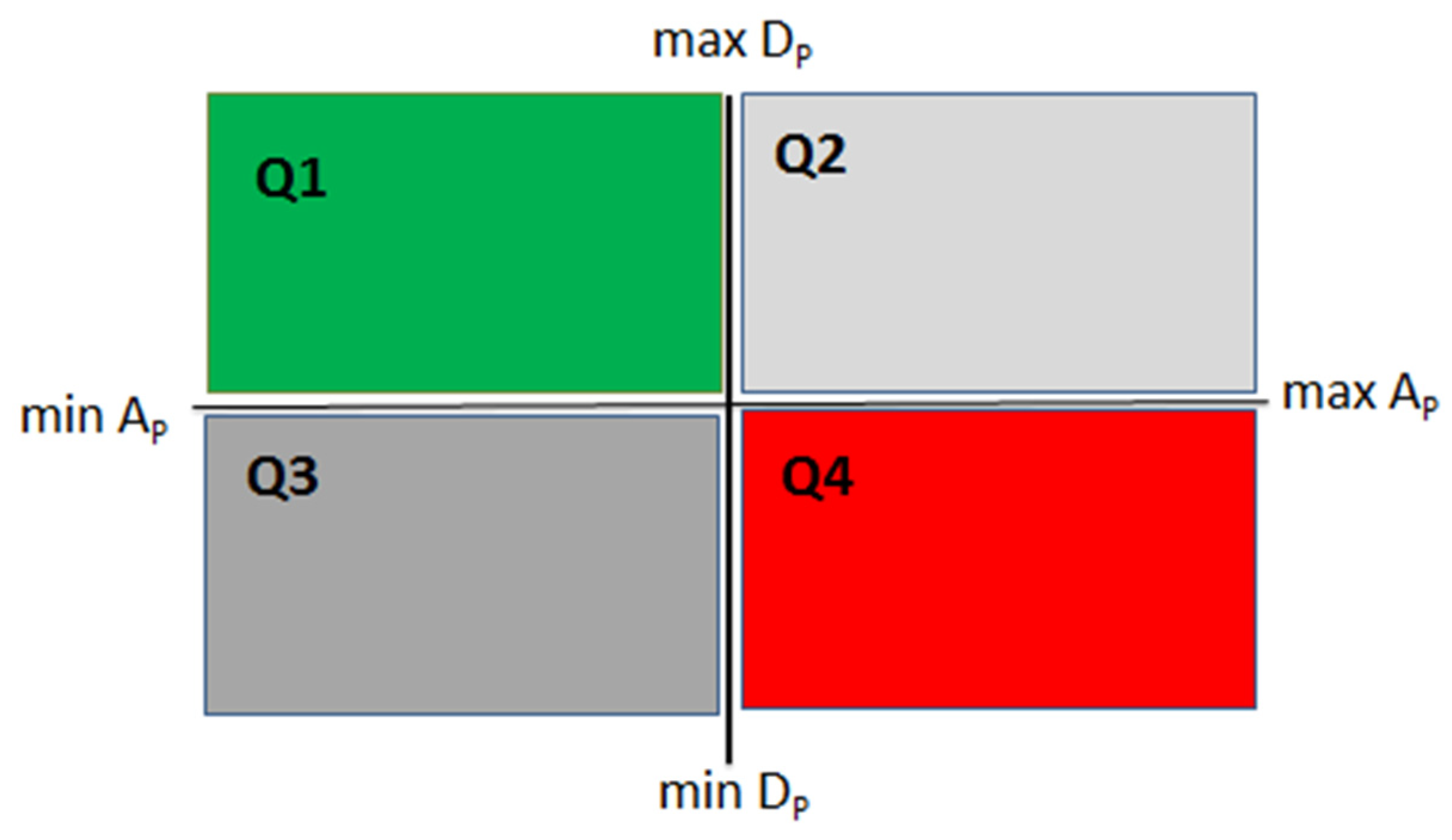
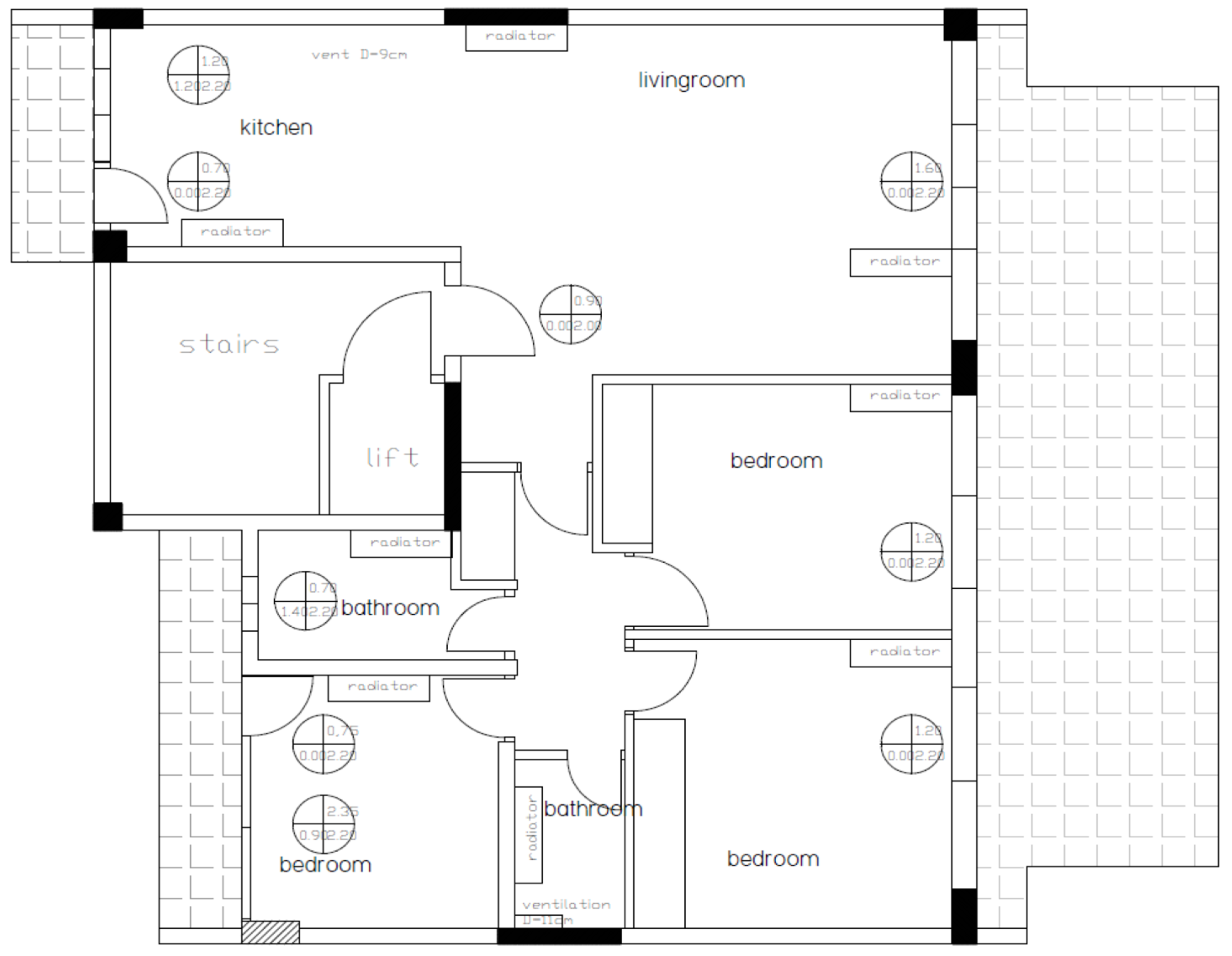
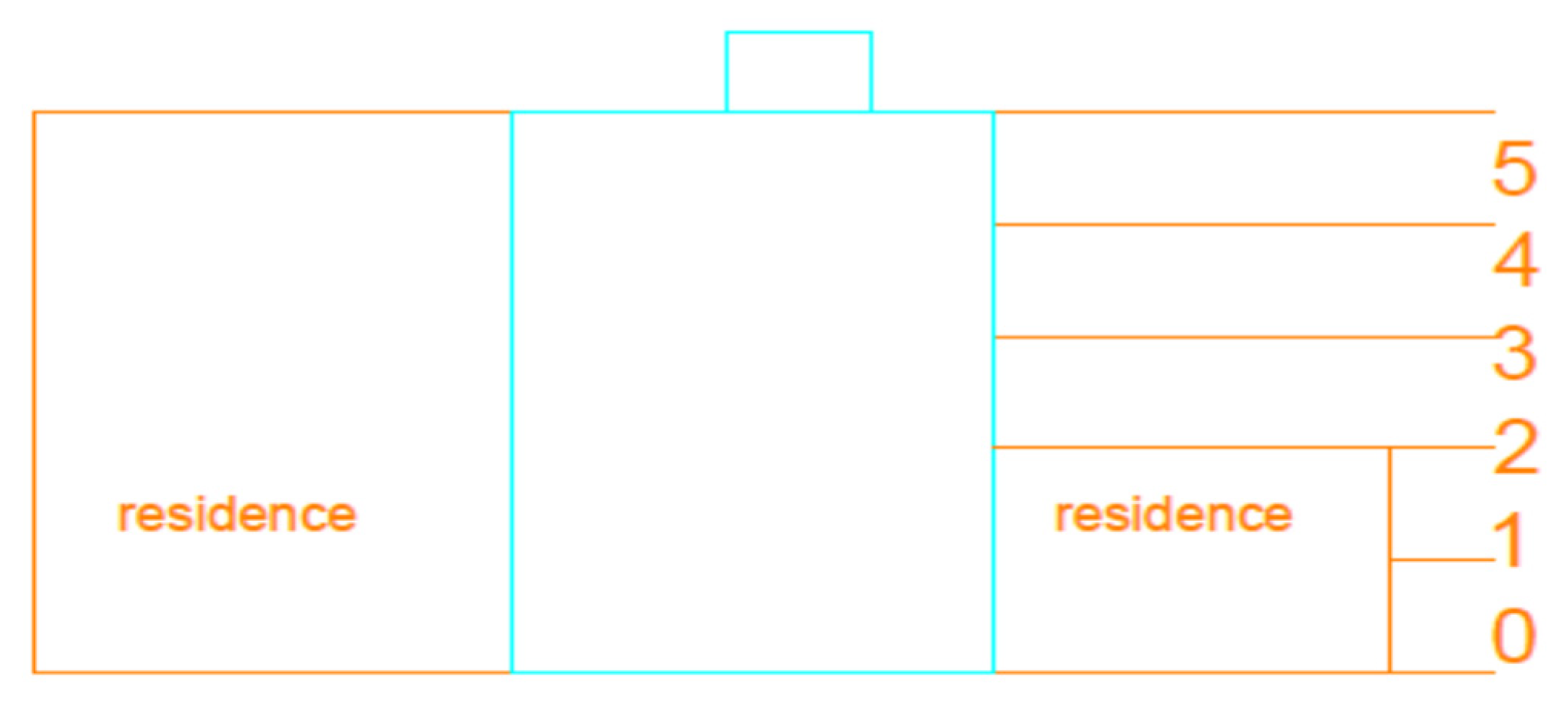
Table 1.
Basic area parameters of the apartment building shell.
| Flat Surface Area (m2) | |||||||
|---|---|---|---|---|---|---|---|
| Floor Level | Heated | Non-Heated | Total | Balcony | Cooled | % Non-Heated | Height (m) |
| Underground | 29.95 | 29.95 | 0 | 100 | 2.6 | ||
| Ground | 56.66 | 8.17 | 64.83 | 276 | 21.17 | 12.6 | 3.15 |
| Upper | 100.83 | 4.37 | 105.2 | 158.61 | 50.42 | 4.15 | 3.1 |
| Loft | 0 | 21.35 | 21.35 | 158.61 | 0 | 100 | 2.2 |
| Totals | 560.81 | 81.32 | 642.13 | 1227.66 | 273.24 | 17.02 | 23.45 |
| Flat Volume (m3) | |||||||
| Floor Level | Heated | Non-Heated | Total | Cooled | Perimeter (m) | Exterior Wall Area (m2) | |
| Underground | 0 | 77.87 | 77.87 | 0 | 22.34 | 58.08 | |
| Ground | 178.48 | 25.74 | 204.22 | 89.24 | 38.3 | 120.65 | |
| Upper | 312.57 | 13.55 | 326.12 | 156.29 | 50.44 | 156.36 | |
| Loft | 0 | 46.97 | 46.97 | 0 | 19 | 41.8 | |
| Totals | 1741.34 | 238.31 | 1959.65 | 870.67 | |||
Table 2.
Basic wall parameters of the building shell.
| Orientation (Degrees) | Total Area (m2) | Window Frames Area (m2) | Walls Area (m2) | U Wall (W/m2K) | |
|---|---|---|---|---|---|
| Wall no. 1 | 30 | 37.2 | 8.8 | 28.4 | 0.563 |
| Wall no. 2 | 120 | 27.75 | 27.75 | 0.522 | |
| Wall no. 3 | 210 | 26.35 | 8.12 | 18.24 | 0.521 |
| Wall no. 4 | 300 | 33.33 | 33.33 | 0.523 | |
| Stairway/elevator | 0 | 29.37 | 1.8 | 27.57 | 0.261 |
| Loft | 0 | 99.43 | 99.43 | 0.44 | |
| Maintenance room | 0 | 5.77 | 5.77 | 0.22 |
Table 3.
Nominal data for electromechanical systems and solar panel system data of the examined apartment unit.
Table 3.
Nominal data for electromechanical systems and solar panel system data of the examined apartment unit.
| Electromechanical Systems Nominal Data | ||||
|---|---|---|---|---|
| System | Source | Distribution | Season | Power(kW) |
| Heating | Oil | Yes | Winter | 80 |
| Cooling | Electricity | No | Summer | 7 |
| Hot water | Solar/Electricity | No | Year-round | 4 |
| Solar Panel System Data | ||||
| Panel tilt angle (degrees) | Panel area | Shade coefficient | Orientation(degrees) | |
| 37.58 | 4 | 1 | 180 | |
Table 4.
Controlling factors and their settings for the system design screening of the examined apartment unit.
Table 4.
Controlling factors and their settings for the system design screening of the examined apartment unit.
| SETTINGS | |||||
|---|---|---|---|---|---|
| FACTORS | CODE | -Boiler | -Heat Pump | +Boiler | +Heat Pump |
| Automation for water heating | FC1 | no | yes | ||
| Category of automatic control | FC2 | A | D | ||
| Number of ceiling fan (summer) | F3 | 0 | 5 | ||
| Type of heating systems | FC4 | boiler | Air-cooled h.p. | ||
| Energy source for heating systems | FC5 | Oil | Electricity | ||
| Power of heating systems (only for degree of efficiency) | F6 | 47.2 | 15.5 | 67.2 | 16.5 |
| Energy efficiency ratio of heating systems | F7 | 0.59 | 3.3 | 0.84 | 3.7 |
| Location of distribution network of heating systems | FC8 | Outdoor | Indoor | ||
| Efficiency of distribution network of heating systems | F9 | 0.86 | 0.96 | ||
| Efficiency of terminal units of heating systems | F10 | 0.83 | 1 | ||
| Type of cooling systems | FC11 | Air-cooled | water-cooled | ||
| Power of cooling systems (only for degree of efficiency) | F12 | 4 | 8 | ||
| Energy efficiency ratio of cooling systems | F13 | 1.5 | 3.72 | ||
| Efficiency of terminal units of cooling systems | F14 | 0.9 | 0.96 | ||
| Solar water heater | FC15 | Yes | No | ||
| Power of water heating systems (only for degree of efficiency) | F16 | 0.64 | 1.27 | ||
| Energy efficiency ratio of water heating systems | F17 | 0.85 | 1 | ||
| Recirculation of distribution network | FC18 | No | Yes | ||
| Efficiency of distribution network of water heating systems | F19 | 0.64 | 0.92 | ||
| Efficiency of the hot water storage container system | F20 | 0.93 | 0.98 | ||
| Type of auxiliary units for hot water | FC21 | No | 0.04 | circulator | |
| Type of solar panels | FC22 | Simple | Vacuum | - | |
| Utilization rate of solar water heating | F23 | 0.34 | 0.38 | - | |
| Surface area of solar panels | F24 | 2 | 5 | - |
Table 5.
The responses of the energy consumption (EC), intervention costs (IC), and their joint response (JR).
Table 5.
The responses of the energy consumption (EC), intervention costs (IC), and their joint response (JR).
| Run | EC (kWh/m2) | IC (EUR, €) | JR |
|---|---|---|---|
| 1 | 104.0 | 10,003 | 0.3633 |
| 2 | 163.4 | 9233 | 0.5897 |
| 3 | 149.2 | 7641 | 0.4402 |
| 4 | 105.7 | 16,815 | 0.7587 |
| 5 | 137.2 | 13,613 | 0.6364 |
| 6 | 132.7 | 20,302 | 0.9904 |
| 7 | 223.7 | 10,733 | 1.0791 |
| 8 | 204.1 | 3743 | 0.8363 |
| 9 | 197.7 | 13,028 | 0.9503 |
| 10 | 139.7 | 7894 | 0.3834 |
| 11 | 123.2 | 15,432 | 0.6970 |
| 12 | 146.3 | 20,975 | 1.0606 |
| 13 | 158.7 | 9892 | 0.5798 |
| 14 | 192.4 | 14,820 | 0.9791 |
Table 6.
The energy consumption (EC) response table.
| Factors | FC1 | FC2 | F3 | FC4 | FC5 | F6 | F7 | FC8 | F9 | F10 | FC11 | F12 |
|---|---|---|---|---|---|---|---|---|---|---|---|---|
| level - | 173.00 | 170.49 | 158.46 | 175.94 | 158.14 | 159.23 | 162.21 | 154.67 | 173.21 | 158.90 | 168.00 | 138.61 |
| level + | 138.14 | 140.66 | 152.69 | 135.20 | 153.00 | 151.91 | 148.93 | 156.47 | 137.93 | 152.24 | 143.14 | 172.53 |
| Difference | 34.86 | 29.83 | 5.77 | 40.74 | 5.14 | 7.31 | 13.29 | 1.80 | 35.29 | 6.66 | 24.86 | 33.91 |
| Rank | 3 | 5 | 18 | 1 | 19 | 16 | 11 | 23 | 2 | 17 | 6 | 4 |
| Factors | F13 | F14 | FC15 | F16 | F17 | FC18 | F19 | F20 | FC21 | FC22 | F23 | F24 |
| level - | 164.07 | 150.53 | 164.63 | 164.07 | 156.26 | 153.27 | 157.51 | 160.51 | 144.20 | 150.39 | 151.66 | 158.03 |
| level + | 147.07 | 160.61 | 146.51 | 147.07 | 154.89 | 157.87 | 153.63 | 150.63 | 166.94 | 160.76 | 159.49 | 153.11 |
| Difference | 17.00 | 10.09 | 18.11 | 17.00 | 1.37 | 4.60 | 3.89 | 9.89 | 22.74 | 10.37 | 7.83 | 4.91 |
| Rank | 9–10 | 13 | 8 | 9–10 | 24 | 21 | 22 | 14 | 7 | 12 | 15 | 20 |
Table 7.
Coefficients of regression analysis of EC (seven-factor strong group).
| Term | Coef | SE Coef | t-Value | p-Value | VIF |
|---|---|---|---|---|---|
| Constant | 192.0 | 11.9 | 16.20 | 0.000 | |
| FC1 | −36.27 | 8.84 | −4.10 | 0.006 | 1.57 |
| FC2 | −1.29 | 9.75 | −0.13 | 0.899 | 1.91 |
| FC4 | −31.57 | 8.33 | −3.79 | 0.009 | 1.39 |
| F9 | −13.91 | 9.30 | −1.50 | 0.185 | 1.74 |
| FC11 | −24.55 | 8.40 | −2.92 | 0.027 | 1.42 |
| F12 | 23.31 | 8.81 | 2.65 | 0.038 | 1.56 |
| FC21 | 11.37 | 8.55 | 1.33 | 0.232 | 1.47 |
Table 8.
Coefficients of the regression analysis of EC (four-factor confirmation).
| Term | Coef | SE Coef | t-Value | p-Value | VIF |
|---|---|---|---|---|---|
| Constant | 193.16 | 8.70 | 22.20 | 0.000 | |
| FC1 | −38.52 | 7.39 | −5.21 | 0.001 | 1.06 |
| FC4 | −35.42 | 7.44 | −4.76 | 0.001 | 1.07 |
| FC11 | −31.15 | 7.39 | −4.21 | 0.002 | 1.06 |
| F12 | 29.91 | 7.44 | 4.02 | 0.003 | 1.07 |
| Model Summary | |||||
| R2 | R2 (adj) | R2 (pred) | |||
| 90.80% | 86.71% | 75.88% | |||
| Regression Equation: | |||||
| EC = 193.16 − 38.52 FC1 − 35.42 FC4 − 31.15 FC11 + 29.91 F12 | |||||
Table 9.
Coefficients of regression analysis of the joint JR response (eight-factor strong group).
| Term | Coef | SE Coef | t-Value | p-Value | VIF |
|---|---|---|---|---|---|
| Constant | 1.0083 | 0.0926 | 10.89 | 0.000 | |
| FC1 | −0.1810 | 0.0470 | −3.85 | 0.012 | 1.42 |
| FC2 | −0.1653 | 0.0525 | −3.15 | 0.025 | 1.77 |
| FC4 | −0.1619 | 0.0502 | −3.23 | 0.023 | 1.62 |
| F6 | −0.0499 | 0.0479 | −1.04 | 0.345 | 1.47 |
| FC8 | −0.2581 | 0.0632 | −4.09 | 0.009 | 2.56 |
| FC11 | −0.0501 | 0.0543 | −0.92 | 0.399 | 1.89 |
| FC12 | −0.0306 | 0.0528 | −0.58 | 0.587 | 1.79 |
| F19 | 0.2496 | 0.0486 | 5.14 | 0.004 | 1.51 |
Table 10.
Coefficients of regression analysis of joint JR response (five-factor confirmation).
| Term | Coef | SE Coef | T-Value | p-Value | VIF |
|---|---|---|---|---|---|
| Constant | 0.9953 | 0.0443 | 22.48 | 0.000 | |
| FC1 | −0.1882 | 0.0456 | −4.13 | 0.003 | 1.36 |
| FC2 | −0.1687 | 0.0504 | −3.35 | 0.010 | 1.66 |
| FC4 | −0.1627 | 0.0449 | −3.62 | 0.007 | 1.32 |
| F19 | 0.2339 | 0.0409 | 5.72 | 0.000 | 1.10 |
| FC8 | −0.2271 | 0.0421 | −5.40 | 0.001 | 1.16 |
| Model Summary | |||||
| R2 | R2 (adj) | R2 (pred) | |||
| 94.73% | 91.43% | 85.96% | |||
| Regression Equation | |||||
| JR = 0.9953 − 0.1882 FC1 − 0.1687 FC2 − 0.1627 FC4 − 0.2271 FC8 + 0.2339 F19 | |||||
Table 11.
The corrected Akaike information criterion scores for sequential factor screening of the EC response.
Table 11.
The corrected Akaike information criterion scores for sequential factor screening of the EC response.
| Factor Group | Sum of | p | n | AICc |
|---|---|---|---|---|
| Squares | ||||
| FC4 | 11,822.58 | 3 | 14 | 102.74 |
| FC4, FC1 | 8810.14 | 4 | 14 | 102.67 |
| FC4, FC1, FC11 | 4538.14 | 5 | 14 | 98.44 |
| FC4, FC1, FC11, F12 | 1622.77 | 6 | 14 | 90.54 |
| FC4, FC1, FC11, F12, F9 | 1365.94 | 7 | 14 | 96.79 |
| FC4, FC1, FC11, F12, F9, FC18 | 647.7 | 8 | 14 | 98.48 |
Table 12.
The corrected Akaike information criterion scores for sequential factors screening the JR response.
Table 12.
The corrected Akaike information criterion scores for sequential factors screening the JR response.
| Important Factor Group | Sum of | p | n | AICc |
|---|---|---|---|---|
| Squares | ||||
| FC2 | 0.3925 | 3 | 14 | −41.64 |
| FC2, FC1 | 0.3114 | 4 | 14 | −40.84 |
| FC2, FC1, FC8 | 0.2293 | 5 | 14 | −40.06 |
| FC2, FC1, FC8, F19 | 0.097 | 6 | 14 | −45.61 |
| FC2, FC1, FC8, F19, FC4 | 0.0367 | 7 | 14 | −50.55 |
| FC2, FC1, FC8, F19, FC4, FC15 | 0.0255 | 8 | 14 | −43.51 |
| FC2, FC1, FC8, F19, FC15 | 0.0441 | 7 | 14 | −47.98 |
Table 13.
A comparative energy performance evaluation of the original energy status of the examined apartment unit against a recommended renovation.
Table 13.
A comparative energy performance evaluation of the original energy status of the examined apartment unit against a recommended renovation.
| Settings | |||
|---|---|---|---|
| FACTORS | CODE | Original Status | EC Solution |
| Automation for Hot Water | FC1 | no | Yes |
| Category of automatic control (choice among 4) | FC2 | C | D |
| Number of ceiling fan (summer) | F3 | 0.00 | 5.0 |
| Type of heating systems (select from a list) | FC4 | boiler | Air-cooled heating pump |
| Energy source for heating systems (select from a list) | FC5 | Oil | Oil |
| Power of heating systems (only for degree of efficiency) | F6 | 47.20 | 67.20 |
| Energy efficiency ratio of heating systems | F7 | 0.59 | 0.84 |
| Location of distribution network of heating systems | FC8 | Indoor | Indoor |
| Efficiency of distribution network of heating systems | F9 | 0.86 | 0.96 |
| Efficiency of terminal units of heating systems | F10 | 0.84 | 1 |
| Type of cooling systems (select from a list) | FC11 | Air-cooled | Water-cooled |
| Power of cooling systems (only for degree of efficiency) | F12 | 4.76 | 4.0 |
| Energy efficiency ratio of cooling systems | F13 | 2.36 | 3.72 |
| Efficiency of terminal units of cooling systems | F14 | 0.96 | 0.90 |
| Solar water heater | FC15 | Yes | No |
| Power of heating water systems (only for degree of efficiency) | F16 | 1.27 | 1.27 |
| Energy efficiency ratio of heating water systems | F17 | 1 | 1 |
| Recirculation of distribution network (yes or no) | FC18 | No | No |
| Efficiency of distribution network of heating water systems | F19 | 0.84 | 0.92 |
| Efficiency of domestic hot water storage system | F20 | 0.93 | 0.98 |
| Type of auxiliary units (select from a list) for domestic hot water | FC21 | No | No |
| Type of solar panels (choice among 3) | FC22 | Simple | Simple |
| Utilization rate of solar radiation for domestic hot water | F23 | 0.34 | 0.34 |
| Surface area of solar panels | F24 | 4.00 | 5.00 |
| Energy Consumption of the apartment unit (kWh/m2): | 156.3 | 83.3 | |
| Energy Consumption of the reference apartment unit (kWh/m2): | 123.5 | 75.1 | |
| Energy Status Grade (Certification level): | C | B |
Publisher’s Note: MDPI stays neutral with regard to jurisdictional claims in published maps and institutional affiliations. |
© 2022 by the authors. Licensee MDPI, Basel, Switzerland. This article is an open access article distributed under the terms and conditions of the Creative Commons Attribution (CC BY) license (https://creativecommons.org/licenses/by/4.0/).
Share and Cite
MDPI and ACS Style
Rousali, C.; Besseris, G. Lean Screening for Greener Energy Consumption in Retrofitting a Residential Apartment Unit. Appl. Sci. 2022, 12, 6631. https://0-doi-org.brum.beds.ac.uk/10.3390/app12136631
AMA Style
Rousali C, Besseris G. Lean Screening for Greener Energy Consumption in Retrofitting a Residential Apartment Unit. Applied Sciences. 2022; 12(13):6631. https://0-doi-org.brum.beds.ac.uk/10.3390/app12136631
Chicago/Turabian StyleRousali, Christina, and George Besseris. 2022. "Lean Screening for Greener Energy Consumption in Retrofitting a Residential Apartment Unit" Applied Sciences 12, no. 13: 6631. https://0-doi-org.brum.beds.ac.uk/10.3390/app12136631
Note that from the first issue of 2016, this journal uses article numbers instead of page numbers. See further details here.