
Automated Geological Features Detection in 3D Seismic Data Using Semi-Supervised Learning


Department of Geosciences, Universiti Teknologi PETRONAS, Seri Iskandar 32610, Malaysia
*
Authors to whom correspondence should be addressed.
Appl. Sci. 2022, 12(13), 6723; https://0-doi-org.brum.beds.ac.uk/10.3390/app12136723
Submission received: 15 June 2022
/
Revised: 28 June 2022
/
Accepted: 28 June 2022
/
Published: 2 July 2022
(This article belongs to the Special Issue Artificial Intelligence Applications in Petroleum Exploration and Production)
Abstract
:Featured Application
This article demonstrates the use of a type of semi-supervised learning to automatically de-tected geological features in seismic data.
Abstract
A geological interpretation plays an important role to gain information about the structural and stratigraphic of hydrocarbon reservoirs. However, this is a time-consuming task due to the complexity and size of seismic data. We propose a semi-supervised learning technique to automatically and accurately delineate the geological features from 3D seismic data. To generate labeling data for training the supervised Convolutional Neural Network (CNN) model, we propose an efficient workflow based on unsupervised learning. This workflow utilized seismic attributes and KernelPCA to enhance the visualization of geological targets and clustering the features into binary classes using K-means approach. With this workflow, we are able to develop a data-driven model and reduce human subjectivity. We applied this technique in two cases with different geological settings. The synthetic data and the real seismic investigation from the A Field in the Malay Basin. From this application, we demonstrate that our CNN-based model is highly accurate and consistent with the previous manual interpretation in both cases. In addition to qualitatively evaluating the interpretations, we further extract the predicted result into a 3D geobody. This result could help the interpreter focus on tasks requiring human expertise and aid the model’s prediction in the next studies.
1. Introduction
The first step of successful hydrocarbon discovery is to understand the structure of exploration targets in the subsurface. It is, therefore, important to understand all subsurface components, including the sedimentological and geological features. These geological features consist of faults, folds, anticlines, salt, channels, etc. [1]. Seismic reflection imaging is the common method to differentiate each geological features in subsurface [2]. The interpretation of seismic imaging data from 3D horizon/time slices enables the recognition and characterization of detailed geological features. Seismic interpretation is often dependent on the interpreter’s experience and knowledge. Hence, this task is both a subjective process and a time-consuming task, especially in the case of large and complex seismic data.
To address this issue, research using artificial intelligence with the help of advanced computing technology has drawn a lot of attention in recent years to automatically interpret the geological features in seismic data. This trend drives scientists to apply various types of artificial intelligence methods. Basically, artificial intelligence can be divided into two major categories, namely supervised and unsupervised learning techniques. The main difference between these two categories is the requirement for data labeling. The supervised learning technique is a method that involves data labeling, i.e., classification and regression problems, while the unsupervised learning technique is a method without involving data labeling, i.e., clustering and dimensionality reduction [3].
A particular supervised learning method has shown tremendous success in detect geological features on seismic data, including the detection of salt bodies [4,5,6], the delineation of faults [7,8], and classification different type of seismic facies [9,10,11,12]. Several studies also used the unsupervised learning method to detect the geological features, for example, by using principal component analysis [13], K-means clustering [14,15], a self-organizing map (SOM) [16], and a convolutional autoencoder [17].
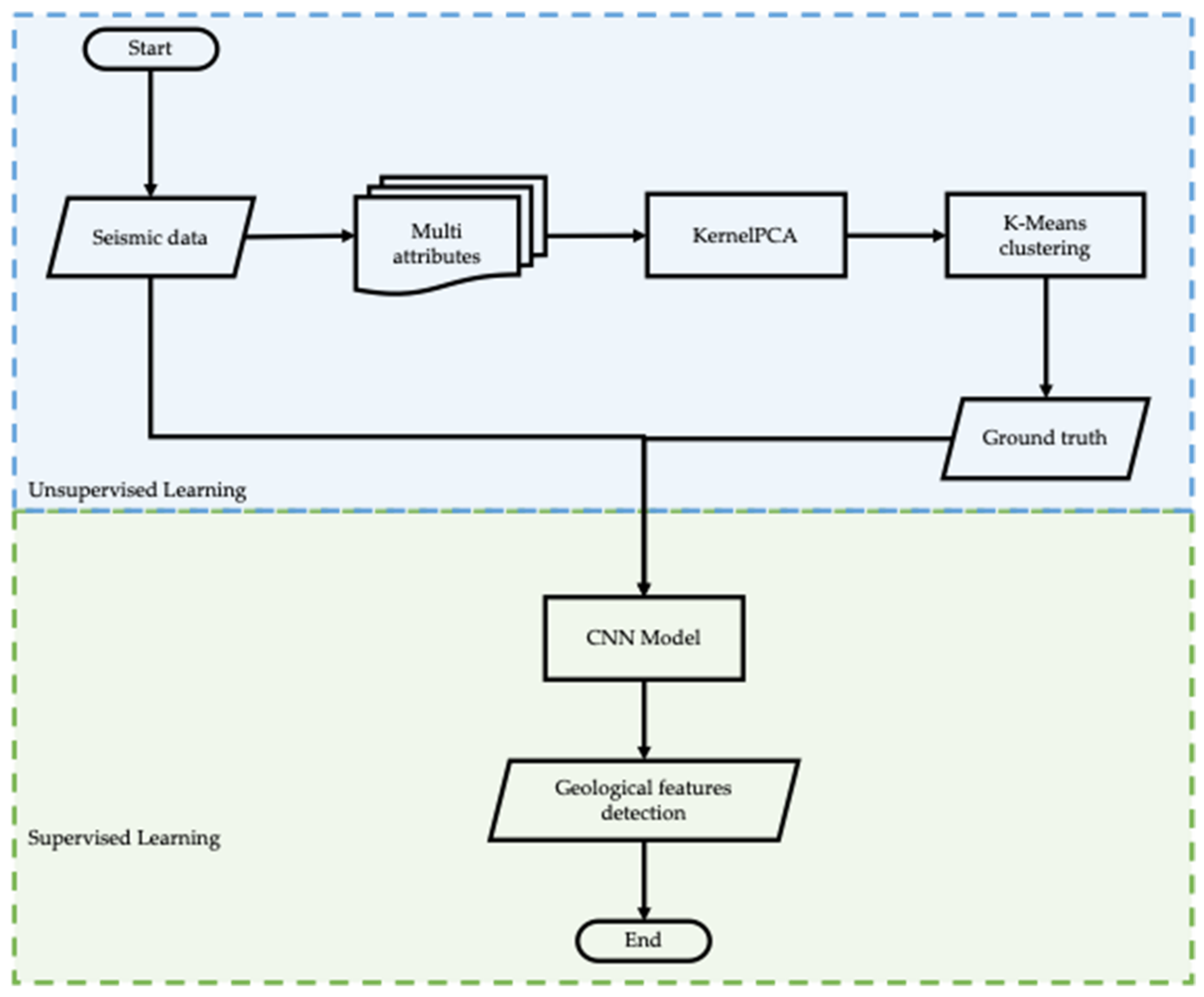
In this paper, we consider combining supervised and unsupervised learning techniques into semi-supervised learning methods. By using an unsupervised learning approach, we will design an enhanced workflow to generate the label data that will be used to develop the supervised model. This workflow starts by applying several seismic attributes to the seismic data to help visually enhance or quantify geological features of interest. Then, we used the dimensionality reduction technique to reduce and combine multi-attribute analysis into some various principal components. Finally, using these principal components, we applied a clustering technique to generate the labeling data. This proposed workflow can help us generate a fair amount of data for the model building process, where manual labeling is challenging. Additionally, the unsupervised learning approach is a more data-driven way to determine the geological labels present in the seismic data, without being affected by interpreters’ biases.
For the model building, we applied a supervised learning approach by using one of the deep learning techniques called Convolutional Neural Network (CNN). Consider the geological features detection in seismic data as an image segmentation problem. We solve this problem using a modified CNN’s architecture called U-Net [18]. In order to get the accurate prediction, we fine-tuned the model hyperparameters, including network architecture, loss technique, activation function, and many more [19]. We also applied the transfer learning technique by reusing the comprehensively pre-trained model in other datasets to our architecture’s backbone [20].
This paper proposes an enhanced workflow based on a semi-supervised learning approach to detect geological features in 3D seismic data automatically. The structure of this paper is organized as follows. First, we start by discussing two 3D seismic data, including synthetic and real seismic surveys, with the related geological background. The synthetic seismic is from the SEAM seismic dataset, while the real seismic is from the A Field in the Malay Basin. We then present the proposed workflow to generate data labels for model development. We further discussed the architecture of the CNN model and trained it with different hyperparameter selections. Finally, we applied this workflow with two 3D seismic datasets and compared the result with manual interpretation from a previous study as the evaluation process.
2. Seismic Data and Geological Background
2.1. SEAM Synthetic Seismic Dataset
The SEAM Phase I synthetic seismic dataset was designed to represent a deepwater Gulf of Mexico salt domain field. This dataset was modeled with complex and realistic geological features, including faults, overturned beds, overhanging salt, turbidite fans, and braided stream channels reservoir [21].
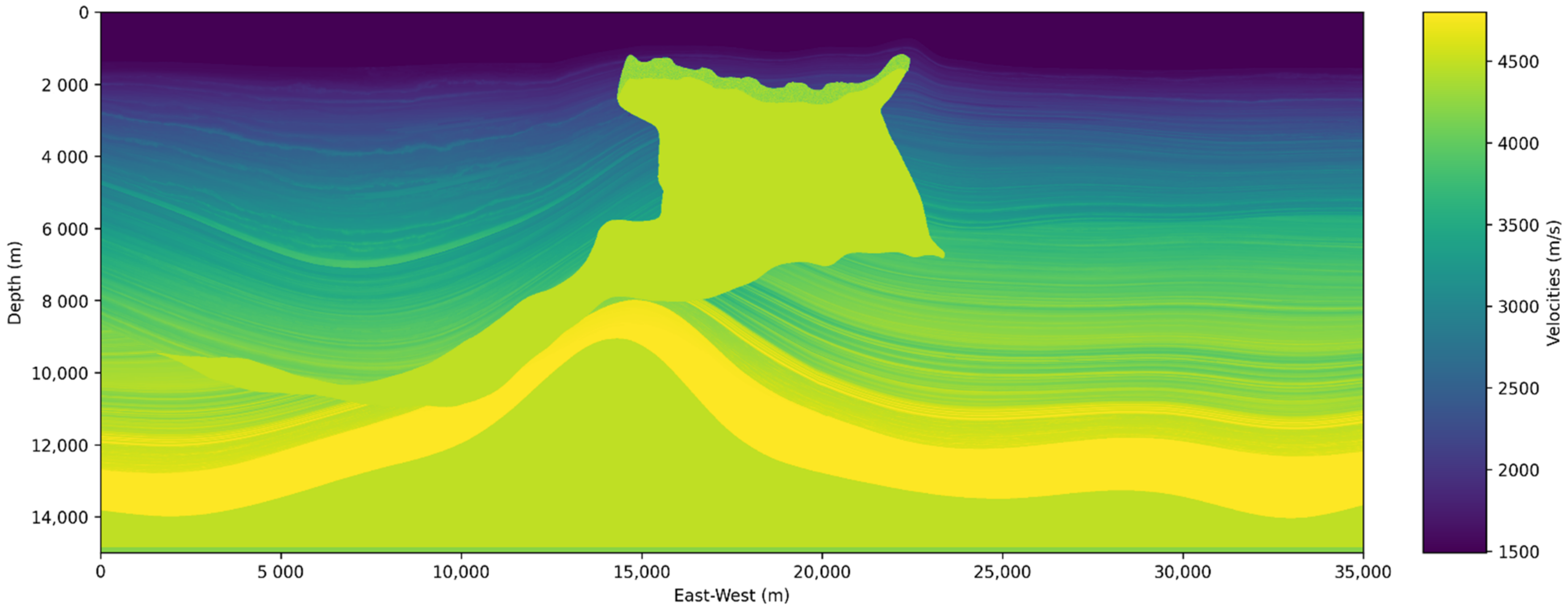
The main advantage of using synthetic seismic data is that the location of geological features is known in the seismic section. Thus, it will be convenient to evaluate the proposed workflow and model on this synthetic dataset. The salt body is the main geological feature in the SEAM dataset. This salt body is reflected in the behavior of velocity values. The velocity in salt body is generated as a uniform random distribution of values centered at 4280 m/s [21]. Figure 1 shows the velocity values on SEAM seismic section.
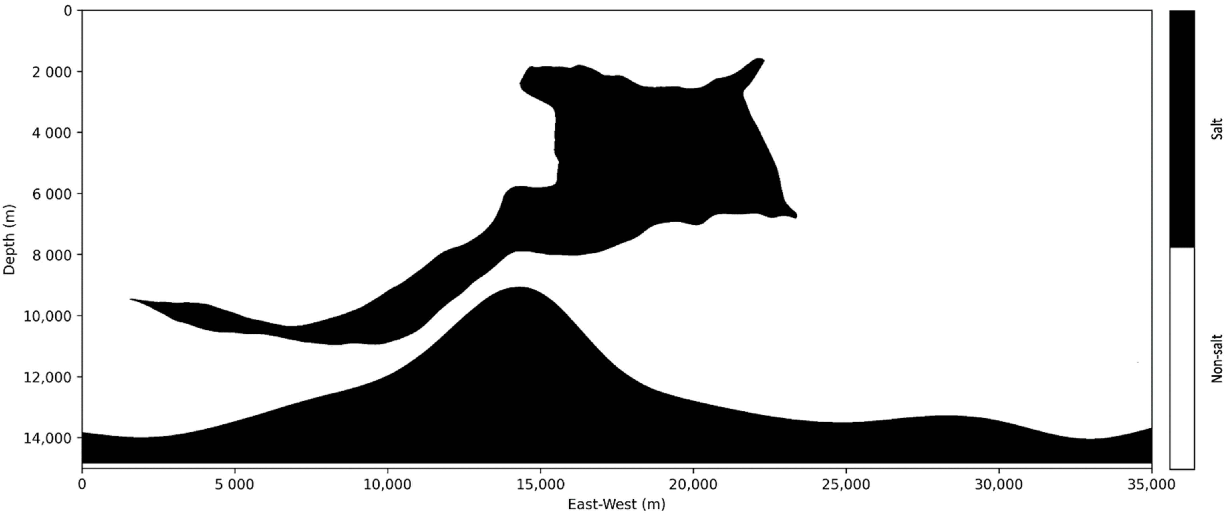
According to the velocity values, this salt body is made up of two parts: the overhanging salt and the mother salt. According to Figure 2, the convex surface at the bottom of the figure represents the mother salt, while the overhanging salt is shown in the middle of the figure.
2.2. The A Field Real Seismic Dataset
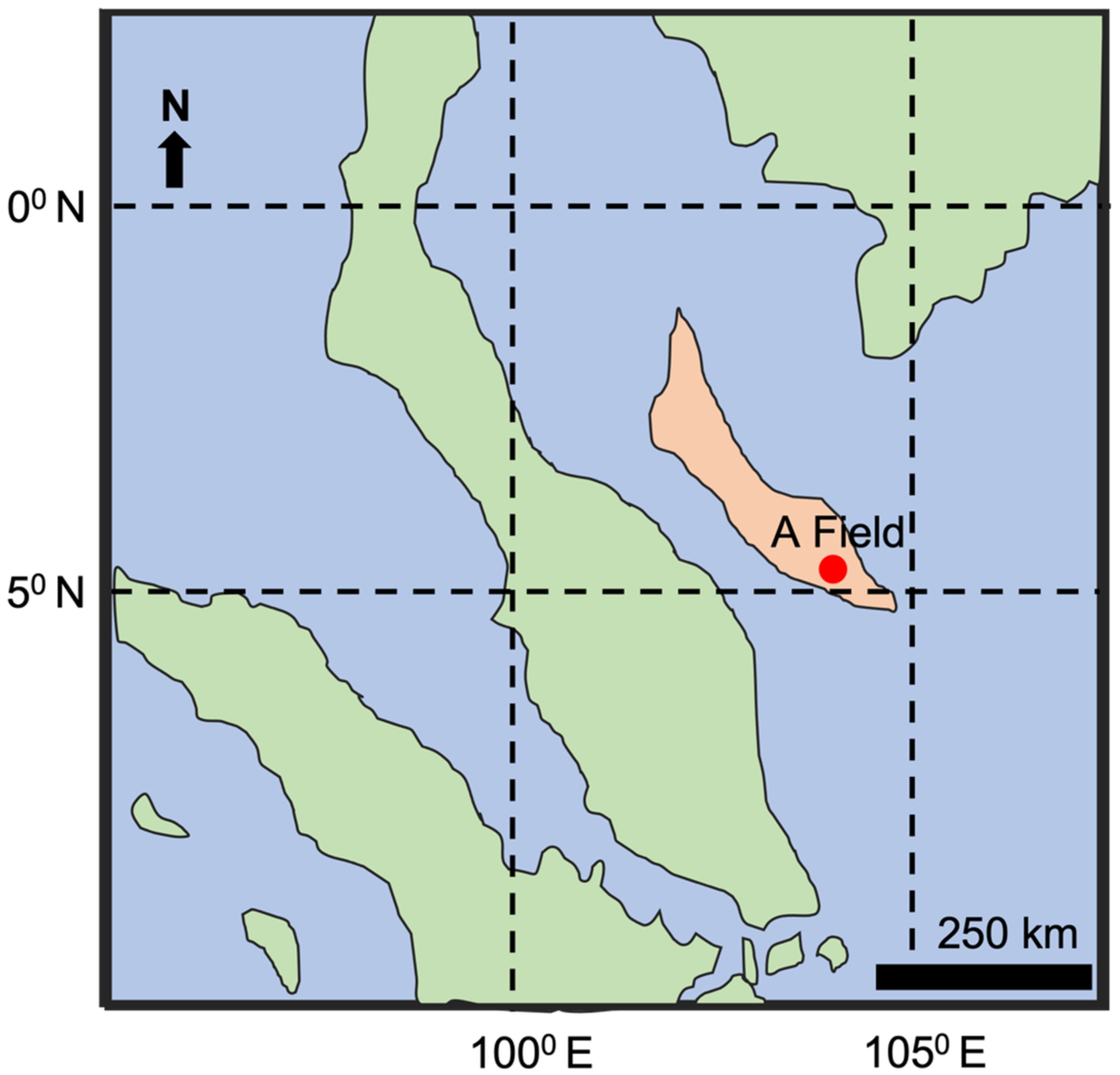
In this paper, the A Field in the Malay basin is used to test the proposed workflow and model on real seismic data. The A Field is located in the offshore of Peninsular Malaysia, which lies in the southern part of the Malay Basin (Figure 3) [22].
The field is covered by the seismic survey at the center of Malay Basin, running in the NW to SE direction elongated with anticline structural dips ranging from 1 to 3 degrees. There are E-W trending normal faults that delineate at the main reservoir; additionally, the youngest N-S faults present at the flank of the field occur throughout the reservoirs [23].
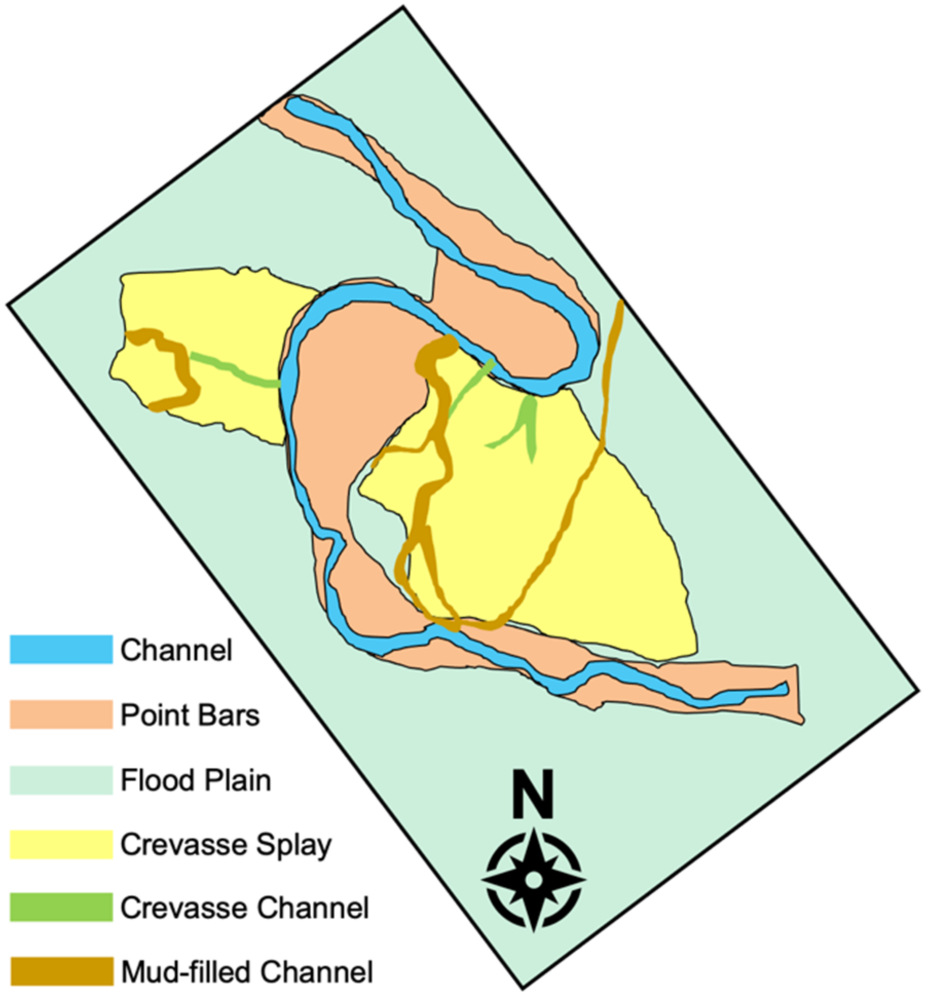
The A Field was interpreted as the meandering fluvial channel environment reservoir [24]. A significant amount of commercial hydrocarbon can be found on the channel sand-body reservoir. Hence, it is crucial to interpret and predict the structure and geometry of the channel features. All the identified channel features in this seismic field are classified based on fourth-order meandering fluvial hierarchical architecture, which consisted of a point bar, an abandoned channel, crevasse splays, and a flood plain [25]. By integrating the seismic result to the well log information, the previous study interpreted six channel features in the data, which consist of a flood plain, channel, point bar, crevasse splay, crevasse channel, and mud-filled channel, as shown in Figure 4 [24].
3. Enhanced Labeling Workflow
To build a CNN model for detecting the geological features in 3D seismic data, we propose an enhanced workflow (as shown in Figure 5) to automatically generate many labeled geological features related with the seismic data. We applied several seismic attributes and unsupervised learning techniques, including dimensionality reduction and clustering that can automatically and perfectly label the obtained target seismic data for training the CNN.
3.1. Seismic Attributes Selection
In this workflow, we begin by selecting and applying several seismic attributes to the seismic data. A seismic attribute is a measure of a seismic property that helps visually enhance and quantify the geological features of interest [26]. Seismic wave can be represented by three important variables, namely amplitude, phase, and frequency [27]. Each of these variables represents different attributes that help bring out different aspects of the geological feature.
The amplitude variable can be used to strengthen the reflection. This technique is suitable to find the potential hydrocarbon accumulation or sweet spot in the seismic data, which indicates the better net to gross reservoir sands. On the other hand, frequency variable signifies the resolution that can be used to detect thin beds and different depositional environments. The phase variable is primarily an indicator of structural discontinuities, such as faults, salts, and other geomorphological features [28].
Seismic attribute selection begins by choosing suitable attributes for the geological feature target. Table 1 summarizes the most commonly used attributes that measure seismic properties and their specific geological applications.
In this paper, we focus on the attribute selection for salt and channel features as per the environment of deposition on each seismic dataset. The structural seismic attributes are important to quantify and detect the salt structure. These attributes are discontinuity, dip, azimuth, curvature, and amplitude change. The salt structure identified by the high velocity and strong acoustic impedance contrasts with surrounding sediments [29]. Salt interpretation consists of two complementary steps: first, highlighting the salt boundaries in the seismic data; second, extracting the boundaries by creating three dimensional surfaces [30].
For the channel features, seismic geomorphology attributes (i.e., curvature, dip, azimuth, etc.) can provide the channel’s internal and external sinuosity architecture [31]. Seismic attributes based on the amplitude value are also show tremendous result on highlighting reservoir channel features that contain point-bar accretion and stacking pattern [32]. Lateral variations in reservoir quality and thickness follow scrollbar patterns associated with lateral migration of a moderate-to-high-sinuosity meandering river [33].
3.2. Dimensionality Reduction Algorithm
In order to get the best visualization of the detected geological features by each attribute, the multi-attributes analyses can be combined and reduced into some meaningful principal components. This idea is known as Principal Components Analysis (PCA) and is classified as an unsupervised learning method. However, this technique is based on linear transformation, whereas seismic multi-attributes analysis is a non-linear problem; thus, it will not fit well in the seismic multi-attributes analysis [34].
To address this problem, there is a kernel based PCA technique that is fit for processing non-linear problems, and can reduce the dimension of the data without much loss of information [35]. The methods behind the KernelPCA algorithm are the same as PCA, which tends to maximize the variance of the transformed result in feature space. The main difference is the kernel technique that have been used in KernelPCA. This kernel is used to implement PCA in hyperspace, which can induce the originally scattered samples to aggregate along the eigenvector direction. The main idea of the kernel method was applied to the Support Vector Machine (SVM) algorithm firstly [36].
3.3. Clustering Algorithm
The next step of this proposed workflow consists of applying the clustering algorithm to the principal components output in order to get the cluster that represents the geological features. We choose K-means clustering as the clustering algorithm. K-means clustering is an unsupervised method designed to split unlabeled data distribution into a fixed number K of clusters which share common characteristics for each group [37].
Basically, the K-means algorithm’s objective is to reduce the error between each data point and K centroid, using the following equation:
where the is the distance indicator of the n dataset points and is the representation of K centroids. Usually, the distance is measured with the Euclidean distance [38]. The K-means algorithm composed with the following four steps [39]:
- Place K centroid in randomly in space, which represent the item coordinates that are being clustered;
- Group each item in the group that have the same similarity to it;
- Recompute the K centroid and change their position, respectively;
- Iterate step (2) and (3) until the position of the K centroid does not change with respect to the distances between all the elements of their group.
After receiving the optimum result of K-means clustering, we assigned those clustered result as the label for our geological features that we wanted to detect. This result will be the ground truth or the true output that will be used on the training model.
3.4. Training Dataset
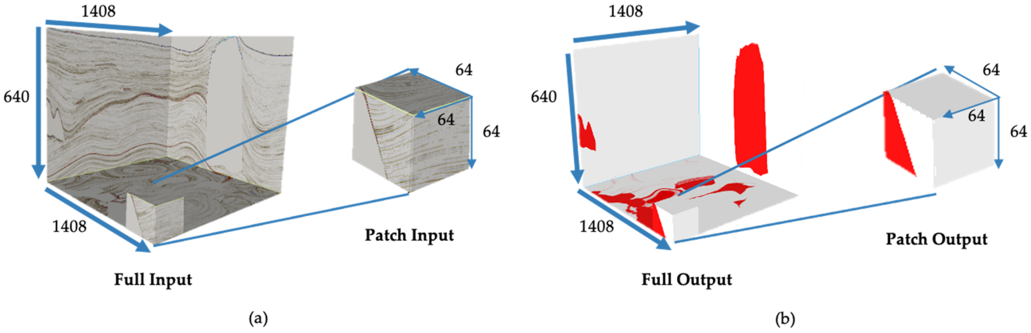
In this presented study, we trained and applied the model on the 3D seismic volume, which has a large amount of data. Thus, we need to divide those large seismic volumes before feeding them into the model to address the computing limitation. We divided the whole seismic volume into small cubes, namely the seismic patches. We designed those patches with a size of 64 × 64 × 64 and then performed the scaling process, so that it would fit well into the CNN architecture. The same conditions also applied to the ground truth volume, which we divided into small patches to feed into the network as the output (Figure 6).
We generate 384 pairs of seismic patches and their correlated ground truth as the input and output for the training process. We selected these pair patches in random locations in the original seismic data. In total, 80% of the dataset will be used for training and the rest for validation.
4. Deep Learning for Detecting Geological Features
The geological features detection can be classified as the image segmentation problem in the computer vision field. The image segmentation problem will classify each pixel of the image into one of the predefined classes [40]. Considering the seismic section as an image, we divided the section into small patches to feed into the deep learning model and assign the seismic interpretation problems as the image classification problem [17].
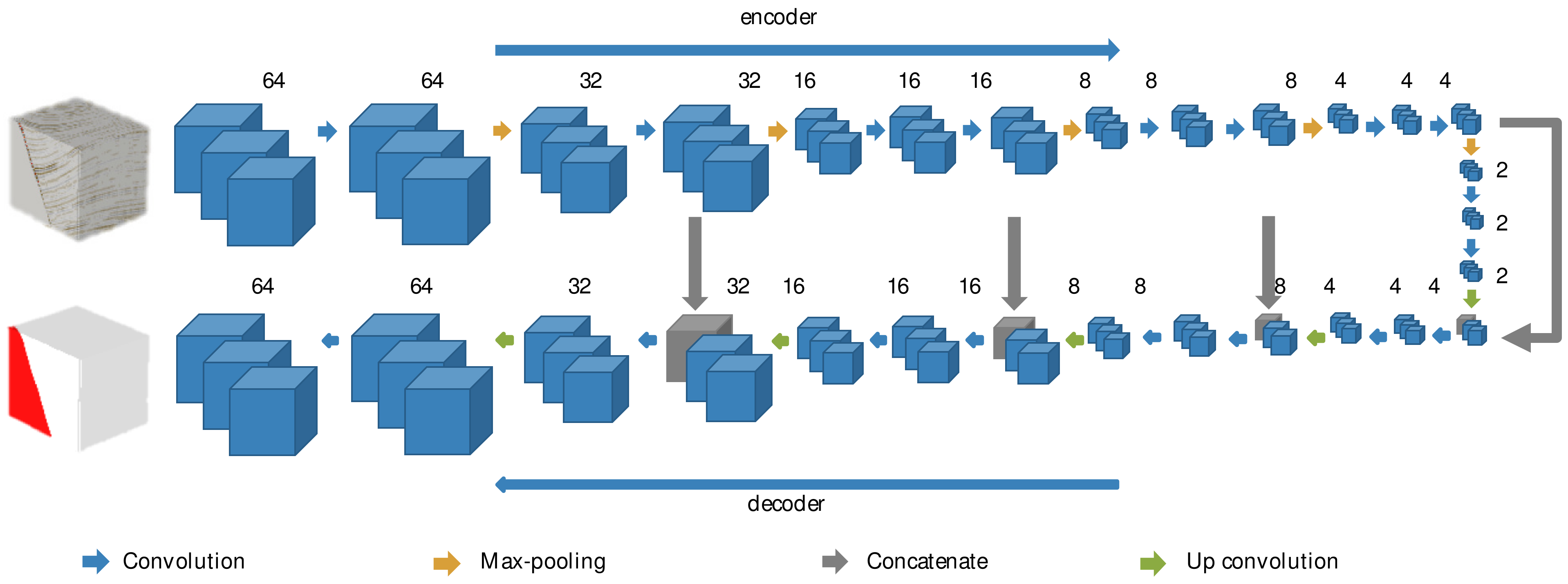
Convolutional Neural Network (CNN) is a very useful tool for image classification and segmentation. CNN is a specialization of neural networks for data in the form of multiple arrays, such as images or seismic data [41]. A particular of CNN architectures, U-Net, has shown tremendous success in image segmentation problems. This U-shaped network was originally proposed by Ronneberger in 2015 for medical image segmentation [18]. We adopted and modified this architecture to fit our problem as shown in Figure 7. Similar to the original U-Net, the modified architecture still has the encoder (top) and decoder (bottom) parts.
In the encoder part, we feed the network with a small patch of seismic data of 64 × 64 × 64 size. The input will be convolved with 3 × 3 × 3 filters to obtain the feature maps. Each step consists of two 3 × 3 × 3 convolutional layers followed by a Sigmoid activation function, as formulated with:
where is the prediction result from each layer in the network. The main advantage of using Sigmoid as the activation function is that the output is a probability between 0 and 1, which signifies how confident the model predicted the class [42].
The 2 × 2 × 2 max-pooling is also applied in each step, so the size of the layers will be reduced from 64 at the first step to 32, 16, 8, 4, and 2 at the final of the encoder part. The bottleneck structure at the middle of the encoder and decoder part consists of 3 × 3 × 3 convolutional layers. Then, the upconvolutional process is implemented at the decoder part to resize the layer into the original one followed by a concatenation process from the encoder part to gain the localization information.
The network will keep updating the weights for each layer using the optimization algorithm until the minimum error between the predicted result and labeled output has been achieved. We use the binary cross-entropy to measure the error with the following formula:
where the is the target and is the prediction at -th. We iteratively optimize the parameters during the training process with 1000 epochs using the Adam optimizer [43], with 0.0001 as the learning rate. In the encoder part, we also implemented the transfer learning methods. We use Resnet-50 as the base model, pre-trained for the object detection tasks on the ImageNet dataset [20,44]. Despite the disparity between the natural image on the ImageNet dataset and geological features on our seismic dataset, Resnet-50 comprehensively trained on the ImageNet can be transferred to make geological features detection more effective, since collecting and labeling large numbers of geological features on seismic data still poses significant challenges [12]. Table 2 shows the hyperparameter and the selected parameters used to build the CNN model.
To objectively evaluate the performance of our models on this dataset, we use a set of evaluation metrics that are commonly used in segmentation and classification problems.
In this paper, we are going to use confusion metrics and Intersection over Union (IoU) metrics as the evaluation metrics.
A confusion matrix, also known as an error matrix, is a specific table layout that allows visualization of the performance of an algorithm [45]. There are four basic terms in a confusion matrix:
- True Positives (TP): positive outcomes are predicted, and they are true;
- True Negatives (TN): negative outcomes are predicted, and they are true;
- False Positives (FP): positive outcomes are predicted, but they are false;
- False Negatives (FN): negative outcomes are predicted, but they are false.
From the information above, we can derive the following equations:
The IoU metric, also known as the Jaccard index, is the most commonly used metric for comparing the similarity between two arbitrary shapes [46]. IoU is formulated as:
5. Applications
To apply and verify this propose workflow and model, we apply the workflow and train the CNN model to both the synthetic and real 3D seismic dataset. As shown in Figure 5, we start with the unsupervised part to generate the ground truth data as the output, then, together with seismic data as the input, we develop the CNN model.
5.1. SEAM Synthetic Seismic Example
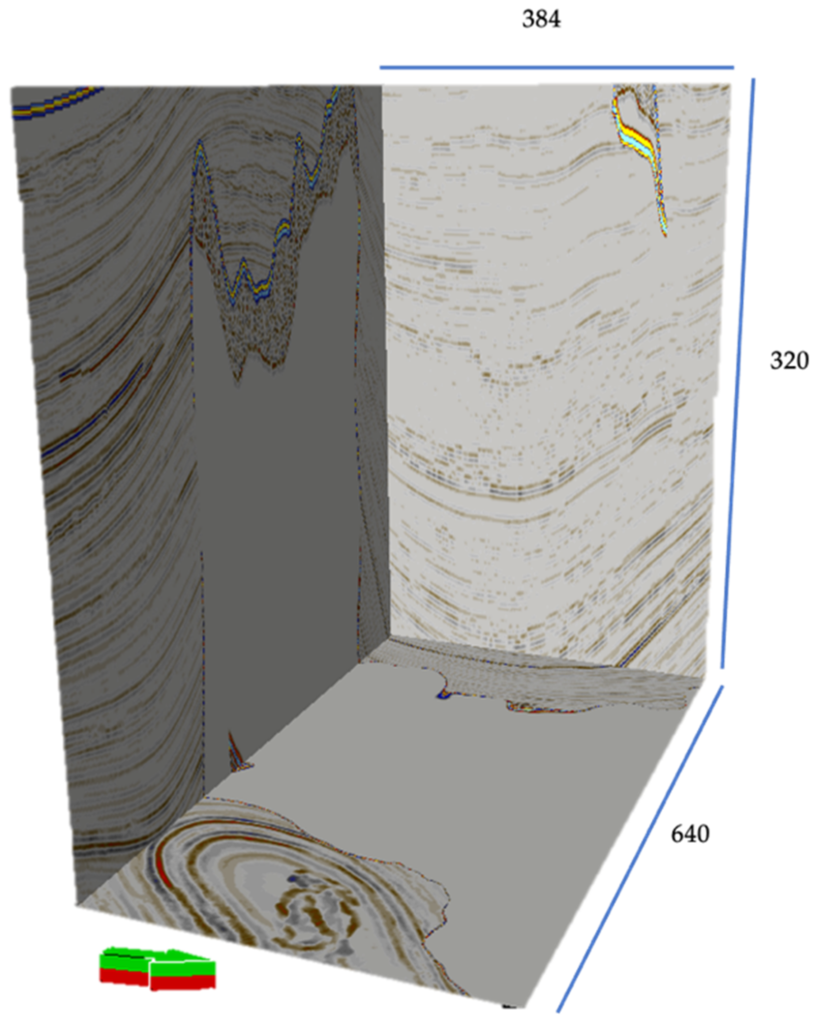
SEAM 3D seismic cube consists of 640 inline, 384 crossline, and 320 time-slice. Figure 8 shows the whole seismic volume.
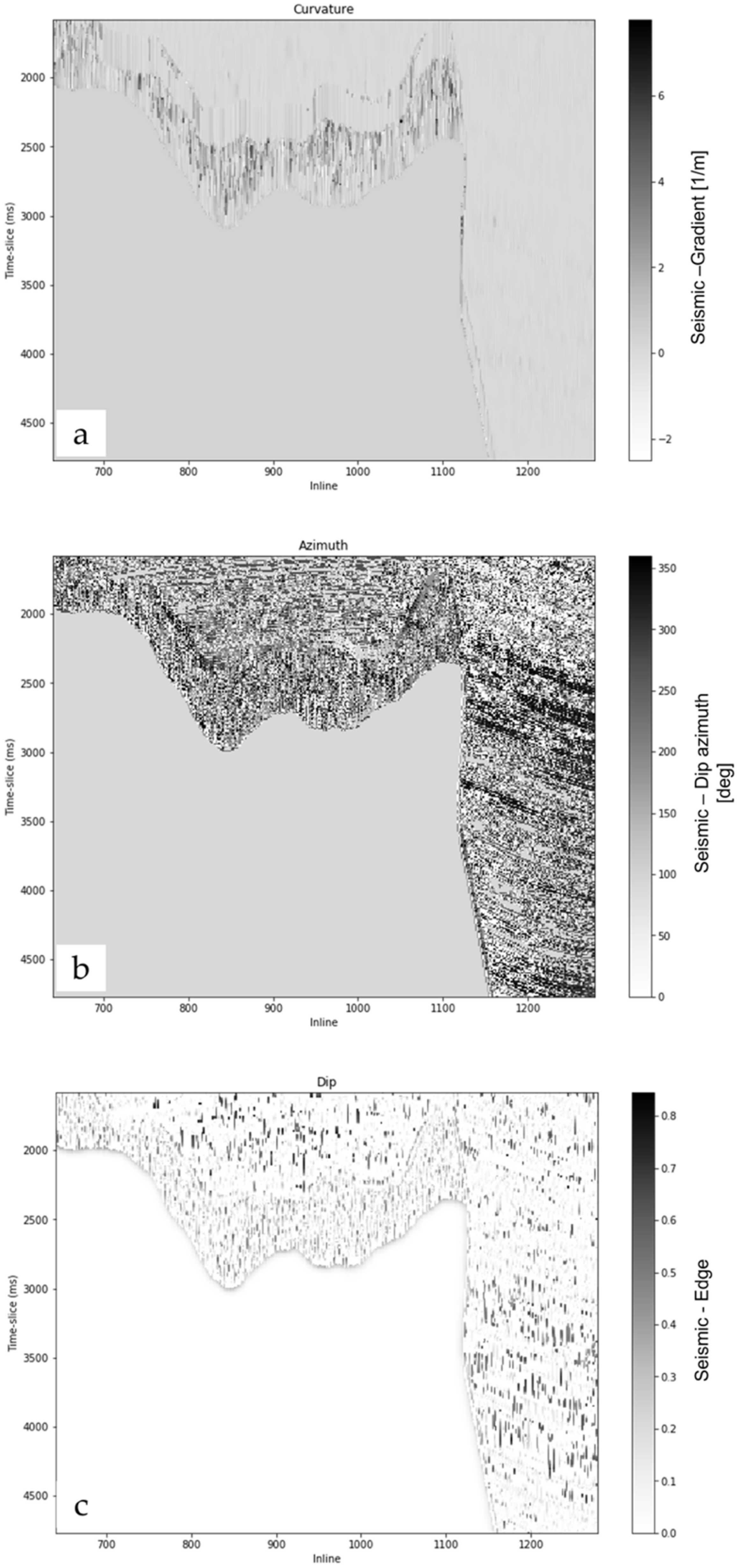
Figure 9 shows the extracted seismic attributes for enhancing the salt delineation, including curvature, azimuth, and dip. The azimuth attribute shows the delineation of salt clearly, while the curvature and dip only show the boundary of the salt region, since the values of salt and background have the same range. The basic statistics of these attributes’ values are present in Table 3.
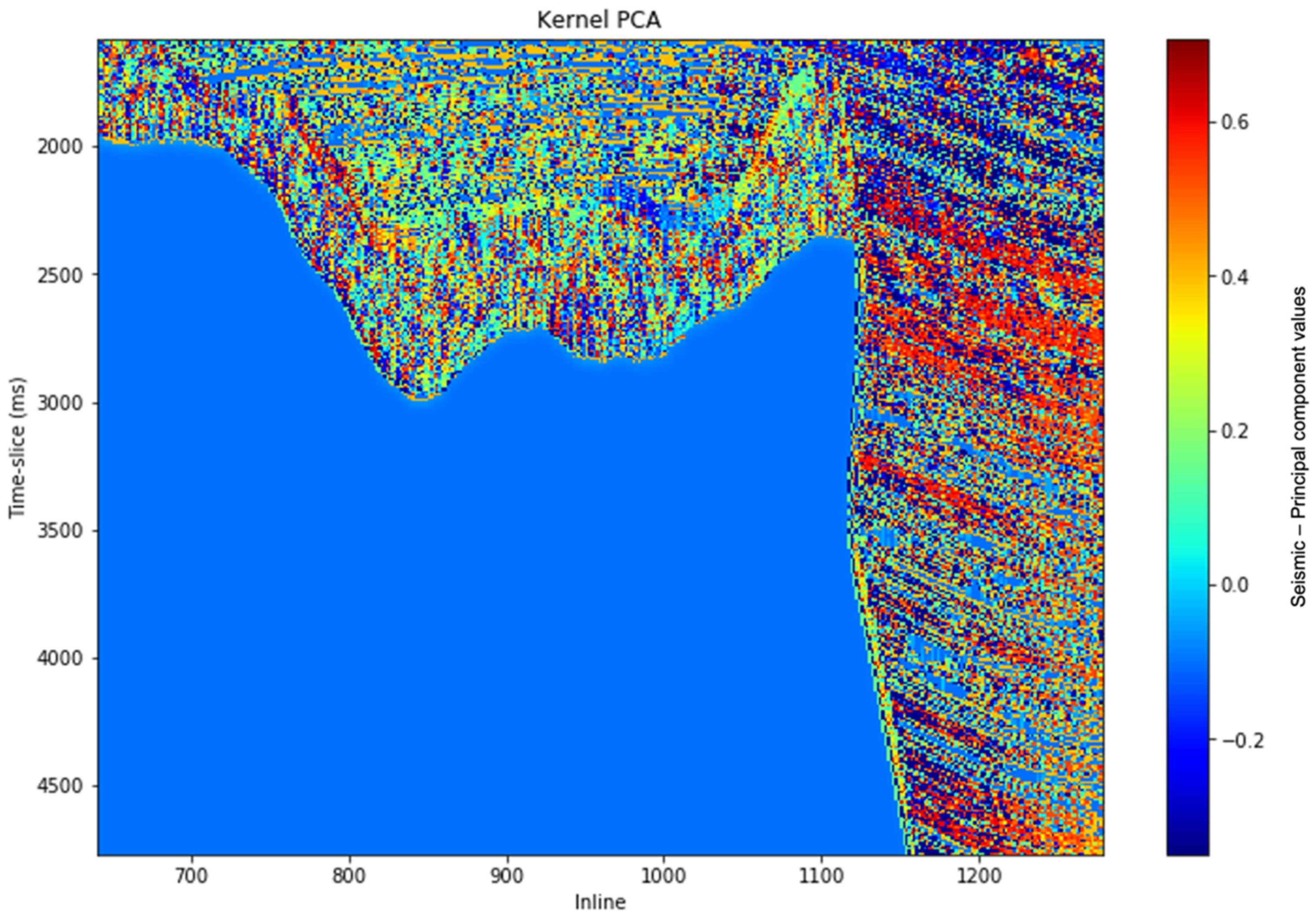
These attributes were then assigned as the input for the dimensionality reduction step. With the KernelPCA algorithm, we tried to transform these three multi-attributes into a single principal component that carried the important information. Figure 10 shows the result of KernelPCA using a linear kernel. The result shows that the KernelPCA can quantify and enhance the salt body and distinguish this geological feature from the background.
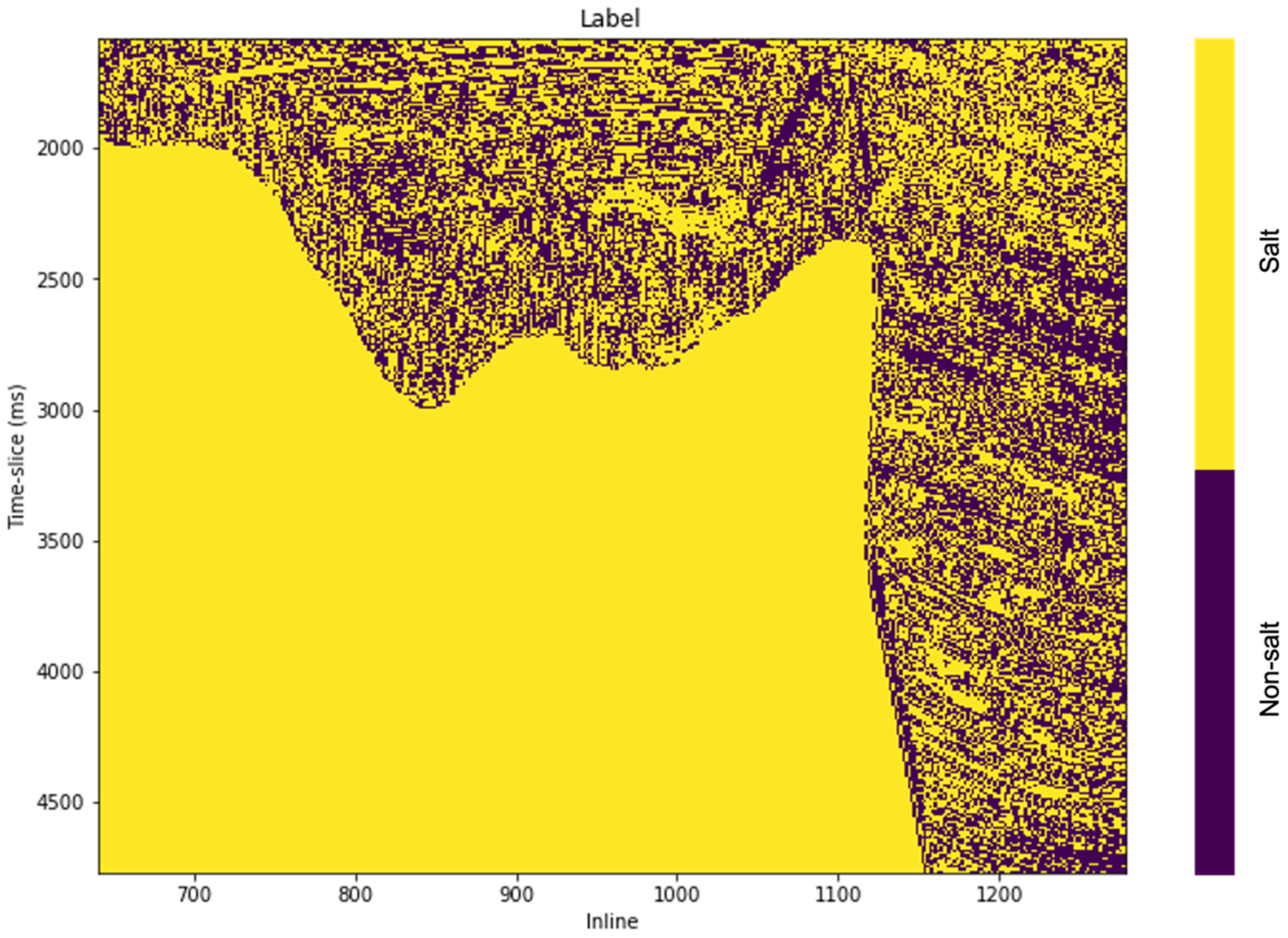
Finally, the output from KernelPCA we assigned as the input for the K-means clustering algorithm. K-means clustering will classify the data into two clusters or binary problems, depending on its values. In this part, we define the cluster into salt features (1) and non-salt or background features (0). The K-means clustering algorithm shows a good result classified those two geological features, but by comparing with the actual interpretation shown in Figure 2, this result is a little noisy on the background features. This occurred as a result of the effect of curvature and dip attributes that provide better differentiation just at the salt boundary, but not within the salt or non-salt region. Nevertheless, this clustering result as shown on Figure 11 will be assigned as the ground truth for the output data.
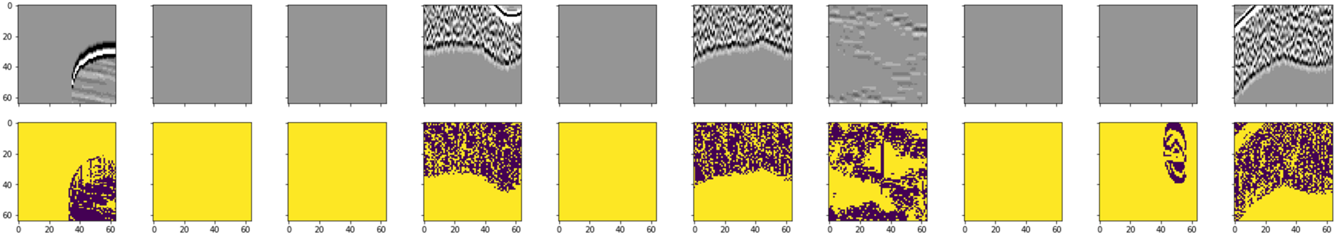
We generate 384 pairs of seismic and ground truth patch data to train the model. The location of those patches is randomized within the original seismic volume. In total, 346 data pairs are assigned as the train data and the rest as the test data. Figure 12 shows the 10 selected data pairs that will be fed into the CNN’s architecture.
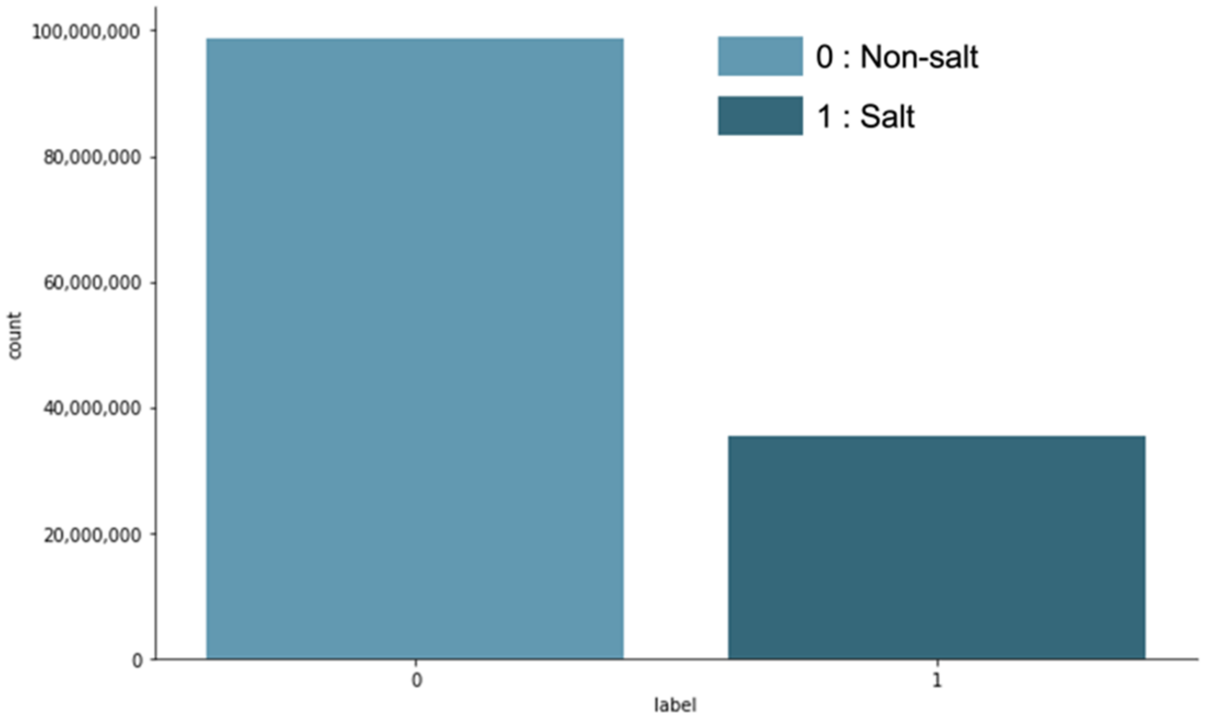
Figure 13 shows the distribution of each label. The graphic shows that salt features dominated the dataset. This unbalanced distribution is supposed to affect the CNN model where the model tends to learn the dominant label; hence, they give a large amount of information to the model.
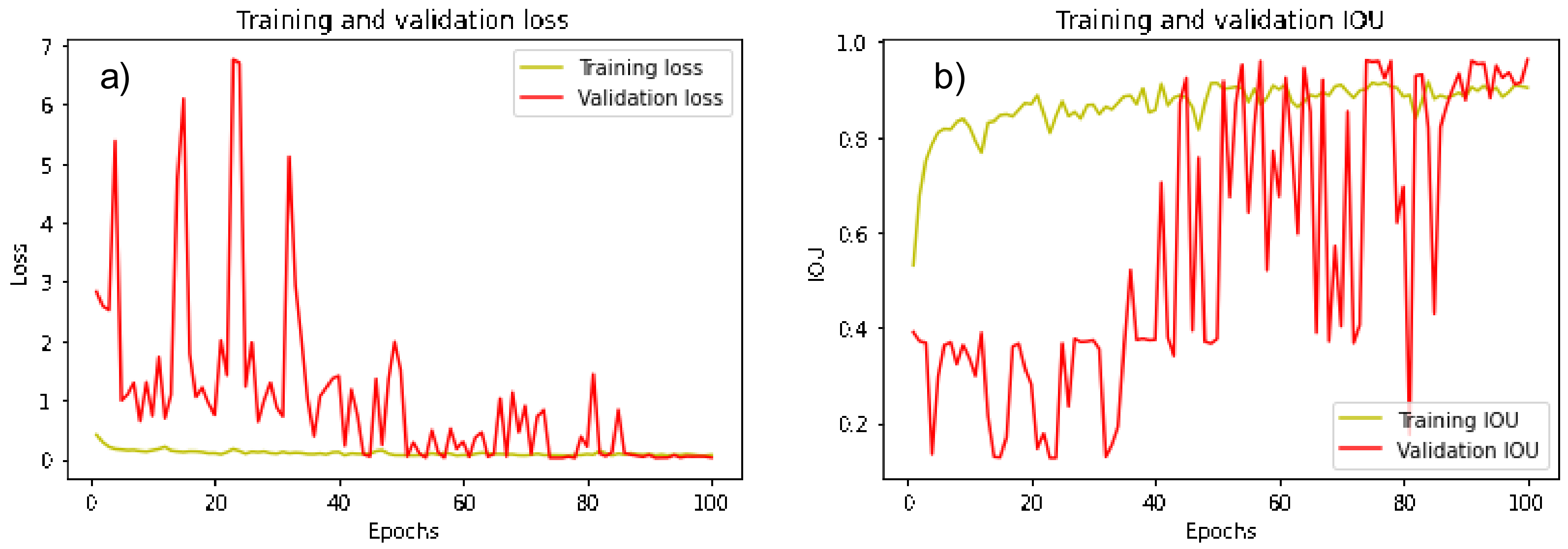
We trained this dataset with a model based on Table 2’s selected parameters. After 30 min of GPU processing time, this model achieved good accuracy for both training and validation data. The model achieved a 0.89 IoU score for the training data and a 0.97 IoU score for the validation data (Figure 14).
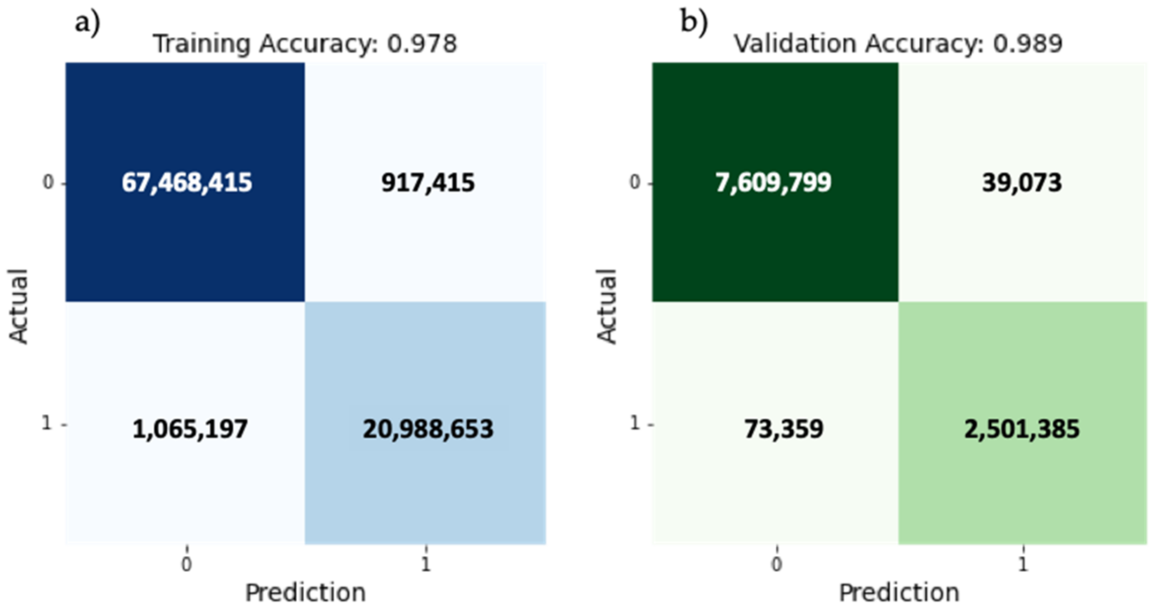
For the confusion matrix, the model successfully achieved a 0.98 F1 score for training data and 0.99 for validation data (Figure 15). Notice that both on the classification report for training and validation data, the salt and non-salt label have relatively the same accuracy. This indicates the robustness of the model, although the dataset is unbalanced. The reason behind this was because we used binary cross entropy as the loss parameter. This loss allocates a higher penalty to minority label samples during the learning process, and it ensures that minority label samples are detected more accurately [47].
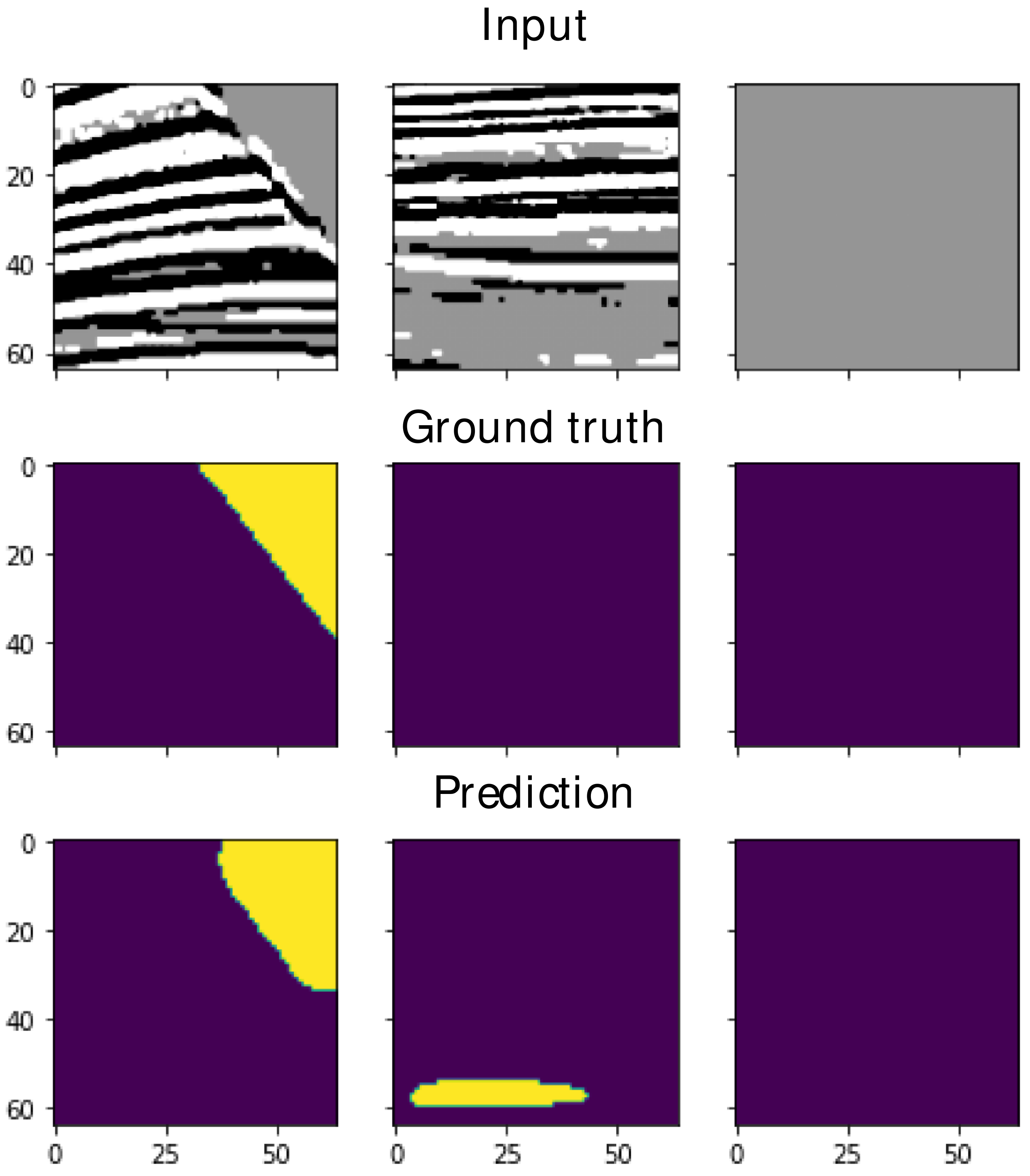
The details of each evaluation metrics including precision, recall, and f1-score for training and validation dataset are shown on the Table 4 and Table 5 respectively. Also, Figure 16 shows the visualization a few examples of random validation data where the top part is the input, the middle part is the ground truth or the true output, and the bottom part is the prediction. This image shows the model successfully detecting the salt feature both for the boundaries and the body. The result of model prediction differs from the ground truth in the middle column, where the model predicted non-layered seismic features such as salt features, but these features are absent on the ground truth.
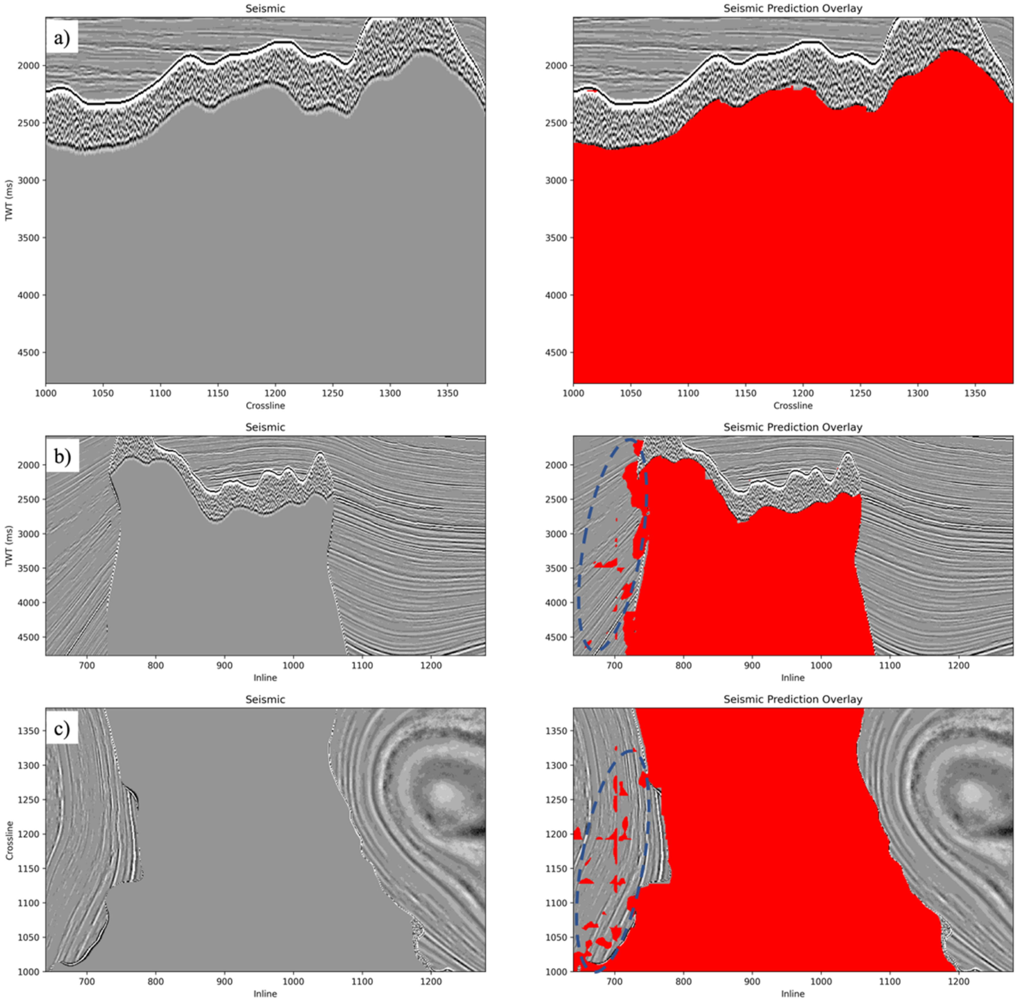
After training the optimum model, we applied this model to the whole seismic data. We divided the entire seismic into 64 × 64 × 64 patches to feed into the model, and then concatenated the predicted patches back into the original size. Figure 17 shows the predicted result with a 2D seismic section display. As we can see, the predicted result gives an outstanding detection of salt bodies on the seismic data. The inline sections (Figure 17a) show the accurate salt feature detection. However, there is also a noisy and misclassified both for crossline and time-slice seismic section (Figure 17b,c).
5.2. The A Field Real Seismic Example
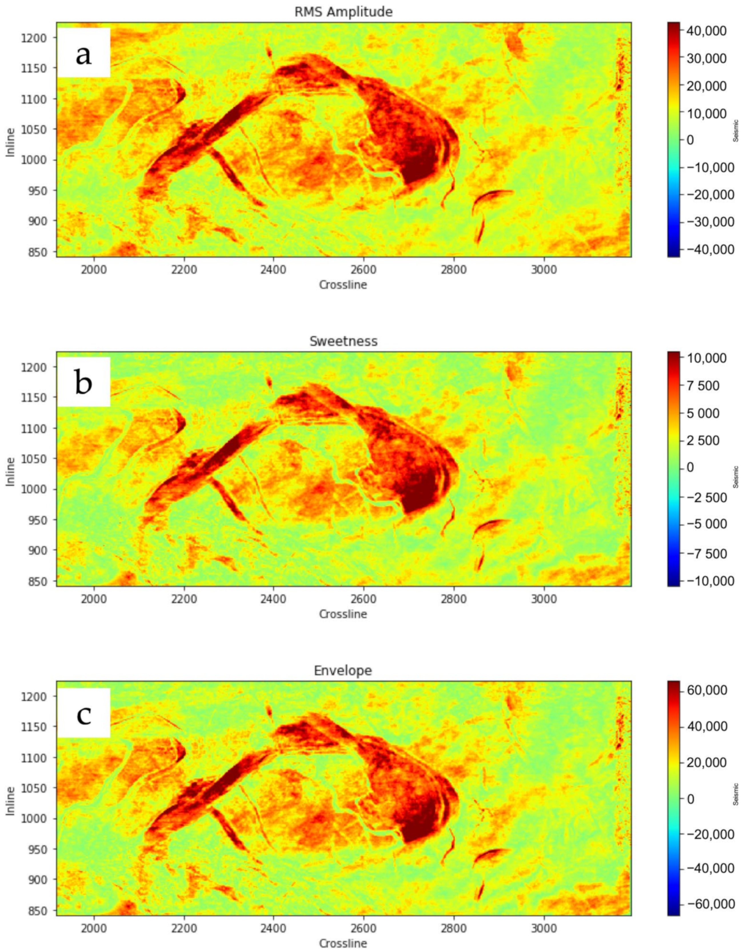
In addition to the synthetic example in the previous part, we further use 3D real seismic data acquired from the A Field in the Malay Basin to verify the generalization of the proposed workflow. We extracted three seismic attributes based on amplitude as the starting point. As shown in Figure 19, these three attributes improve the delineation of channel features, which represent the sand distribution on seismic data, as indicated by the red-coded high value. The sand distribution indicated that the channel-filled deposits were made up of point bar, abandoned channel, crevasse splays, and flood plain [48]. The basic statistics information of the attributes is detailed in Table 6.
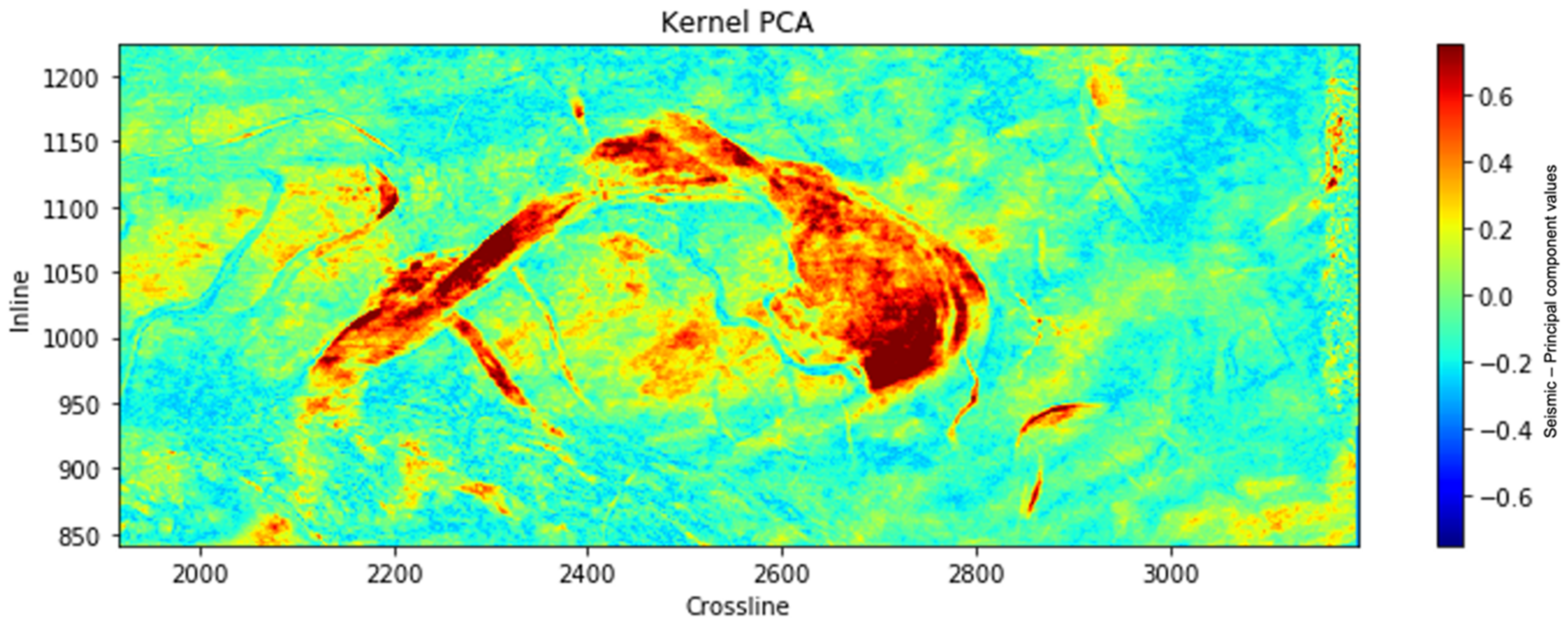
As in the previous example, these attributes are assigned to be the input of the KernelPCA algorithm to transform into a single principal component. The result can be shown in Figure 20. The dimensionality reduction technique helps visualize the meandering of channel features and quantify the channel features. This output can be a good input to the clustering process.
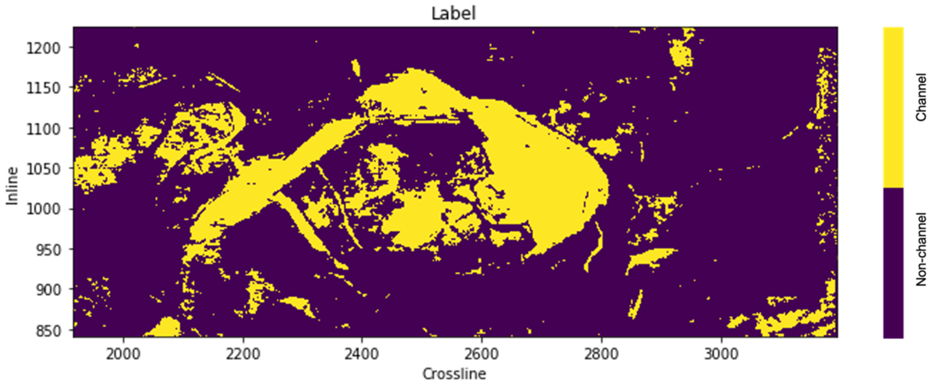
By using these two unsupervised learning techniques i.e., KernelPCA and K-means clustering, we can generate the high resolution of channelized features. Figure 21 shows the classified values, clustered into two geological features, i.e., a (binary) channel and non-channel. This ground truth data are also confirmed by the manual interpretation based on the previous results (Figure 4).
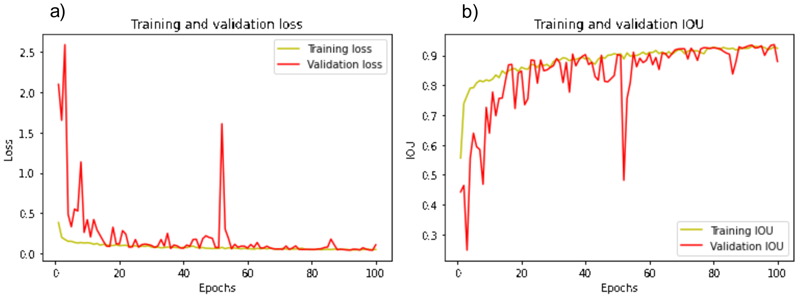
We generated 384 small patch data pairs and assigned 300 data pairs for the training and the rest for the validation. Using 100 epochs to train the model, we achieved 0.84 IoU score on training data and 0.89 IoU score on validation data (Figure 22). The training process takes 32 min in total using the GPU.
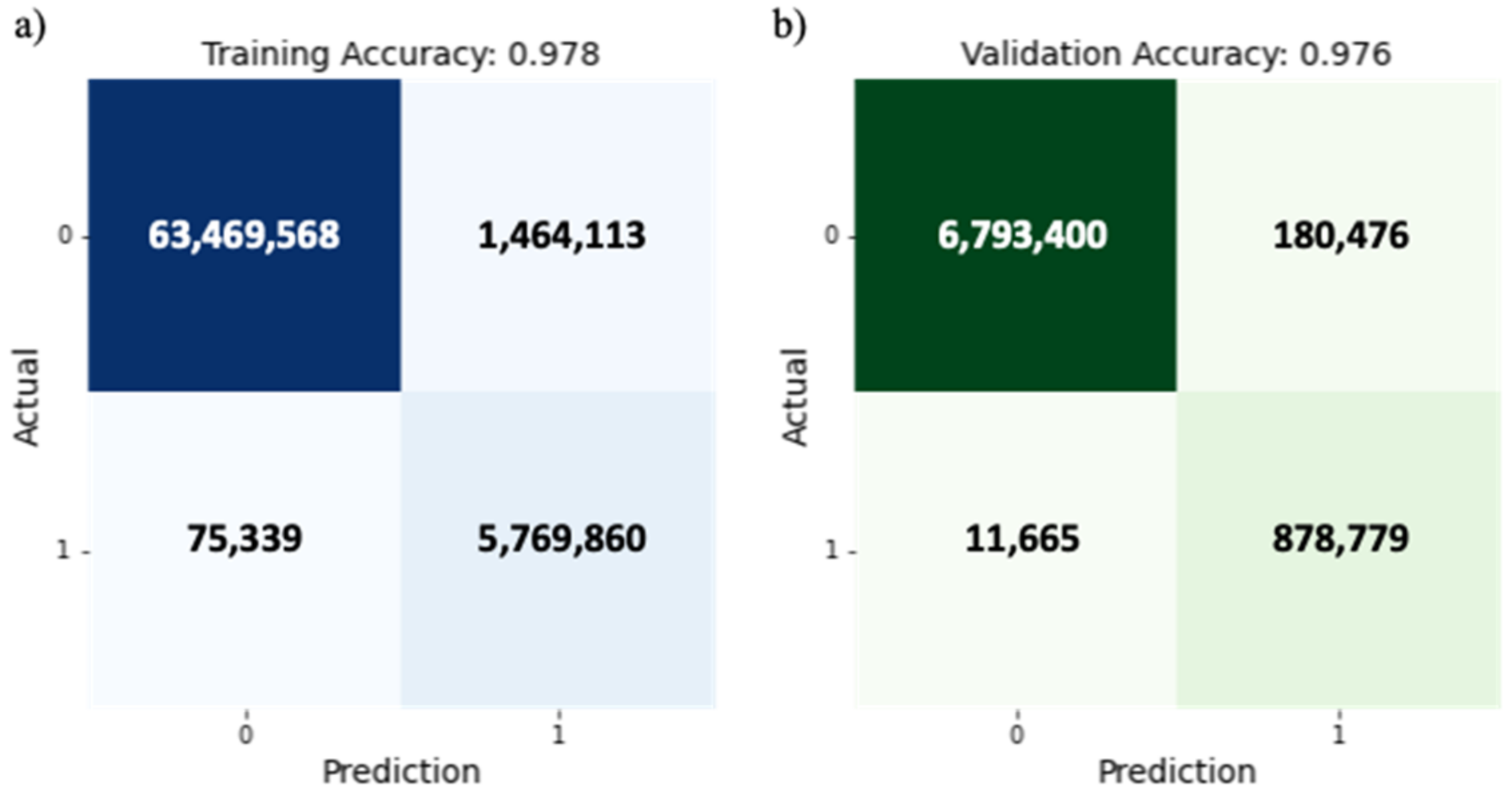
A good result is also obtained by the confusion matrix evaluation. The model obtained 0.98 accuracy score for training and 0.97 for the validation (Figure 23). Table 7 and Table 8 shows the details of evaluation metrics including precision, recall, and f1-score for the training and validation datasets. Although the datasets are imbalanced, the prediction is showing a good accuracy for both the channel and non-channel class.
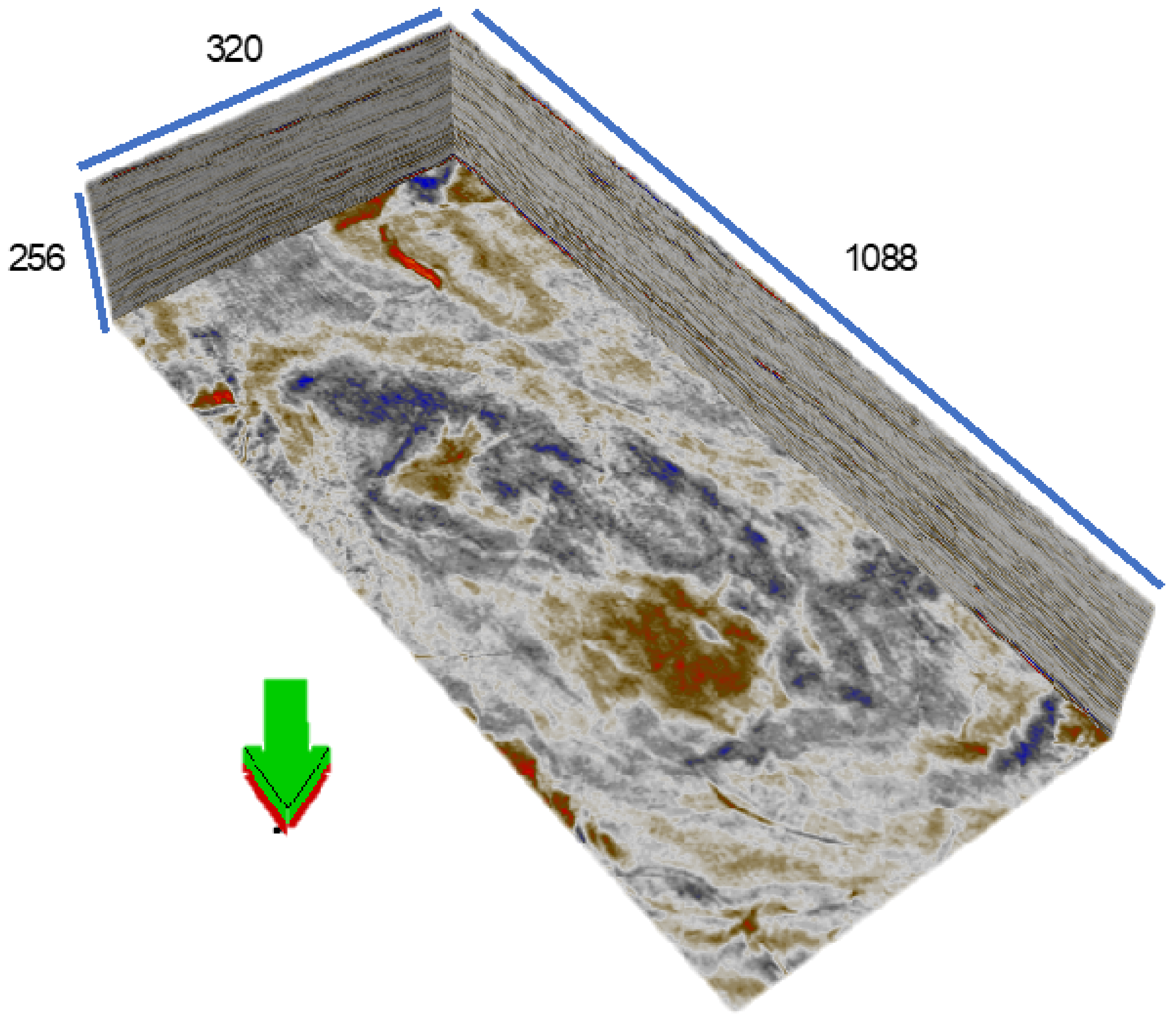
After obtained the optimum model, we applied the model to the whole seismic cube with a size of 320 inline, 1088 crossline, and 256 time-slice (Figure 24). The model shows the accurate detection of the channel features both for the 2D and 3D display.
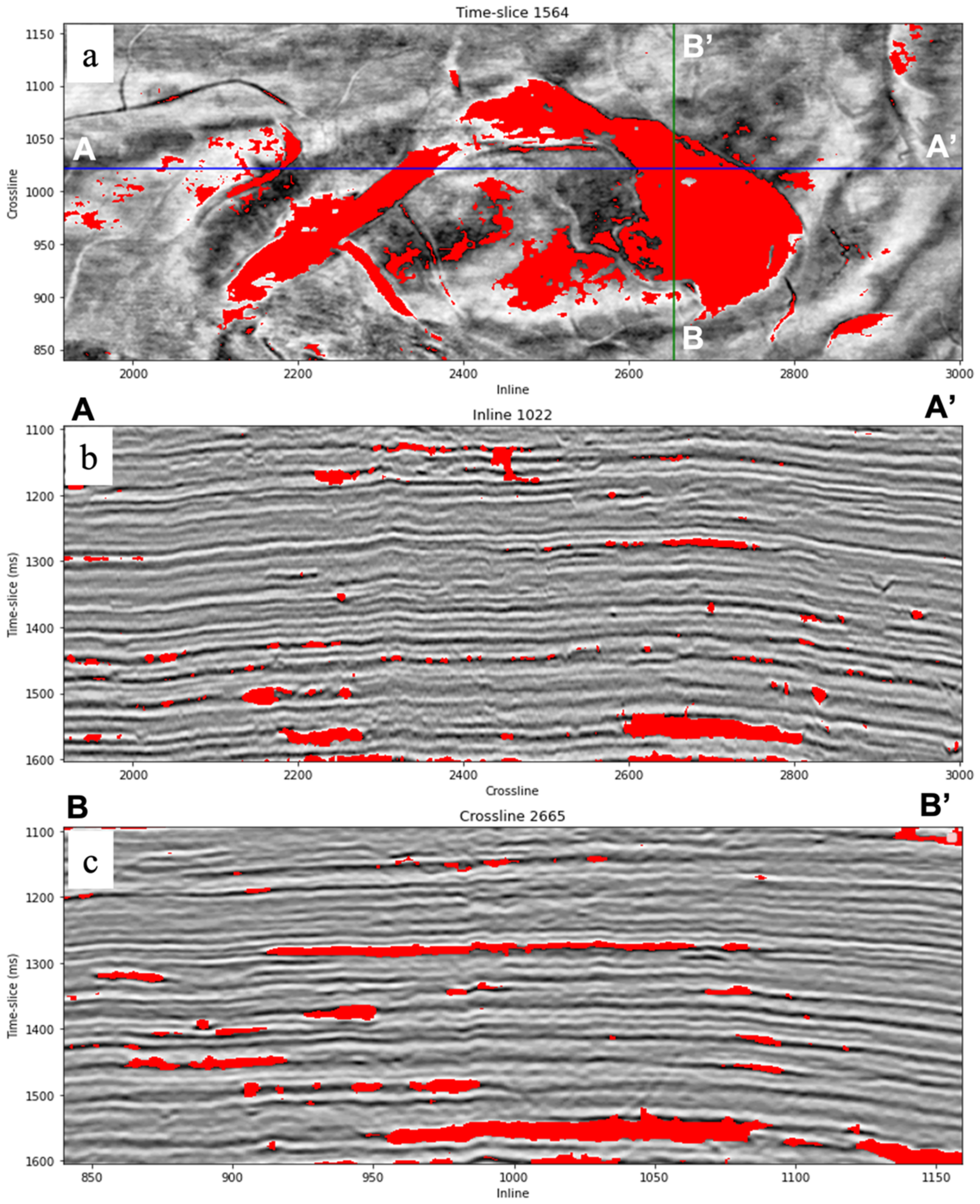
Figure 25 shows the prediction result on the seismic section; the top part is a time-slice in the middle from the inline, and the bottom part on crossline. The channel interpretation is usually performed after time-slice section. The prediction of the CNN model is enhanced and clearly detected the meandering of the channel and channel point bar features. It can also detect the channel features in inline and crossline, where it has only small features.
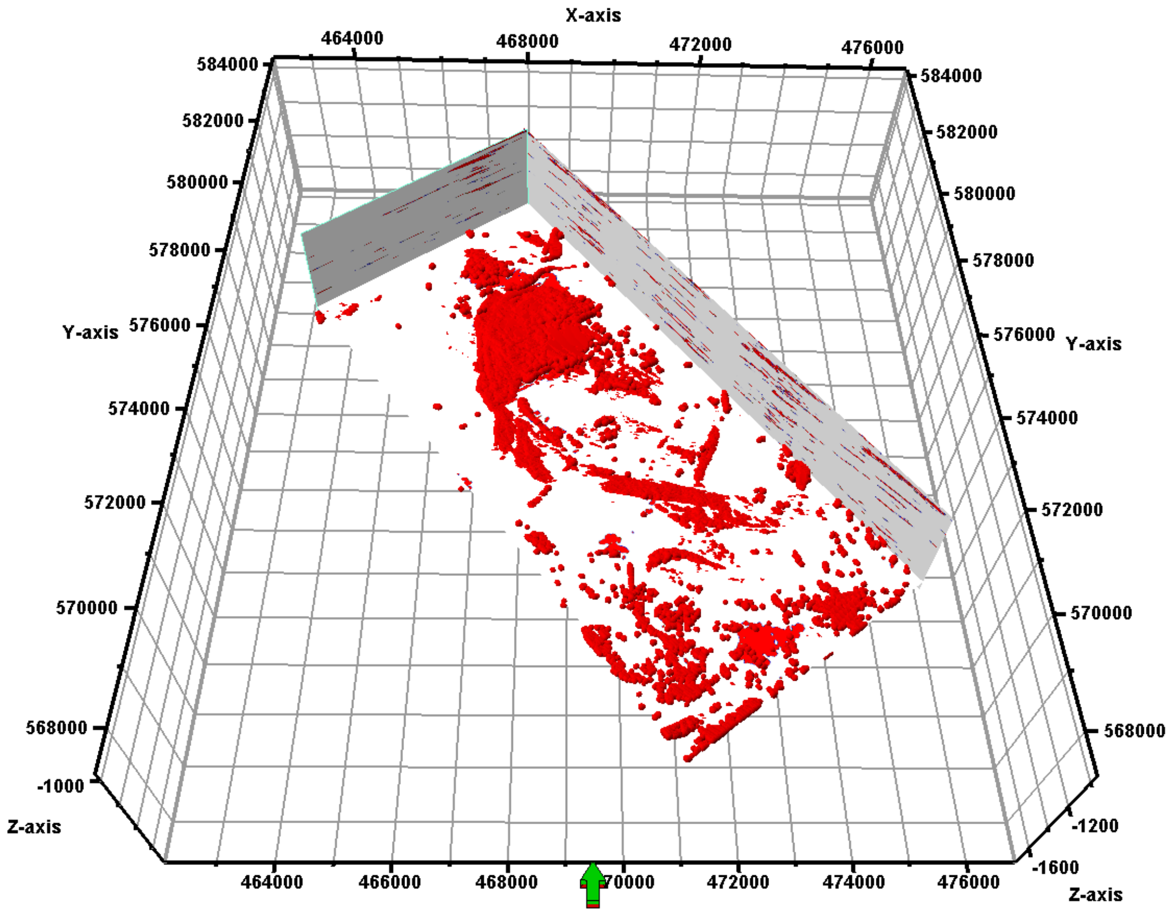
The main advantage to train the model on 3D data is that the model can have spatial and geomorphology information from the object that it wants to detect. Hence, the model gives clear channel body interpretation on the 3D visualization, as shown on the Figure 26.
6. Conclusions
In conclusion, this research successfully detected geological features in seismic data automatically using a semi-supervised learning technique. We combine unsupervised learning to generate the label data using a proposed workflow and supervised learning to build a model for geological feature detection.
The main problem of applying deep learning-based techniques to geoscience problems is the lack of label data for the training process, since it is a subjective and time-consuming task. To address this problem, we used the proposed workflow to generate numerous label datasets for training the model. This workflow starts with seismic attribute extraction to help enhance the visualization of the targeted geological features. Then, we applied KernelPCA to transform those multi-attributes into single principal components, and finally, we used K-means clustering to classify the geological label into binary classes.
We consider this geological detection one of the image segmentation problems. We used one of CNN’s architectures, namely U-Net, to build the model. The U-Net architecture was originally proposed for 2D medical purposes. We modified this architecture to fit the geological detection problem by tuning the hyperparameters, including changing the architecture and applying the transfer learning technique.
We apply this semi-supervised learning technique to synthetic and real seismic 3D datasets with vastly different geological settings to validate it. The synthetic data are from the SEAM dataset, which is a salt-dominated field, and the real data are from a case study from the Malay Basin, which is interpreted as a meandering fluvial reservoir. The application of two dataset examples demonstrated that the trained model is accurate and consistent with manual interpretations. With the model prediction result, we were able to automatically extract the 3D body of the geological target. Furthermore, this model could help the interpreter focus on the task that needs human expertise and help the model obtain better detection and prediction results.
Author Contributions
Conceptualization, H.P. and A.H.A.L.; methodology, H.P.; software, H.P.; validation, H.P. and A.H.A.L.; formal analysis, H.P. and A.H.A.L.; investigation, H.P. and A.H.A.L.; resources, H.P. and A.H.A.L.; data curation, H.P. and A.H.A.L.; writing—original draft preparation, H.P.; writing—review and editing, H.P. and A.H.A.L.; visualization, H.P.; supervision, A.H.A.L. All authors have read and agreed to the published version of the manuscript.
Funding
This research was funded by the UTP 3D true-amplitude target-oriented migration (015MD0-076).
Institutional Review Board Statement
Not applicable.
Informed Consent Statement
Not applicable.
Data Availability Statement
The SEAM synthetic datasets were analyzed in this study is publicly available datasets. This data can be found here: [https://seg.org/SEAM/open-data].
Acknowledgments
The authors would like to thank SEG Advanced Modeling for providing the open dataset. Also, PETRONAS Malaysia and the Centre for Subsurface Imaging UTP for providing the data for this study. We would like to express our appreciation to the Centre for Subsurface Imaging and our colleagues at the Geoscience department of Universiti Teknologi PETRONAS for supporting us throughout the project. Huge gratitude is extended to the UTP 3D true-amplitude target-oriented migration project with cost center 015MD0-076 for granting this research. We acknowledge the Schlumberger Company for providing Petrel software licensing.
Conflicts of Interest
The authors declare no conflict of interest.
Abbreviations
| 3D | Three-Dimensional |
| CNN | Convolutional Neural Network |
| FN | False Negative |
| FP | False Positive |
| GPU | Graphics Processing Unit |
| IoU | Intersection over Union |
| NW | Northwest |
| PCA | Principal Component Analysis |
| RMS | Root Mean Square |
| SE | Southeast |
| SOM | Self-Organizing Maps |
| SVM | Support Vector Machine |
| TN | True Negative |
| TP | True Positive |
References
- Barnes, A.E. Handbook of Poststack Seismic Attributes; Society of Exploration Geophysicists: Houston, TX, USA, 2016. [Google Scholar]
- Lines, L.R.; Newrick, R.T. Fundamentals of Geophysical Interpretation; Society of Exploration Geophysicists: Houston, TX, USA, 2004. [Google Scholar]
- Zhao, T.; Verma, S.; Qi, J.; Marfurt, K.J. Supervised and Unsupervised Learning: How Machines Can Assist Quantitative Seismic Interpretation. In SEG Technical Program Expanded Abstracts; Society of Exploration Geophysicists: Houston, TX, USA, 2015. [Google Scholar]
- Waldeland, A.U.; Jensen, A.C.; Gelius, L.-J.; Solberg, A.H.S. Convolutional Neural Networks for Automated Seismic Interpretation. Lead. Edge 2018, 37, 482–560. [Google Scholar] [CrossRef]
- Zhang, Y.X.; Liu, Y.; Zhang, H.R.; Xue, H. Automatic Salt Dome Detection Using U-Net. In Proceedings of the 81st EAGE Conference and Exhibition 2019, London, UK, 3–6 June 2019. [Google Scholar]
- Shi, Y.; Wu, X.; Fomel, S. Automatic Salt-Body Classification Using a Deep Convolutional Neural Network. In Proceedings of the 2018 SEG International Exposition and Annual Meeting, SEG 2018, Anaheim, CA, USA, 14–19 October 2018. [Google Scholar]
- Wu, X.; Liang, L.; Shi, Y.; Fomel, S. FaultSeg3D: Using Synthetic Data Sets to Train an End-to-End Convolutional Neural Network for 3D Seismic Fault Segmentation. Geophysics 2019, 84, IM35–IM45. [Google Scholar] [CrossRef]
- Araya-Polo, M.; Dahlke, T.; Frogner, C.; Zhang, C.; Poggio, T.; Hohl, D. Automated Fault Detection without Seismic Processing. Lead. Edge 2017, 36, 208–214. [Google Scholar] [CrossRef]
- Wrona, T.; Pan, I.; Gawthorpe, R.L.; Fossen, H. Seismic Facies Analysis Using Machine Learning. Geophysics 2018, 83, 83–95. [Google Scholar] [CrossRef]
- Zhao, T. Seismic Facies Classification Using Different Deep Convolutional Neural Networks. In Proceedings of the 2018 SEG International Exposition and Annual Meeting, SEG 2018, Anaheim, CA, USA, 14–19 October 2018. [Google Scholar]
- Alaudah, Y.; Michałowicz, P.; Alfarraj, M.; AlRegib, G. A Machine-Learning Benchmark for Facies Classification. Interpretation 2019, 7, SE175–SE187. [Google Scholar] [CrossRef] [Green Version]
- Dramsch, J.S.; Lüthje, M. Deep Learning Seismic Facies on State-of-the-Art CNN Architectures. In Proceedings of the 2018 SEG International Exposition and Annual Meeting, SEG 2018, Anaheim, CA, USA, 14–19 October 2018. [Google Scholar]
- Chopra, S.; Marfurt, K.J. Unsupervised Machine Learning Applications for Seismic Facies Classification. In Proceedings of the SPE/AAPG/SEG Unconventional Resources Technology Conference 2019, URTC 2019, Denver, CO, USA, 22–24 July 2019. [Google Scholar]
- Troccoli, E.B.; Cerqueira, A.G.; Lemos, J.B.; Holz, M. K-Means Clustering Using Principal Component Analysis to Automate Label Organization in Multi-Attribute Seismic Facies Analysis. J. Appl. Geophys. 2022, 198, 104555. [Google Scholar] [CrossRef]
- Galvis, I.S.; Villa, Y.; Duarte, C.; Sierra, D.; Agudelo, W. Seismic Attribute Selection and Clustering to Detect and Classify Surface Waves in Multicomponent Seismic Data by Using k-Means Algorithm. Lead. Edge 2017, 36, 194–280. [Google Scholar] [CrossRef]
- Zhao, T.; Zhang, J.; Li, F.; Marfurt, K.J. Characterizing a Turbidite System in Canterbury Basin, New Zealand, Using Seismic Attributes and Distance-Preserving Self-Organizing Maps. Interpretation 2016, 4, SB79–SB89. [Google Scholar] [CrossRef] [Green Version]
- Puzyrev, V.; Elders, C. Deep Convolutional Autoencoder for Unsupervised Seismic Facies Classification. In Proceedings of the EAGE/AAPG Digital Subsurface for Asia Pacific Conference 2020, Online. 7–10 September 2020. [Google Scholar]
- Ronneberger, O.; Fischer, P.; Brox, T. U-Net: Convolutional Networks for Biomedical Image Segmentation. In Proceedings of the Medical Image Computing and Computer-Assisted Intervention—MICCAI 2015, Munich, Germany, 5–9 October 2015. [Google Scholar] [CrossRef] [Green Version]
- Jervis, M.; Liu, M.; Smith, R. Deep Learning Network Optimization and Hyperparameter Tuning for Seismic Lithofacies Classification. Lead. Edge 2021, 40, 514. [Google Scholar] [CrossRef]
- Rezende, E.; Ruppert, G.; Carvalho, T.; Ramos, F.; De Geus, P. Malicious Software Classification Using Transfer Learning of ResNet-50 Deep Neural Network. In Proceedings of the 16th IEEE International Conference on Machine Learning and Applications, ICMLA 2017, Cancun, Mexico, 18–21 December 2017. [Google Scholar]
- Fehler, M.; Keliher, P.J. SEAM Phase 1: Challenges of Subsalt Imaging in Tertiary Basins, with Emphasis on Deepwater Gulf of Mexico; Society of Exploration Geophysicists: Houston, TX, USA, 2011. [Google Scholar]
- Madon, M.; Abolins, P.; Hassan, R.A.; Yakzan, A.M.; Yang, J.-S.; Zainal, S.B. Petroleum Systems of the North Malay Basin. Bull. Geol. Soc. Malays. 2004, 49, 125–134. [Google Scholar] [CrossRef] [Green Version]
- Bishop, M.G. Petroleum Systems of the Malay Basin Province, Malaysia; U.S. Geological Survey: Reston, VA, USA, 2002.
- Lin, L.; Ismail, H.; Abdul Kadir, M.F.; Tajuddin, M. Stratal Slicing: A Tool for Imaging Geologically Time-Equivalent Fluvial Architecture—A Field Case Study. In Proceedings of the International Petroleum Technology Conference, Bangkok, Thailand, 14–16 November 2016. [Google Scholar]
- Miall, A.D. Architectural-Element Analysis: A New Method of Facies Analysis Applied to Fluvial Deposits. Earth Sci. Rev. 1985, 22, 261–308. [Google Scholar] [CrossRef]
- Brown, A.R. Understanding Seismic Attributes. Geophysics 2001, 66, 47. [Google Scholar] [CrossRef]
- Ghosh, D.; Sajid, M.; Ibrahim, N.A.; Viratno, B. Seismic Attributes Add a New Dimension to Prospect Evaluation and Geomorphology Offshore Malaysia. Lead. Edge 2014, 33, 477–588. [Google Scholar] [CrossRef]
- Shahman, N.S.; Anuar, N.; Elsaadany, M.; Ghosh, D.P. Seismic Attributes for Enhancing Structural and Stratigraphic Features: Application to N-Field, Malay Basin, Malaysia. Bull. Geol. Soc. Malays. 2021, 72, 101–111. [Google Scholar] [CrossRef]
- Fossen, H. Structural Geology; Cambridge University Press: Cambridge, UK, 2016. [Google Scholar]
- Clausolles, N.; Collon, P.; Caumon, G. Generating Variable Shapes of Salt Geobodies from Seismic Images and Prior Geological Knowledge. Interpretation 2019, 7, T829. [Google Scholar] [CrossRef]
- Posamentier, H.W.; Davies, R.J.; Cartwright, J.A.; Wood, L.J. (Eds.) Seismic Geomorphology—An Overview. In Seismic Geomorphology: Applications to Hydrocarbon Exploration and Production; The Geological Society of London: London, UK, 2007. [Google Scholar]
- Babikir, I.A.M.; Salim, A.M.A.; Ghosh, D.P. Stratigraphic characterization of a fluvial reservoir using seismic attributes and spectral decomposition: An example from the Northern Malay Basin. Pet. Coal 2018, 60, 943–950. [Google Scholar]
- Hazmi Abdul Malik, M.; Shyh Zung, L. Application of Seismic Attribute and Spectral Decomposition: Example of Fluvial System During Miocene in Field A., Malay Basin. J. Eng. Appl. Sci. 2019, 14, 1110–1121. [Google Scholar] [CrossRef] [Green Version]
- Sun, X.; Sun, S.Z.; Tian, J.; Han, J. Sparse Kernel Principal Component Analysis on Seismic Denoising and Fluid Identification. In Proceedings of the 75th European Association of Geoscientists and Engineers Conference and Exhibition 2013 Incorporating SPE EUROPEC 2013: Changing Frontiers, London, UK, 10–13 June 2013. [Google Scholar]
- Yin, X.Y.; Kong, G.Y.; Zhang, G.Z. Seismic Attributes Optimization Based on Kernel Principal Component Analysis (KPCA) and Application. Shiyou Diqiu Wuli Kantan/Oil Geophys. Prospect. 2008, 43, 179–183. [Google Scholar]
- Vapnik, V. The Support Vector Method of Function Estimation. In Nonlinear Modeling; Springer: New York, NY, USA, 1998. [Google Scholar]
- Calvin, L.D.; LeCam, L.; Neyman, J. Proceedings of the Fifth Berkeley Symposium on Mathematical Statistics and Probability, Volume V, Weather Modification. J. Am. Stat. Assoc. 1969, 64, 1085–1087. [Google Scholar] [CrossRef]
- Duan, Y.; Zheng, X.; Hu, L.; Sun, L. Seismic Facies Analysis Based on Deep Convolutional Embedded Clustering. Geophysics 2019, 84, IM87. [Google Scholar] [CrossRef]
- Haraty, R.A.; Dimishkieh, M.; Masud, M. An Enhanced K-Means Clustering Algorithm for Pattern Discovery in Healthcare Data. Int. J. Distrib. Sens. Netw. 2015, 2015, 1–11. [Google Scholar] [CrossRef]
- Civitarese, D.; Szwarcman, D.; Brazil, E.V.; Zadrozny, B. Semantic Segmentation of Seismic Images. arXiv 2019, arXiv:1905.04307. [Google Scholar]
- Lecun, Y.; Bengio, Y.; Hinton, G. Deep Learning. Nature 2015, 521, 436–444. [Google Scholar] [CrossRef] [PubMed]
- Enyinna Nwankpa, C.; Ijomah, W.; Gachagan, A.; Marshall, S. Activation Functions: Comparison of Trends in Practice and Research for Deep Learning. arXiv 2018, arXiv:1811.03378. [Google Scholar]
- Kingma, D.P.; Lei Ba, J. Adam: A method for stochastic optimization. arXiv 2014, arXiv:1412.6980. [Google Scholar]
- Russakovsky, O.; Deng, J.; Su, H.; Krause, J.; Satheesh, S.; Ma, S.; Huang, Z.; Karpathy, A.; Khosla, A.; Bernstein, M.; et al. ImageNet Large Scale Visual Recognition Challenge. Int. J. Comput. Vis. 2015, 115, 211–252. [Google Scholar] [CrossRef] [Green Version]
- Ting, K.M. Confusion Matrix. In Encyclopedia of Machine Learning and Data Mining; Springer Science and Business Media: New York, NY, USA, 2017. [Google Scholar]
- Rezatofighi, H.; Tsoi, N.; Gwak, J.; Sadeghian, A.; Reid, I.; Savarese, S. Generalized Intersection over Union: A Metric and a Loss for Bounding Box Regression. In Proceedings of the Proceedings of the IEEE Computer Society Conference on Computer Vision and Pattern Recognition, Long Beach, CA, USA, 15–20 June 2019. [Google Scholar]
- Rezaei-Dastjerdehei, M.R.; Mijani, A.; Fatemizadeh, E. Addressing Imbalance in Multi-Label Classification Using Weighted Cross Entropy Loss Function. In Proceedings of the 27th National and 5th International Iranian Conference of Biomedical Engineering, ICBME 2020, Tehran, Iran, 26–27 November 2020. [Google Scholar]
- Hossain, S. Application of Seismic Attribute Analysis in Fluvial Seismic Geomorphology. J. Pet. Explor. Prod. Technol. 2020, 10, 1009–1019. [Google Scholar] [CrossRef] [Green Version]
Figure 1.
The velocity model cross section.

Figure 2.
The salt features based on velocity values on the model cross section.

Figure 3.
The location of A Field.

Figure 4.
Interpreted model of the fluvial depositional elements map.

Figure 5.
The proposed workflow of automatic geological features detection using semi-supervised learning.
Figure 5.
The proposed workflow of automatic geological features detection using semi-supervised learning.

Figure 6.
Process of creating small patches from (a) original seismic input volume with 1408 × 1408 × 640 size and (b) ground truth output volume with 64 × 64 × 64 size.
Figure 6.
Process of creating small patches from (a) original seismic input volume with 1408 × 1408 × 640 size and (b) ground truth output volume with 64 × 64 × 64 size.

Figure 7.
The modified U-Net architecture: decreased number of filters on encoder path and increased number of filters on decoder part.
Figure 7.
The modified U-Net architecture: decreased number of filters on encoder path and increased number of filters on decoder part.

Figure 8.
SEAM 3D synthetic data.

Figure 9.
The extracted seismic attributes for salt delineation including (a) curvature, (b) azimuth, and (c) dip.
Figure 9.
The extracted seismic attributes for salt delineation including (a) curvature, (b) azimuth, and (c) dip.

Figure 10.
The KernelPCA result of reducing the multi-attributes for salt delineation analysis.

Figure 11.
The labeled data based on the K-means clustering result.

Figure 12.
Example of the pairs that assigned as input (top) and output (bottom) data.

Figure 13.
The labels’ distribution.

Figure 14.
Training and validation (a) loss and (b) accuracy.

Figure 15.
The confusion matrix of (a) training and (b) validation data.

Figure 16.
The predicted result on the validation data.

Figure 17.
The predicted result of salt features on (a) inline, (b) crossline, and (c) time-slice seismic section.
Figure 17.
The predicted result of salt features on (a) inline, (b) crossline, and (c) time-slice seismic section.

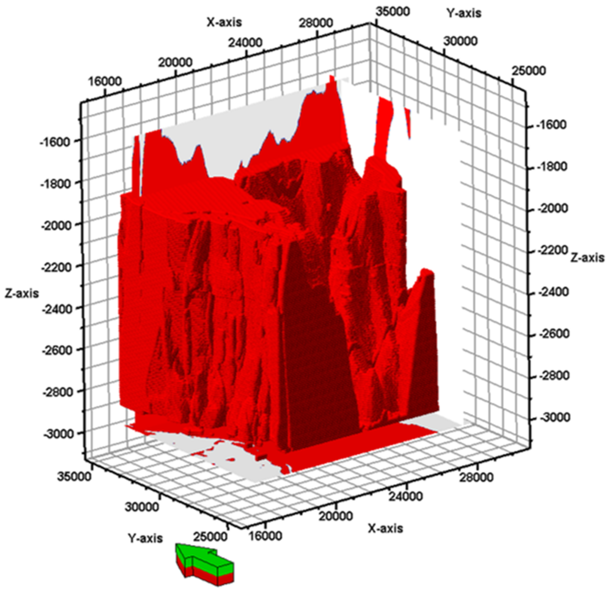
Figure 18.
The predicted result of a salt body in 3D cube visualization.

Figure 19.
The extracted attributes for channel delineation including (a) RMS Amplitude, (b) envelope, and (c) sweetness.
Figure 19.
The extracted attributes for channel delineation including (a) RMS Amplitude, (b) envelope, and (c) sweetness.

Figure 20.
The result of dimensionality reduction using KernelPCA.

Figure 21.
The ground truth data, generated from the clustering result.

Figure 22.
The result of training and validation (a) loss and (b) accuracy.

Figure 23.
The confusion matrix of (a) training data and (b) validation data.

Figure 24.
The 3D real seismic data, acquired from the A Field, Malay Basin.

Figure 25.
The predicted result of channel features on (a) time-slice, (b) inline, and (c) crossline seismic section.
Figure 25.
The predicted result of channel features on (a) time-slice, (b) inline, and (c) crossline seismic section.

Figure 26.
The predicted channel features on 3D data.


Table 1.
Seismic attributes with key seismic properties and the geological applications.
| Seismic Attributes | Seismic Properties | Geological Features |
|---|---|---|
| Reflection Strength | Amplitude | Channels, bright spots, and stratigraphy |
| RMS Amplitude | Amplitude | Channels, bright spots, and stratigraphy |
| Sweetness | Amplitude | Channels, bright spots, and stratigraphy |
| Envelope | Amplitude | Channels, bright spots, and stratigraphy |
| Average Frequency | Frequency | Shadows and stratigraphy |
| Bandwidth | Frequency | Shadows and stratigraphy |
| Tuning Frequency | Frequency | Shadows and stratigraphy |
| Instantaneous Phase | Phase | Faults, salts, and stratigraphy |
| Response Phase | Phase | Faults, salts, and stratigraphy |
Table 2.
Selected hyperparameters.
| Parameter | Selection |
|---|---|
| Architecture | U-Net |
| Encoder Weights | Resnet50 |
| Number of Channels | 3 (1 stacked into 3) |
| Number of Output | Two (geological features and background) |
| Activation | Sigmoid |
| Patch Size | 64 × 64 × 64 |
| Learning Rate | 0.0001 |
| Optimization | Adam |
| Metrics | IOU Score |
| Loss | Binary Focal Dice Loss |
| Batch Size | 16 |
| Epochs | 100 |
Table 3.
The basic statistic of salt delineation seismic attributes.
| Attribute | Count | Mean | Std | Min | 25% | 50% | 75% | Max |
|---|---|---|---|---|---|---|---|---|
| Curvature | 78,643,200 | 0.28 | 0.41 | −5.45 | 0.05 | 0.33 | 0.33 | 10.00 |
| Azimuth | 78,643,200 | 122.44 | 79.36 | 0.00 | 90.00 | 90.00 | 161.57 | 360.00 |
| Dip | 78,643,200 | 0.04 | 0.11 | 0.00 | 0.00 | 0.00 | 0.00 | 0.93 |
Table 4.
The classification report for the training process on synthetic seismic data.
| Class | Precision | Recall | F1-Score | Support |
|---|---|---|---|---|
| non-salt | 0.98 | 0.99 | 0.99 | 68,385,830 |
| salt | 0.96 | 0.95 | 0.95 | 22,053,850 |
Table 5.
The classification report for validation data on synthetic seismic data.
| Class | Precision | Recall | F1-Score | Support |
|---|---|---|---|---|
| non-salt | 0.99 | 0.99 | 0.99 | 7,648,872 |
| salt | 0.98 | 0.97 | 0.98 | 2,574,744 |
Table 6.
The basic statistic information of seismic amplitude attributes.
| Attribute | Count | Mean | Std | Min | 25% | 50% | 75% | Max |
|---|---|---|---|---|---|---|---|---|
| RMS Amplitude | 31,457,280 | 13047.69 | 6902.03 | 0.00 | 8269.11 | 11,525.32 | 16,103.23 | 70,431.49 |
| Sweetness | 31,457,280 | 2671.39 | 1680.15 | 0.00 | 1508.40 | 2355.61 | 3412.71 | 18,976.22 |
| Envelope | 31,457,280 | 17653.89 | 11064.69 | 0.00 | 9692.74 | 15,506.27 | 22,638.18 | 110,397.98 |
Table 7.
The classification report for the training process on real seismic data.
| Class | Precision | Recall | F1-score | Support |
|---|---|---|---|---|
| non-channel | 1.00 | 0.98 | 0.99 | 64,933,681 |
| channel | 0.80 | 0.99 | 0.88 | 5,845,199 |
Table 8.
The classification report for the validation process on real seismic data.
| Class | Precision | Recall | F1-score | Support |
|---|---|---|---|---|
| non-channel | 1 | 0.97 | 0.99 | 6,973,876 |
| channel | 0.83 | 0.99 | 0.90 | 890,444 |
Publisher’s Note: MDPI stays neutral with regard to jurisdictional claims in published maps and institutional affiliations. |
© 2022 by the authors. Licensee MDPI, Basel, Switzerland. This article is an open access article distributed under the terms and conditions of the Creative Commons Attribution (CC BY) license (https://creativecommons.org/licenses/by/4.0/).
Share and Cite
MDPI and ACS Style
Pratama, H.; Latiff, A.H.A. Automated Geological Features Detection in 3D Seismic Data Using Semi-Supervised Learning. Appl. Sci. 2022, 12, 6723. https://0-doi-org.brum.beds.ac.uk/10.3390/app12136723
AMA Style
Pratama H, Latiff AHA. Automated Geological Features Detection in 3D Seismic Data Using Semi-Supervised Learning. Applied Sciences. 2022; 12(13):6723. https://0-doi-org.brum.beds.ac.uk/10.3390/app12136723
Chicago/Turabian StylePratama, Hadyan, and Abdul Halim Abdul Latiff. 2022. "Automated Geological Features Detection in 3D Seismic Data Using Semi-Supervised Learning" Applied Sciences 12, no. 13: 6723. https://0-doi-org.brum.beds.ac.uk/10.3390/app12136723
Note that from the first issue of 2016, this journal uses article numbers instead of page numbers. See further details here.