Remote Sensing of the Water Quality Parameters for a Shallow Dam Reservoir

Abstract

This study examines the chlorophyll a content and turbidity in the shallow dam reservoir of Lake Dobczyce. The analysis of satellite images for thirteen wavelength ranges enabled the selection of wavelengths applicable for a remote determination of chlorophyll a and turbidity. The selection was completed as the test of the significance of the coefficients in the equation, which calculates the values of the parameters on the basis of reflectance. The reflectance of the reservoir surface differs from the reflectance of individual water components, and the overlapping of spectral curves makes it difficult to isolate the significant reflectance. In the case of Lake Dobczyce, the significant reflectance was for wavelengths 665, 705, 740, and 842 nm (chlorophyll a) and for wavelengths 705, 740, and 783 nm (turbidity). In the model, the natural logarithm of chlorophyll a or turbidity was a linear combination of the natural log reflectance and the squares of those logarithms. A lake surface reflectance also includes the bottom reflectance. The reflectance obtained from the Sentinel-2 satellite was corrected with a bottom reflectance determined using the Lambert–Beer equation. The reflectance of a given surface may vary with the position of both the satellite and the sun, atmospheric pollution, and other factors. Correction of reflectance from satellite measurements was performed, as reflectance changes for the reference surface; the reference reflectance was assumed as the first reflectance of the reference surface observed during the study. The models helped to develop the maps of turbidity and chlorophyll a content in the lake.

1. Introduction

The chlorophyll content in surface waters is related to nutrients, such as nitrogen and phosphorus, and serves as one of many indicators of eutrophication. High amounts of these elements in water contribute to the excessive growth of algae, resulting in poor water quality. This topic is especially urgent in surface water intakes used for municipal or industrial consumers. The chlorophyll content in water can be determined by the traditional laboratory method, based on acetone extraction and absorbance measurement [1,2]. However, to track down changes in the chlorophyll content in rivers or lakes, and to develop concentration maps, a large number of analyses would have to be done; it would be a time-consuming and ineffective approach.

Satellite images of water surfaces allow for faster and more cost-effective estimation of chlorophyll content in water [3]. Another advantage of remote sensing (teledetection) is a spatial analysis of chlorophyll concentrations from in situ data are collected at particular points [4]. There are, however, a number of problems regarding the remote sensing of chlorophyll faces in surface waters. Water regime [5], as well as the reservoir’s depth [6], are associated with the chemical composition and content of biological elements in water. Radiometric and atmospheric corrections also play an important role in the case of satellite data. The correction models, such as ATCOR [7], Second Simulation of a Satellite Signal in the Solar Spectrum (6SV), Acolite, or Sen2cor are available and used in these studies. All these concerns have prompted the use of empirical [8,9] or semi-analytical approaches in the development of teledetection methods for monitoring chlorophyll content in inland waters. These methods are based on the physics of the interactions of radiation with water and its compounds [10,11]. In recent years, neural networks and machine learning methods have been employed in the research on chlorophyll detection [8,12].

Empirical methods, though well suited to local conditions [13], require quite a lot of data. On the other hand, semi-analytical methods are more universal, but provide less accurate results. Deep learning methods are still in the early stage of development, and they require a large amount of heterogeneous teaching data; their complexity delays their implementation in small subjects, such as water reservoirs.

The research focused on the automation of the estimation of turbidity (in nephelometric units, NTU) and chlorophyll content in water taken from shallow dam reservoirs used for drinking purposes. In such reservoirs, water is usually classified as case 2, where optical properties are a function of at least three water components, i.e., phytoplankton, suspended sediments, and colored dissolved organic matter [14]. Such objects, with their firm positions, usually exhibit multiple time observation series of basic water quality indicators (turbidity, chlorophyll). The described remote water quality research favors the empirical method, which, however, must include an optical interaction between the main pollution components, i.e., mineral suspension and phytoplankton, and the shallow tank. Therefore, the authors offer a combination of statistical models that include these elements. The models have been verified using Sentinel 2 data in Lake Dobczyce; the lake serves as the drinking water reservoir for Krakow, Poland.

2. Data, Methods, and Techniques

2.1. Remote Sensing Methods for a Chlorophyll Content

In surface waters, algae and bacteria contain many pigments that can be analyzed using spectral methods. Listed according to color, these are, e.g., chlorophylls a, b, c, c1, c2, d, e, f, and g—green; carotene—orange; xanthophyll—yellow; phycoerythrin—red; phycocyanin—blue; and fucoxanthin—brown. The dominant pigments in photosynthetic organs are chlorophyll a (blue-green) and chlorophyll b (yellow-green).

Chlorophyll a is the most frequently used indicator of surface water quality. The surface spectral reflectance curves for water with different chlorophyll a concentrations are presented in Figure 1. Blue and far-red light ranges are strongly absorbed by chlorophyll, while the reflectance peaks are recorded at the wavelengths of approximately 566 and 688 nm (Figure 1).

Mineral and organic suspensions may pose a serious difficulty in studying the concentration of chlorophyll a in surface waters. Both suspensions result in the reflectance peaks at approximately 550, 712.5, and 805 nm (Figure 2), so a shift in the peaks only takes place relative to the peaks for chlorophyll a. The suspensions may also enhance the reflectance in relation to that of chlorophyll a and therefore, models describing the relationship between chlorophyll a and the reflectance should consider several wavelengths.

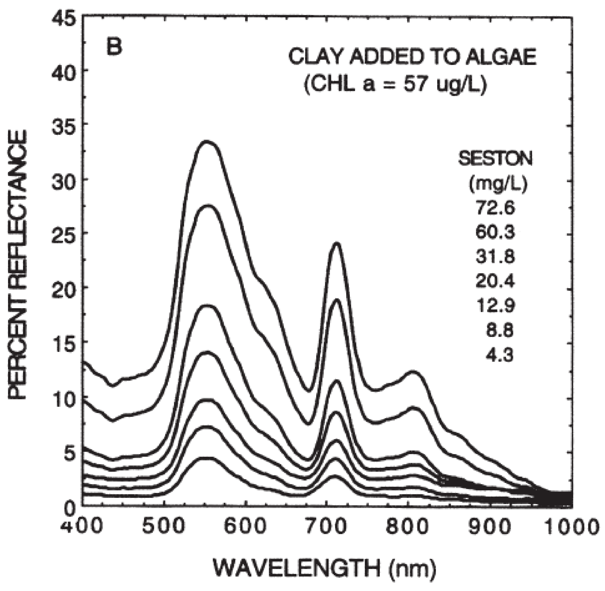
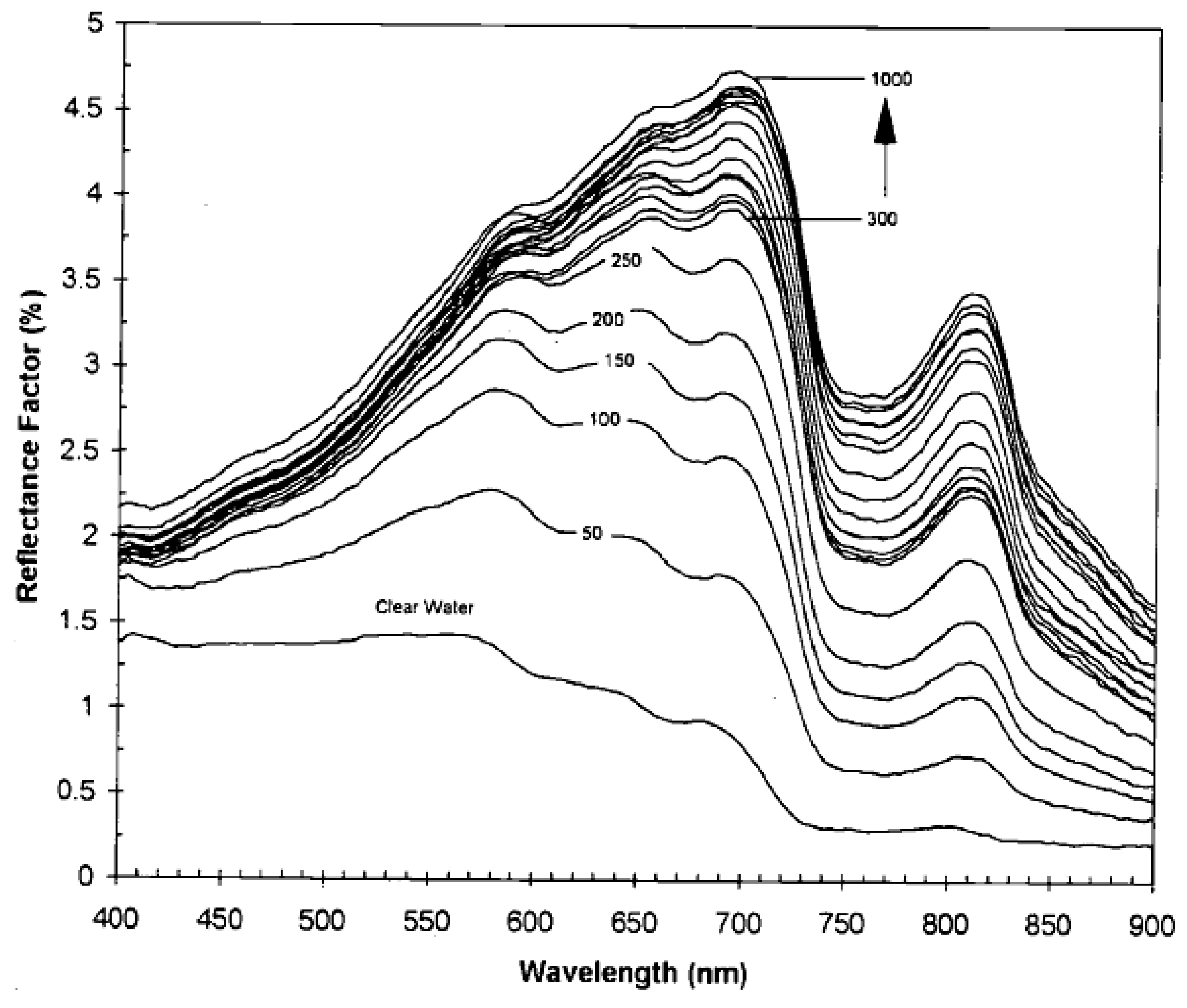
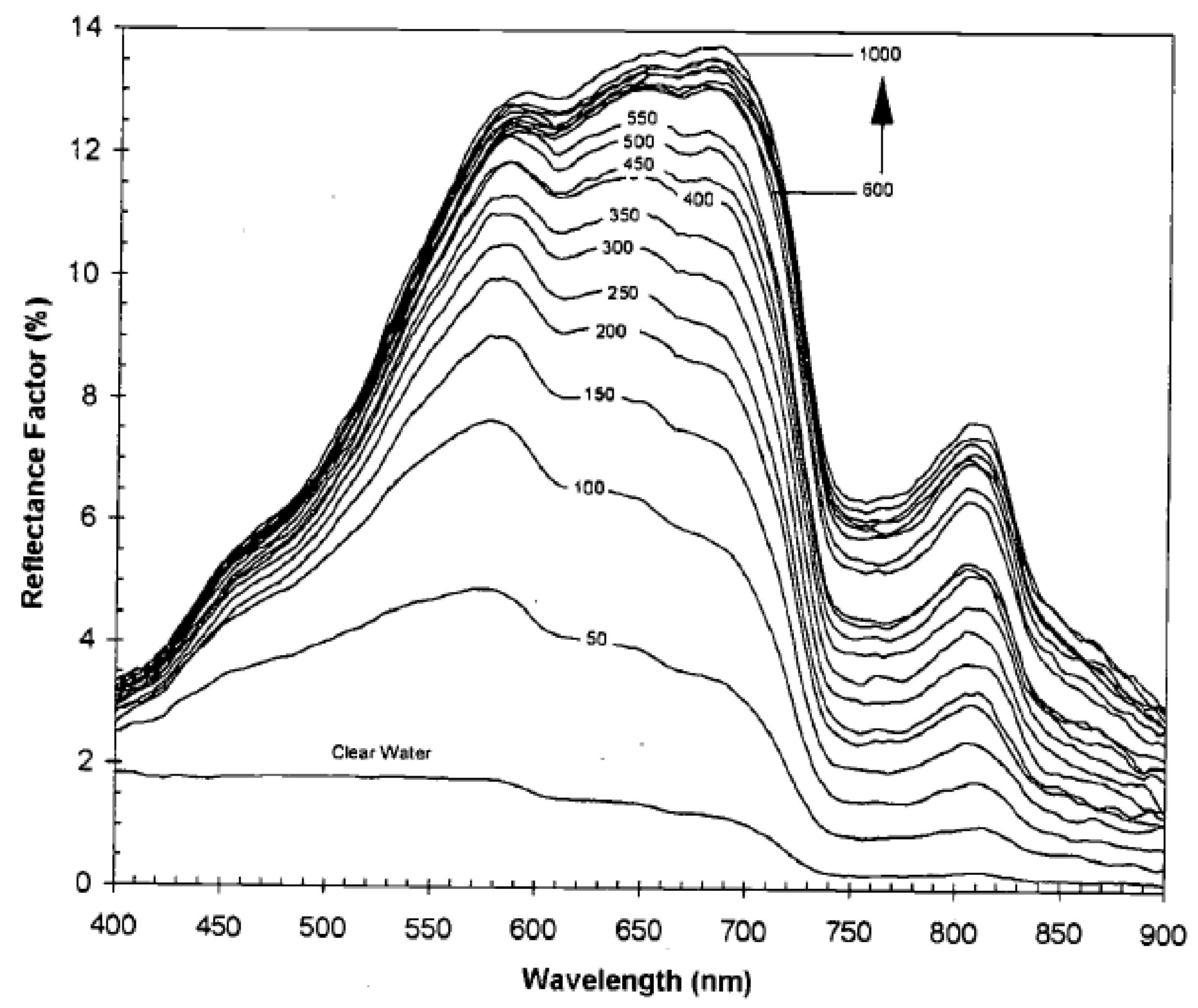
The presence of clay or dusty particles in water results in a specific spectrogram (Figure 3 and Figure 4) [18]. High reflectance in the range of 580–690 nm and reflectance near 810 nm will strongly distort the chlorophyll a spectrogram. The first range is characteristic for a specific type of suspension. In the case of lake bottom sediments that are composed of clay or dusty suspensions, they will have a similar spectrogram. The reflectance pattern around 810 nm is similar for clay and dusty suspensions and therefore, the reflectance around 810 nm can be used to estimate the suspension concentration.

Mathematical models using the reflectance R to determine the concentration of C_chl-a chlorophyll a in water are developed for a given type of surface water. These are the most abundant types of empirical models. Models such as GlobColour or Modis Aqua can be used globally or adapted to local reservoir conditions. They can take the form of polynomial dependence, as shown in the research of [19,20], dependence, as a form of the products or quotients of expressions [21,22], or a logarithmic form [23,24]. The estimation of model parameters can be carried out in different ways—using multiple linear recreation, support vector machine regression (SVR), or genetic algorithms. Examples of models used to determine the chlorophyll a content in the water are presented in

Table 1. Typical mathematical formulas to calculate chlorophyll a concentrations.

Formula	Source
Cchl-a=(23.09 ± 0.98) + (117.42 ± 2.49)·(R−1660–670 − R−1700–730)·R740–760 Cchl-a = −(16.2 ± 1.8) + (136.3 ± 3.2)·(R−1662–672 · R743–753)	(Gitelson et al., 2006) [21]
Cchl-a = (0.74·R681 + [(681 nm − 665 nm)/(681 nm − 620 nm)]·(R620 − R681) − R665	(Shen et al., 2010) [22]
log10(Cchl-a) = (0.32978 + 2.6465X + 1.9988X2 + 0.5708X3 + 3.033X4) X = log10(Max(R443nm, R486nm)/R551nm)	(Son et al., 2020) [23]
Cchl-a [mg/L] = 1.67 + 299 R438 − 33.1 R675 − 7217 R438R675 – 14022 R2438 − 973 R2675 + 373702 R2438R675 + 112440 R438R2675 − 3317051 R2438R2675 Cchl-a [mg/L] = 3.45 + 66.2 R438 − 100 R550 − 3.9 R675 + 5349 R438R550 − 16643 R550R675 − 12682 R438R675 + 3077 R2438 + 5209 R2550 + 15992 R2675	(Johan et al., 2018) [20]
log10(Cchl-a) = (0.366 − 3.067X + 1.930X2 + 6.049X3 − 1.532 X4) X = log10(Max(R443nm/R555nm, R490nm/R555nm, R510nm/R555nm))	GlobColour (Johnson et al., 2013) [25] (Diouf et al., 2018) [24]
log10(Cchl-a) = (0.6994 − 2.0384X + 0.4656RX2 + 0.4337X3) X = log10(Max(Rrs(443/555), Rrs(490=555)) Cchl-a = [mg/m3]	Modis-Aqua (Johnson et al., 2013) [24]

.

The models are characterized by a different precision of results. Johnson et al., 2013 [25], testing global models GlobColour or Modis Aqua, obtained low R² determination coefficients of 0.25–0.51; on the other hand, for local conditions, this indicator may reach up to the value 0.96, with an error for RMSE chlorophyll a content of 0.07 mg chl/m³, determined on the basis of a few data covering 5 days of composite images for the year 2014 [24].

Empirical models that are focused on determining the chlorophyll a concentration take into account the variability of the aquatic environment in terms of the content of other substances in a very limited way, which may affect the accuracy of the results obtained.

A possible solution to this problem in the case of inland waters may be the construction of seasonal models (used for imaging registered at specific seasons of the year) [26]. Another more widely used technique is the use of bioptic methods based on the modeling of light-water interaction, such as Hydrolight [27], or the newer 2SeaColor [28], adapted to water with high turbidity.

In the case of the second model, the determination indicator was equal 0.71, and model error RMSE was 6.23 mg chl/m³ [28]. Such models may include bottom reflectance [29,30], which is extremely important for shallow tanks, as pointed out by Hicks et al. 2013 [31].

In the works (Li et al., 2017, 2018) [32,33], a semi-analytical method for colored dissolved organic matter (CDOM) was presented. This method includes bottom effect and is accurate (RMSE = 0.17 mg chl/m³ and R² = 0.87); it also uses multispectral data.

The extremely promising result for turbid water research was the model developed by Gitelson et al. [21]. Finding three ranges of wavelengths guaranteeing the least error to estimate the chlorophyll a content enabled an accuracy of 7.8 mg chl a/m³ in the range of 1.2 to 236 mg chl a/m³, medium relative error 18.3%, with a high determination factor R² ≈ 0.96. The version of the model with two wave length ranges provided much worse results. Despite the high accuracy of in situ research for low concentrations (below 10 mg chl a/m³), there are relative errors reaching almost 100%.

Remote bathymetrical tests of shallow water, conducted by Lee et al. [34,35], yield the possibility of linking the effect of bottom reflectance and chlorophyll concentration. The developed model includes many different reflectances, including bottom reflectance and the absorption of radiation for various water components, such as phytoplankton pigments. However, the model is focused on the remote determination of depth. The number of model parameters is very large, making it troublesome to simultaneously determine the data for several wavelengths. Therefore, the absorption of radiation by phytoplankton is an input parameter for this model, not an output enabling the determination of chlorophyll concentration. In the case of oligotrophic sea waters, the computing models are simpler. Computational difficulties appear when many water components with spectrally different properties affect the calculation of the content of a given water component. This usually requires the use of the reflectances of many water components for many wave lengths. Particularly large complications appear in the case of shallow and turbid water.

The model of chlorophyll a content estimation in a reservoir used for drinking water intake was presented in this work. This application model is characterized by high accuracy, taking into account the bottom effect and interactions between chlorophyll and mineral or organic suspension.

2.2. Area of Study

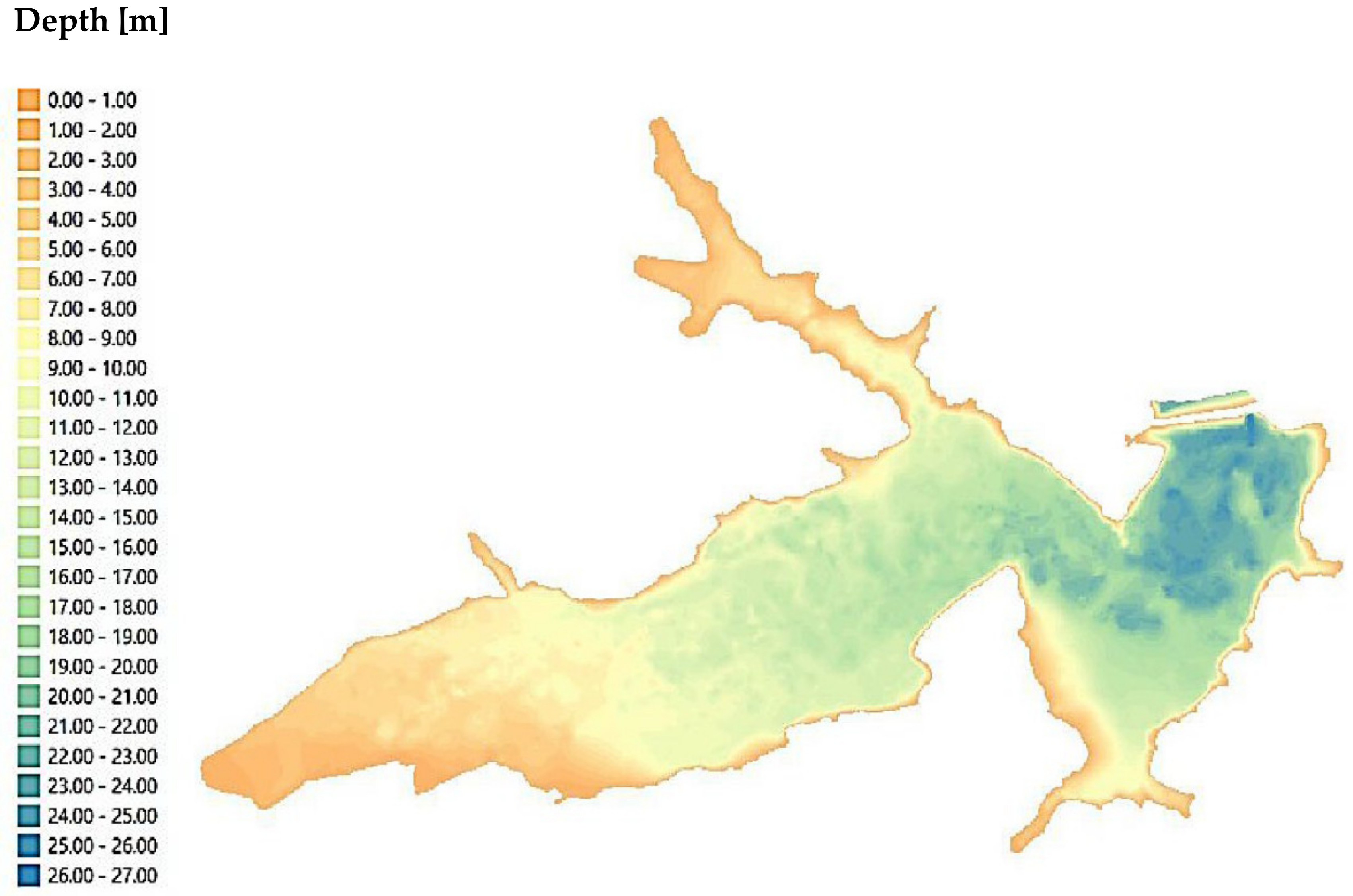
The research was carried out in the area of Lake Dobczyce, located in the Myślenice poviat, in the Lesser Poland voivodeship of Poland. It is a dam reservoir, constructed in 1986 by damming the Raba river with a 30 m high and 617 m long dam. The reservoir area is approximately 10.7 km², and its total capacity is 127 million m³. The reservoir serves as a source of drinking water. The lake water quality is determined by the quality of the Raba river, which varies due to anthropogenic activities and precipitation. These factors contribute to significant fluctuations in the concentrations of nutrients, mineral and organic suspensions, and other substances. The depth of the lake is just over twenty-six meters (Figure 5).

In the case of Dobczyce Lake, it is difficult to determine its range, especially in the western shallow region. This problem was solved by using information on the area elevation of the water surface and lidar altitude data (ALS), which, due to its high density, was subjected to resampling from the 5 × 5 m network using the MIN method, suggested by Śliwiński et al., 2022 [36], as the most suitable method for this type of task.

2.3. Data for a Remote Sensing Research

Images from Sentinel 2 (L1C product), registered from 13 April 2016 to 31 December 2021, were used for the teledetection quality modeling of water in Lake Dobczyce. The choice of specific images was determined by the dates of water quality tests in situ. A significant limitation in the number of images resulted from the rejection of images in which clouds or ice covered the lake.

The content of chlorophyll a and suspended solids (as turbidity) in the water was measured, in the period from 2016 to 2021, in the laboratory of the Waterworks of the City of Krakow, located at the water intake. The study covered the period from 2016 to 2021. Chlorophyll a was analyzed in acetone extracts using the monochromatic spectrophotometric method, with correction for pheopigment a [2,37]; absorbance was measured on a Hach DR 4000 U spectrophotometer, while turbidity was measured on a TL 2360 spectrophotometer, according to the standard methods [38].

2.4. Spectral Reflectance Curves

To compare the data recorded by Sentinel-2 satellites at different times, they were normalized to the conditions above the reference surface. The reference area was established as a fragment of the lakeside dam crest; it shows a low reflectance, and its properties are stable in time. The air composition over the reference surface was assumed to be the same as that over the lake surface. To correct lake surface reflectance obtained from satellite data, the special corrective parameter was introduced. It is the ratio of the reflectance registered on 13 April 2016 (13 April 2016, base date) in the reference field and the actual reflectance at a given day in the field. The normalized reflectance for the lake surface was the product of the corrective parameter and the reflectance of a given point on the lake surface at a given date. Such normalization is considered as an atmospheric correction. It made it possible to accommodate changes in air quality over the reference surface and the lake surface.

Spectral curves for the fragment of the dam crest are presented in Figure 6.

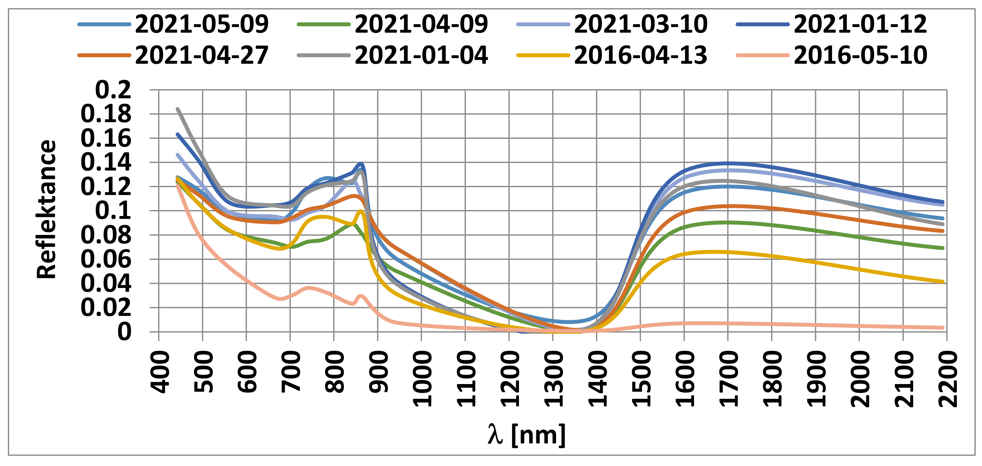
The base reflection curve for the fragment of the dam crest (reference area) is dated 13 April 2016 (Figure 6). Other spectral curves have a similar shape, but pass through points with different reflectance values, even though the properties of the dam crest surface have not changed; this was due to changes in the atmosphere composition over time.

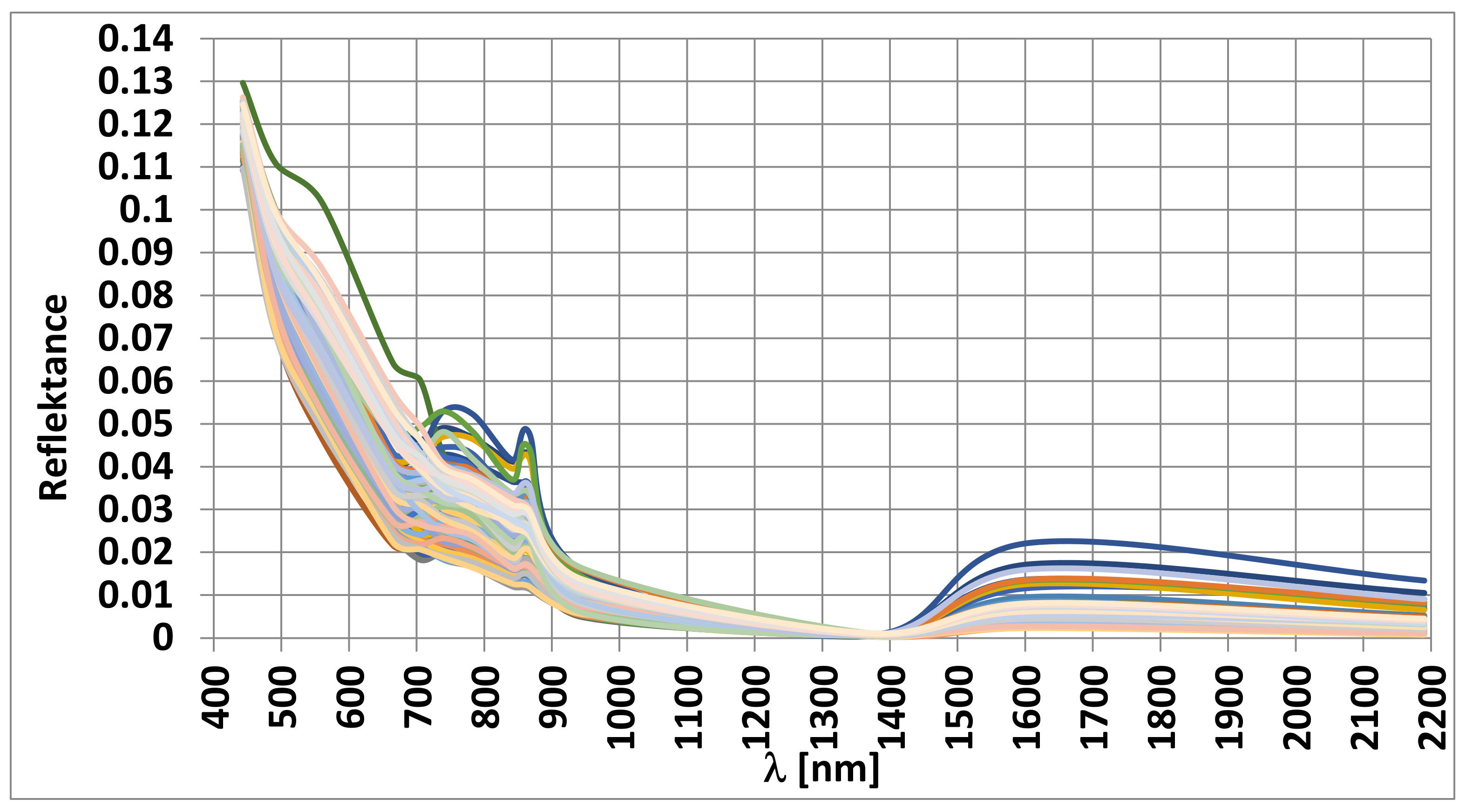
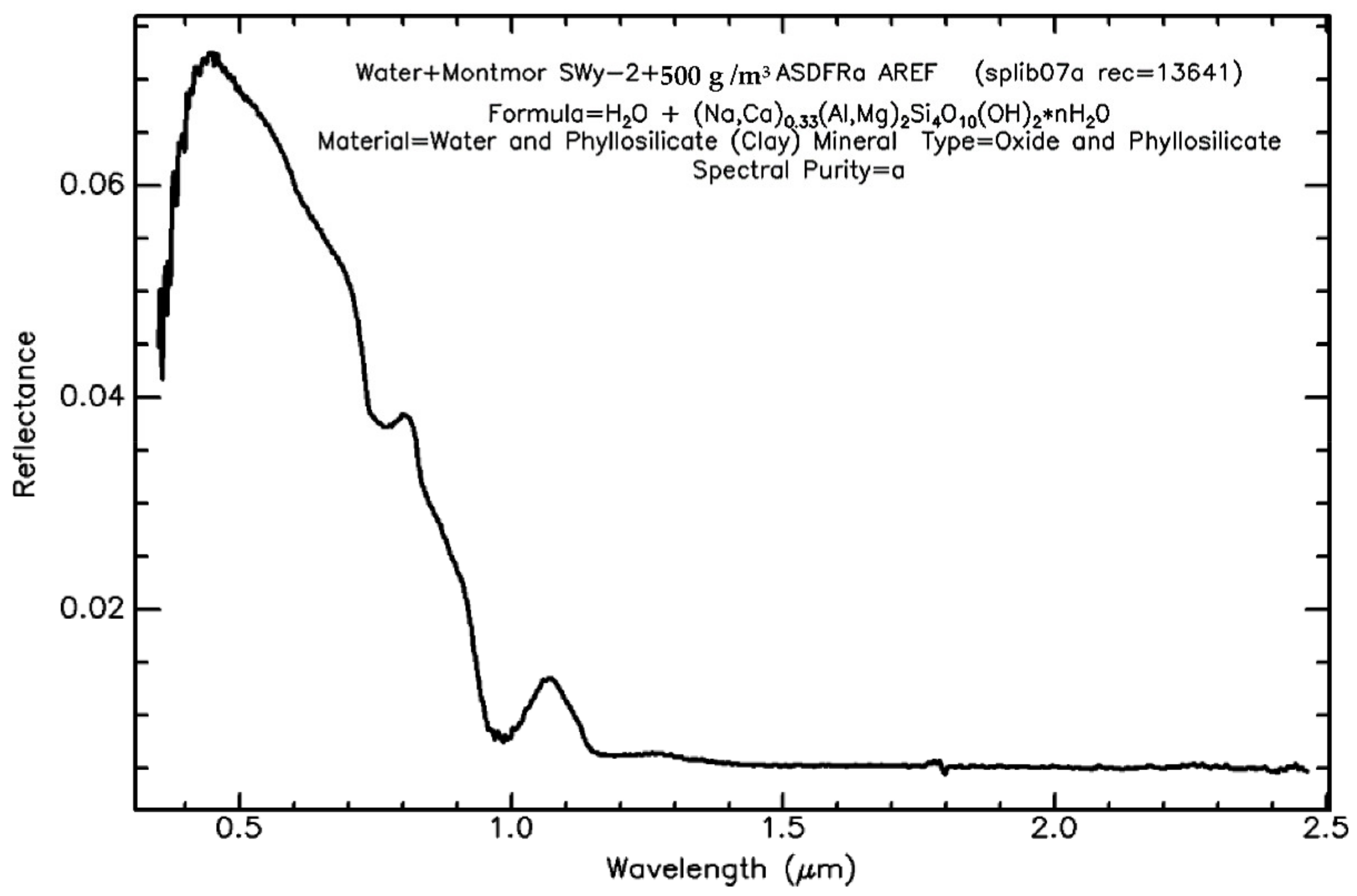
The specific course of the spectral curves for Lake Dobczyce (Figure 7) results from the combination (superposition) of partial spectral curves for the water surface, water column, and bottom of the reservoir. Backscattering in a blue band also results in high reflectance (Figure 7). It should be noted that even at a high concentration of, e.g., montmorillonite suspensions (500 g/m³), the spectral curve does not show strong local extremes for wavelengths over 440 nm (Figure 8). Such a concentration corresponds to a turbidity of 500 NTU, rarely found in surface waters (mostly after heavy rains). Starting from approximately 440 nm, the spectral curve drops down (Figure 8), as shown in the curves in Figure 7. At concentrations exceeding 500 g/m³, the maximum, corresponding to 440 nm, shifts towards longer wavelengths. The spectral curves may take completely different shapes than the ones shown in Figure 7 and Figure 8 for other types of the mineral suspensions.

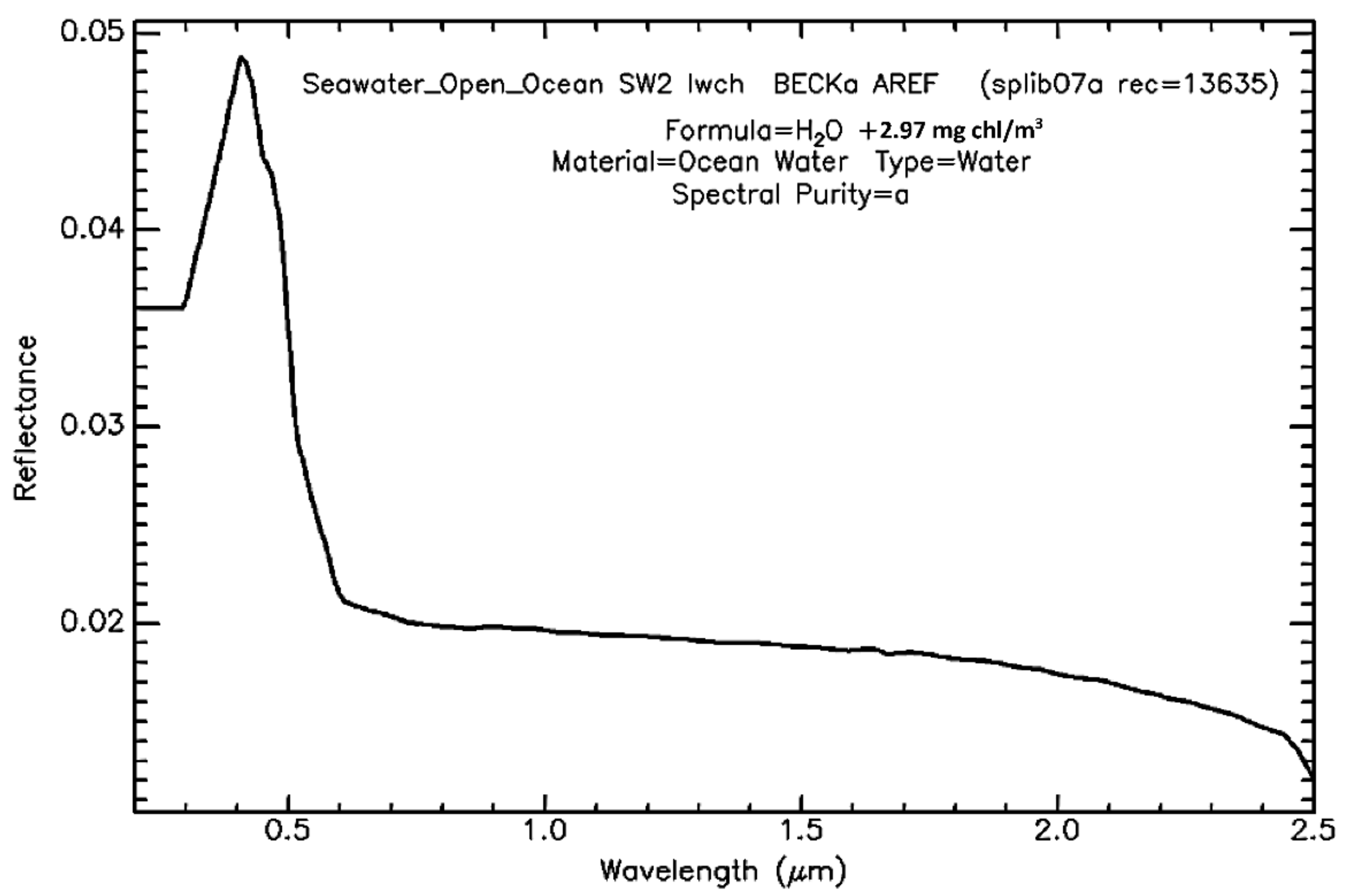
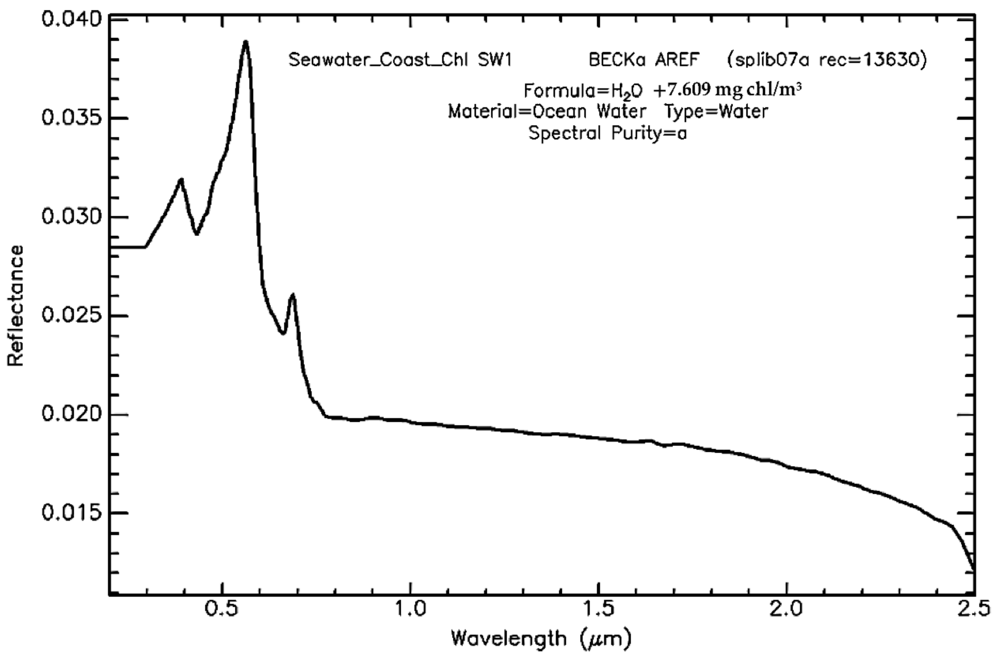
The spectral curves for the chlorophyll solution can also differ significantly. At low concentrations (2.97 mg chl/m³) (Figure 9), there are no strong local extremes on the spectral curve above 400 nm. Characteristic local extremes appear at higher concentrations (7.609 mg chl/m³) (Figure 10) and are similar to the curves in Figure 2. Therefore, it may be concluded that concentration of water components (chlorophyll, type of suspension) will have a decisive influence on the shape of the spectral curves.

2.5. Model

To compute concentrations of chlorophyll a (C_chl) from reflectance R obtained from satellite images for different wavelengths, a mathematical relationship has to be developed that meets the rules for logical concentration values for extremely high or low reflectance values. Empirical models, which are a linear combination of partial formulas, are risky to use because they cannot determine model parameters for all possible R values. The risk arises from a finite number of observational data, which usually does not include information on extreme values of R. Therefore, it may happen that C_chl calculated from the R values obtained from the new photos will be illogical, or even negative. Generally, extrapolation of such a model beyond the R values used to determine the model parameters yields highly ambiguous results; that is why models originating from the theory of dimensional analysis are considered to be safer. These types of models are usually the product of function modules at the appropriate power. They may also generate poor results outside of the R values used in the model estimation, but at least they guarantee that the results are positive.

The initial model was defined as:

$$C_{chl}={\alpha }_0{R}_{443}^{{\alpha }_1}{R}_{490}^{{\alpha }_2}{R}_{560}^{{\alpha }_3}{R}_{665}^{{\alpha }_4}{R}_{705}^{{\alpha }_5}{R}_{740}^{{\alpha }_6}{R}_{783}^{{\alpha }_7}{R}_{842}^{{\alpha }_8}{R}_{865}^{{\alpha }_9}{R}_{945}^{{\alpha }_{10}}{R}_{1375}^{{\alpha }_{11}}{R}_{1610}^{{\alpha }_{12}}{R}_{2190}^{{\alpha }_{13}}$$

(1)

where:

α₀ to α₁₃—model coefficients;

R_….—radiation reflectance for wavelengths: 443, 490, 560, 665, 705, 740, 783, 842, 865, 945, 1375, 1610, and 2190 nm, determined from the satellite data; and

C_chl—concentration of chlorophyll a [mg/m³].

The logarithmic Equation (1) leads to a linear relationship for the logarithms of reflectance R. The spectral curves of chlorophyll a (Figure 1) and the suspensions (Figure 2, Figure 3 and Figure 4) show that the reflectance for wavelengths over 865 nm and shorter than 490 nm will not provide significant information on the concentration of chlorophyll a. Therefore, the logarithmic form of Equation (1), after simplification, takes the form:

$$\begin{array}{l}\mathbf{ln}{C}_{chl}=a_0+a_1\mathbf{ln}{R}_{490}+a_2\mathbf{ln}{R}_{560}+a_3\mathbf{ln}{R}_{665}+a_4\mathbf{ln}{R}_{705}+\\ a_5\mathbf{ln}{R}_{740}+a_6\mathbf{ln}{R}_{783}+a_7\mathbf{ln}{R}_{842}+a_8\mathbf{ln}{R}_{865}\end{array}$$

(2)

where:

a₀ to a₈—model coefficients,

R_….—radiation reflectance for wavelengths: 490, 560, 665, 705, 740, 783, 842, and 865 nm, determined from the satellite data.

To make the model more general, additional components, like the squares of the reflectance log, were introduced:

$$\begin{array}{l}\mathbf{ln}{C}_{chl}=a_0+a_1\mathbf{ln}{R}_{490}+a_2\mathbf{ln}{R}_{650}+a_3\mathbf{ln}{R}_{665}+a_4\mathbf{ln}{R}_{705}+\\ a_5\mathbf{ln}{R}_{740}+a_6\mathbf{ln}{R}_{783}+a_7\mathbf{ln}{R}_{842}+a_8\mathbf{ln}{R}_{865}+a_9{\left(\mathbf{ln}{R}_{490}\right)}^2\\ a_{10}{\left(\mathbf{ln}{R}_{560}\right)}^2+a_{11}{\left(\mathbf{ln}{R}_{665}\right)}^2+a_{12}{\left(\mathbf{ln}{R}_{705}\right)}^2+a_{13}{\left(\mathbf{ln}{R}_{740}\right)}^2+\\ a_{14}{\left(\mathbf{ln}{R}_{783}\right)}^2+a_{15}{\left(\mathbf{ln}{R}_{842}\right)}^2+a_{16}{\left(\mathbf{ln}{R}_{865}\right)}^2\end{array}$$

(3)

The regression analysis of Equation (3) enabled the selection of such coefficients (from a₁ to a₁₆) that showed a probability lower than the significance coefficient 0.05 in the Student’s t-distribution (significance test of the equation coefficients). It was found that the most important coefficients are related to the wavelengths: 665, 705, 740, and 842 nm. These are the lengths approximately corresponding to the local minimum and maximum on the spectral curve of chlorophyll a (Figure 1 and Figure 2) and the local minimum and maximum on the spectral curve of the suspensions (Figure 2, Figure 3 and Figure 4). In the case of the Sentinel satellite, there were no 760 and 810 nm wavelength channels corresponding to the local minimum and maximum on the spectral curve of the suspensions (Figure 2, Figure 3 and Figure 4); hence, the 740 and 842 nm channels turned out to be statistically significant. Eventually, the model looked as follows:

$$\begin{array}{l}\mathbf{ln}{C}_{chl}=a_0+a_3\mathbf{ln}{R}_{665}+a_4\mathbf{ln}{R}_{705}+a_5\mathbf{ln}{R}_{740}+a_7\mathbf{ln}{R}_{842}+\\ a_{11}{\left(\mathbf{ln}{R}_{665}\right)}^2+a_{12}{\left(\mathbf{ln}{R}_{705}\right)}^2+a_{13}{\left(\mathbf{ln}{R}_{740}\right)}^2+a_{15}{\left(\mathbf{ln}{R}_{842}\right)}^2\end{array}$$

(4)

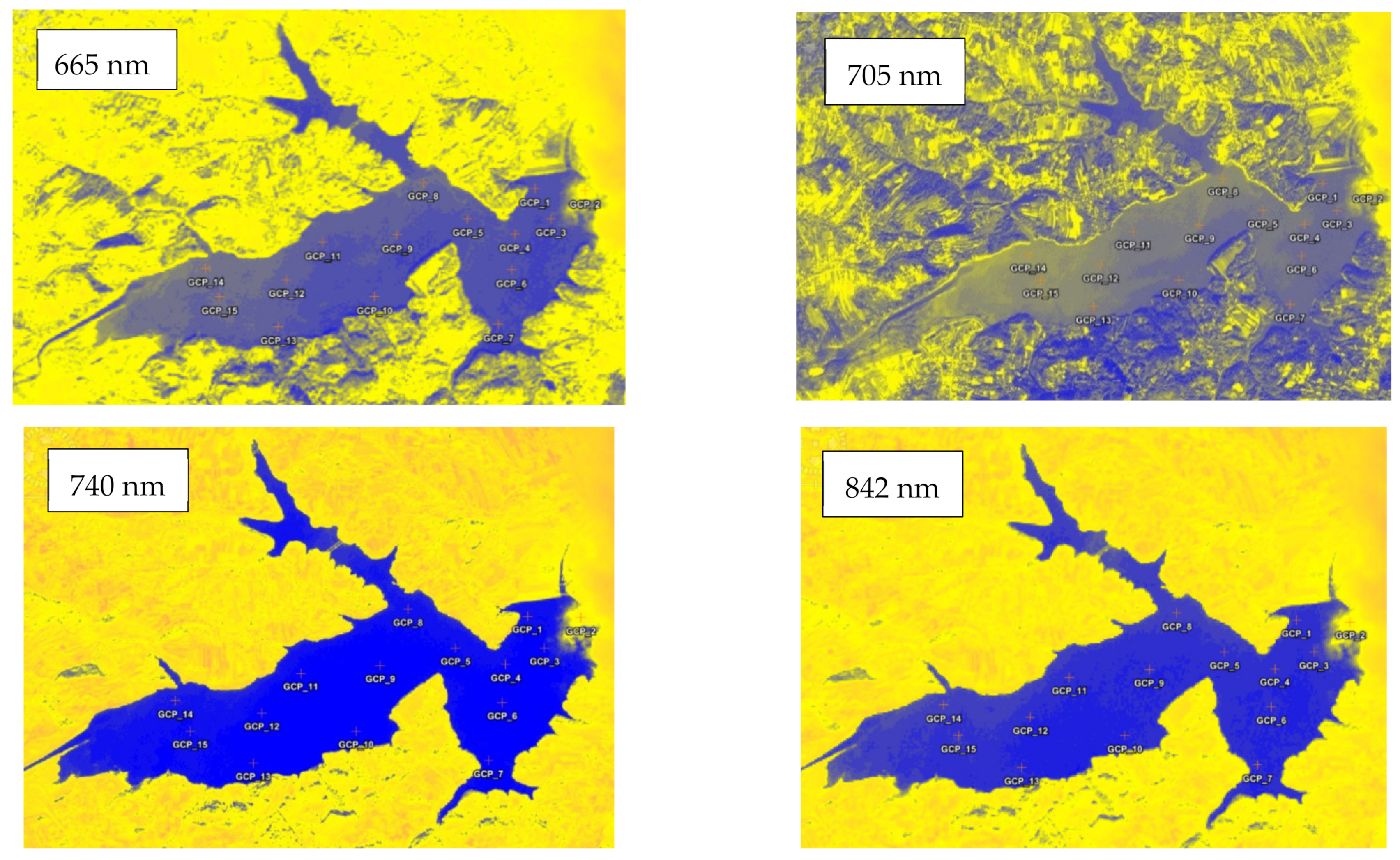
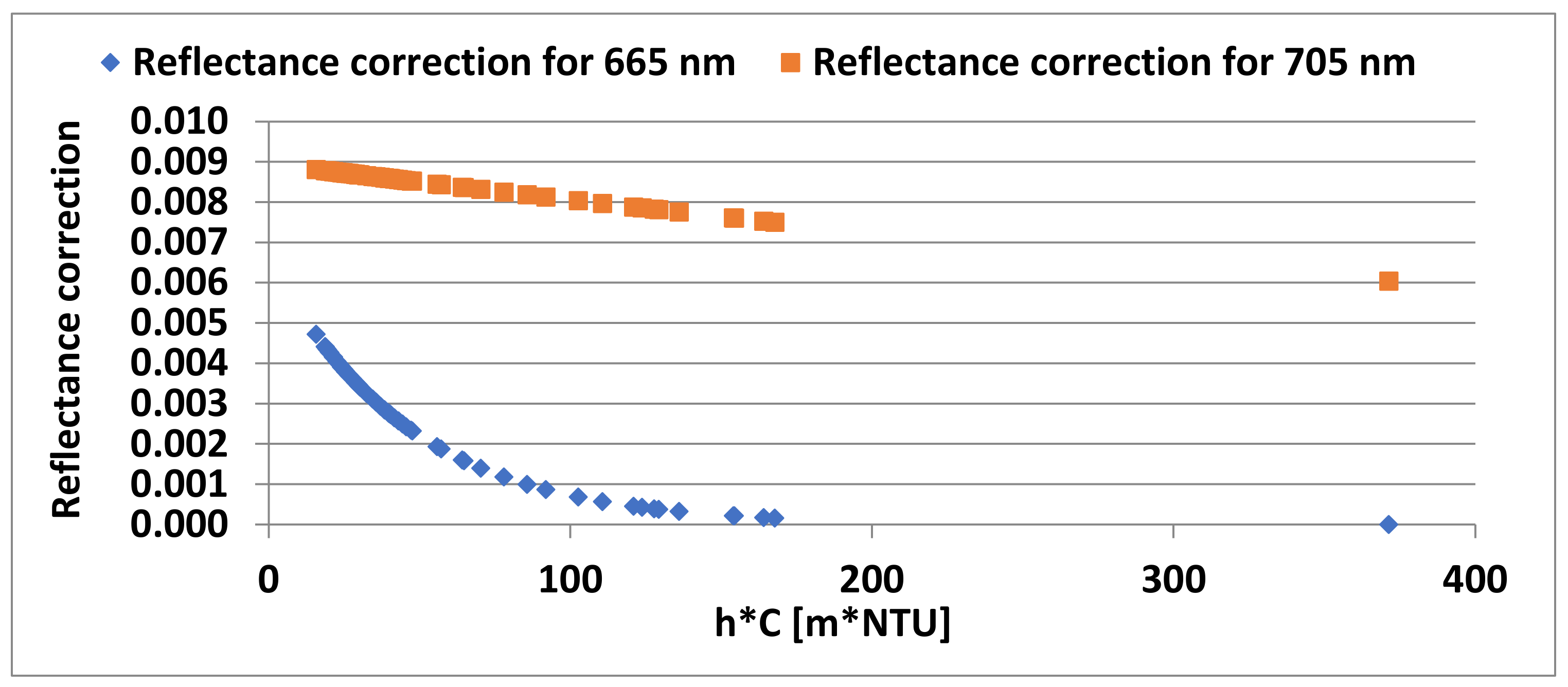
To eliminate the influence of the lake bottom reflectance, some reflectance corrections in Equation (4) were required. The effect of light reflection by the lake bottom in four light wavelengths is shown in Figure 11. However, just the reflectance corrections for 665 nm and 705 nm are sufficient for a good model accuracy. Of course, the reflectance for 740 nm and 842 nm may also be corrected, but their impact is negligible for the quality of the model (4). Generally, the shorter the wave, the stronger the bottom reflectance. Such observation is also confirmed by the spectral curves (Figure 7), which show that the shorter the wave, the higher the reflectance.

Following the Lambert–Beer law, absorbance (−ln(I/I₀)) of the medium for UV, Vis, and IR radiation is proportional to an optical path length l and a concentration of substance C. This means that a light intensity I in a water column decreases exponentially:

$$I=I_0·\mathbf{exp}\left(-k·C·l\right)$$

(5)

I₀—incident light intensity [W/m²];

k—absorption coefficient [m³/(g·m)];

C—concentration of a radiation absorber [g/m³];

l—optical path length [m].

Assuming that the lake bottom reflectance R_b is approximately proportional to the intensity of the radiation reaching the depth of l = h, the reflectance over a water surface, recorded by a photosensitive sensor, would be described by the relationship:

$$R_b=\frac{{\alpha }_b·I_0·\mathbf{exp}\left(-k·C·2h\right)}{I_0}={\alpha }_b·\mathbf{exp}\left(-k·C·2h\right)$$

(6)

α_b—coefficient of the radiation reflectance through the bottom;

C—concentration of all substances (e.g., chlorophyll a, mineral suspensions, organic suspensions, water) responsible for absorption of radiation [g/m³], i.e., water turbidity [NTU];

h—depth (actual length of an optical path, when shooting close to the zenith, is approximately equal to the depth h) [m].

The number 2 in Formula (6) means that radiation passes twice through the water layer.

The reflectance R, recorded by the satellite, is approximately equal to the sum of the four principal reflectances:

$$\begin{array}{l}R=\frac{{\alpha }_s{I}_0+I_{chl}+I_m+{\alpha }_b(I_0-{\alpha }_s{I}_0)\mathbf{exp}\left(-k·C·2h\right)}{I_0}=\\ {\alpha }_s+\frac{I_{chl}}{I_0}+\frac{I_m}{I_0}+{\alpha }_b(1-{\alpha }_s)\mathbf{exp}\left(-k·C·2h\right)=\\ {\alpha }_s+R_{chl}+R_m+{\alpha }_b(1-{\alpha }_s)\mathbf{exp}\left(-k·C·2h\right)\end{array}$$

(7)

${\alpha }_s$—coefficient of the radiation reflectance for the water surface (water surface reflectance);

$R_{chl}$—reflectance related to chlorophyll a in water, as the total effect of radiation;

$I_{chl}$—reflected at different water depths;

$R_m$—reflectance related to the substances, other than chlorophyll a, in water, as the total effect of radiation $I_m$ reflected at different water depths;

${\alpha }_b(1-{\alpha }_s)\mathbf{exp}\left(-k·C·2h\right)$—reflectance of the lake bottom R_b.

Intensity of radiation $I_{chl}$, $I_m$ reflected from water at different depths is defined as the depth integration from the derivative of the radiation intensity at different depths, with respect to the depth defined by (5); intensity $I_0$ must be reduced by the intensity of the radiation reflected from the water surface ${\alpha }_s{I}_0$. Therefore:

$$\begin{array}{l}{I}_{chl}=-{\displaystyle \underset{0}{\overset{h}{\int }}\frac{d\left({\alpha }_{chl}{C}_{chl}(I_0-{\alpha }_s{I}_0)\mathbf{exp}\left(-k·C·2l\right)\right)}{dl}dl=}\\ {\alpha }_{chl}{C}_{chl}(I_0-{\alpha }_s{I}_0)\left(1-\mathbf{exp}\left(-k·C·2h\right)\right)\end{array}$$

(8)

$$\begin{array}{l}{I}_m=-{\displaystyle \underset{0}{\overset{h}{\int }}\frac{d\left({\alpha }_m{C}_m(I_0-{\alpha }_s{I}_0)\mathbf{exp}\left(-k·C·2l\right)\right)}{dl}dl=}\\ {\alpha }_m{C}_m(I_0-{\alpha }_s{I}_0)\left(1-\mathbf{exp}\left(-k·C·2h\right)\right)\end{array}$$

(9)

C_chl—concentration of chlorophyll a [mg/m³];

α_chl—coefficient of the radiation reflectance for chlorophyll a [m³/mg];

C_m—concentration of non-chlorophyll a substances in water responsible for light reflection [g/m³];

α_m—coefficient of the radiation reflectance for substances other than chlorophyll a [m³/g].

If h and/or C are sufficiently high, then $\mathbf{exp}\left(-k·C·2h\right)<<1$ and:

$$I_{chl}\approx {\alpha }_{chl}{C}_{chl}(I_0-{\alpha }_s{I}_0)\hspace{1em}\Rightarrow \hspace{1em}{R}_{chl}\approx {\alpha }_{chl}{C}_{chl}(1-{\alpha }_s)$$

(10)

$$I_m\approx {\alpha }_m{C}_m(I_0-{\alpha }_s{I}_0)\hspace{1em}\Rightarrow \hspace{1em}{R}_m\approx {\alpha }_m{C}_m(1-{\alpha }_s)$$

(11)

In model (4), the R… reflectance for different wavelengths is the computational reflectance R_calc, which are formally sums $R_{chl,\hspace{0.33em}\dots }+R_{m,\hspace{0.33em}\dots }$ for different wavelengths. Therefore, each reflectance in model (4) should be corrected and replaced with the computational reflectance for different wavelengths:

$$\begin{array}{l}{R}_{\dots }\leftarrow R_{calc,\hspace{0.33em}\dots }=R_{chl,\hspace{0.33em}\dots }+R_{m,\hspace{0.33em}\dots }=\\ R_{\dots }-{\alpha }_{s,\hspace{0.33em}\dots }-{\alpha }_{b,\hspace{0.33em}\dots }(1-{\alpha }_{s,\hspace{0.33em}\dots })\mathbf{exp}\left(-k_{\dots }·C·2h\right)\end{array}$$

(12)

⃞_…—the index dots refer to different wavelengths;

R_….—radiation reflectance for different wavelengths determined from satellite;

$R_{calc,\hspace{0.33em}\dots }$—computational reflectance for different wavelengths.

The coefficient ${\alpha }_s$ (or reflectance) for different wavelengths is small if compared to other reflectance, and therefore should be neglected, so:

$$\begin{array}{l}{R}_{\dots }\leftarrow R_{calc,\hspace{0.33em}\dots }=R_{chl,\hspace{0.33em}\dots }+R_{m,\hspace{0.33em}\dots }=\\ R_{\dots }-{\alpha }_{b,\hspace{0.33em}\dots }\mathbf{exp}\left(-k_{\dots }·C·2h\right)\end{array}$$

(13)

A reflectance correction (13) in Equation (4) gives the equation describing the concentration of chlorophyll a as:

$$\begin{array}{cc}\hfill & C_{chl}=\mathbf{exp}\left[a_0+a_3\mathbf{ln}{\left(R_{665}-{\alpha }_{b,665}\mathbf{exp}\left(-k_{665}·C·2h\right)\right)}^{}\right.+\hfill \\ \hfill & a_4\mathbf{ln}{\left(R_{705}-{\alpha }_{b,705}\mathbf{exp}\left(-k_{705}·C·2h\right)\right)}^{}+\hfill \\ \hfill & a_5\mathbf{ln}{R}_{740}+a_7\mathbf{ln}{R}_{842}+\hfill \\ \hfill & a_{11}{\left(\mathbf{ln}\left(R_{665}-{\alpha }_{b,665}\mathbf{exp}\left(-k_{665}·C·2h\right)\right)\right)}^2+\hfill \\ \hfill & a_{12}{\left(\mathbf{ln}\left(R_{705}-{\alpha }_{b,705}\mathbf{exp}\left(-k_{705}·C·2h\right)\right)\right)}^2+\hfill \\ \hfill & \left.a_{13}{\left(\mathbf{ln}{R}_{740}\right)}^2+a_{15}{\left(\mathbf{ln}{R}_{842}\right)}^2\right]\hfill \end{array}$$

(14)

$C_{chl}$—chlorophyll a concentration [mg/m³];

$\mathbf{exp}(a_0)$—model’s coefficient [mg/m³].

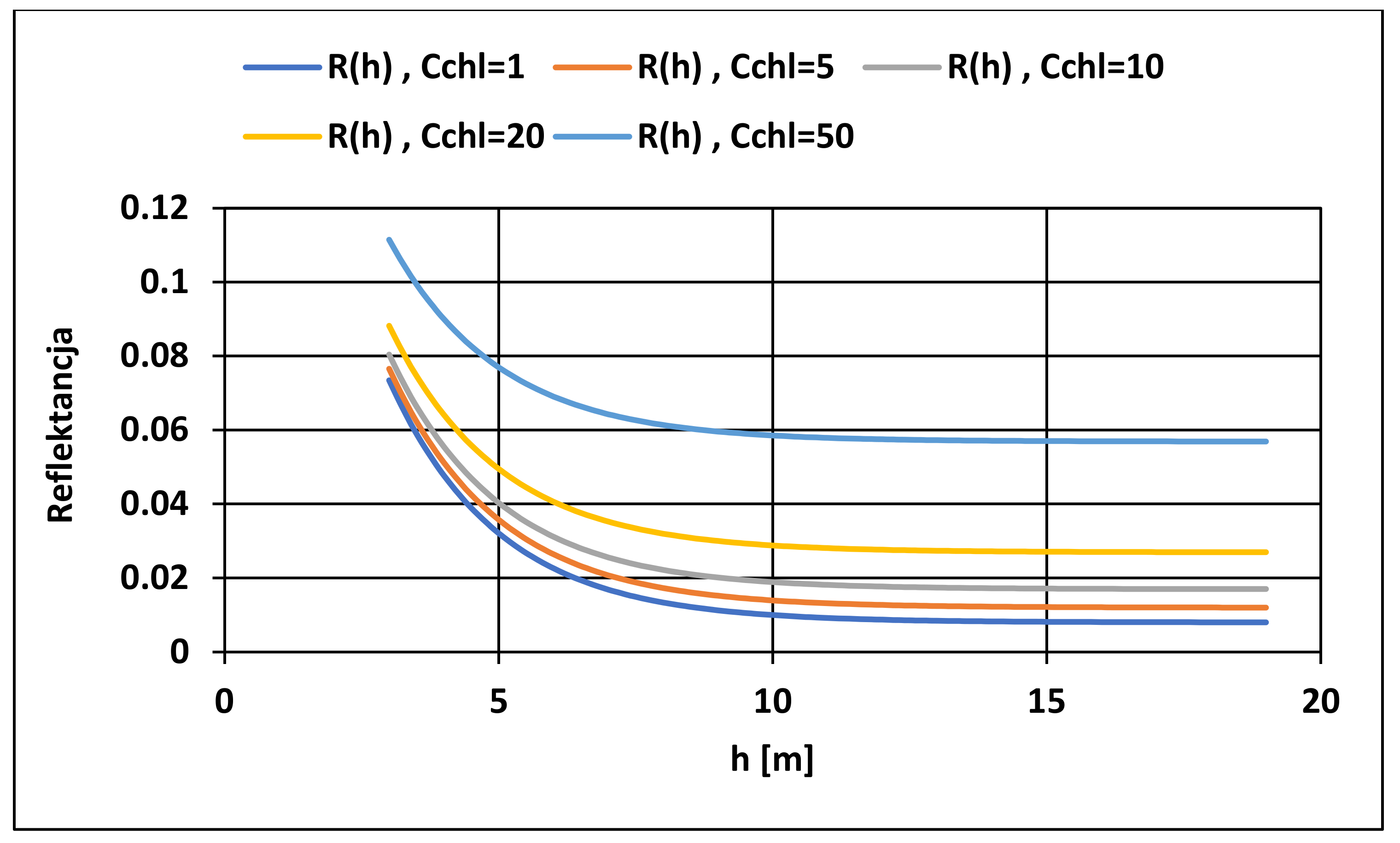
Assume the following parameter values for Equations (7)–(9) relating to one wavelength: ${\alpha }_s$ = 0.002, ${\alpha }_m$ = 0.001, ${\alpha }_b$ = 0.3, ${\alpha }_{chl}$ = 0.001, $k$ = 0.05 (NTU·m)⁻¹, C_m = $C\approx$ 5 NTU (in practice, water turbidity is assumed as C) and $C_{chl}$ = {1, 5, 10, 20, 50} mg/m³. From the Equations (7)–(9), the reflectance R can be determined, as a function of the depth h (Figure 12). Knowing R and the parameters of Equations (7)–(9), the concentration of chlorophyll a $C_{chl}$ can be again determined. These would be horizontal lines of constant values $C_{chl}$ = {1, 5, 10, 20, 50} mg/m³ for all depths h. In order to check the quality of the model (14), we write it for a single wavelength:

$$\begin{array}{l}{C}_{chl}=\mathbf{exp}\left[a_0+a_3\mathbf{ln}{\left(R-{\alpha }_b^{\ast }\mathbf{exp}\left(-k^{\ast }·C·2h\right)\right)}^{}\right.+\\ \left.a_{11}{\left(\mathbf{ln}\left(R-{\alpha }_b^{\ast }\mathbf{exp}\left(-k^{\ast }·C·2h\right)\right)\right)}^2\right]\end{array}$$

(15)

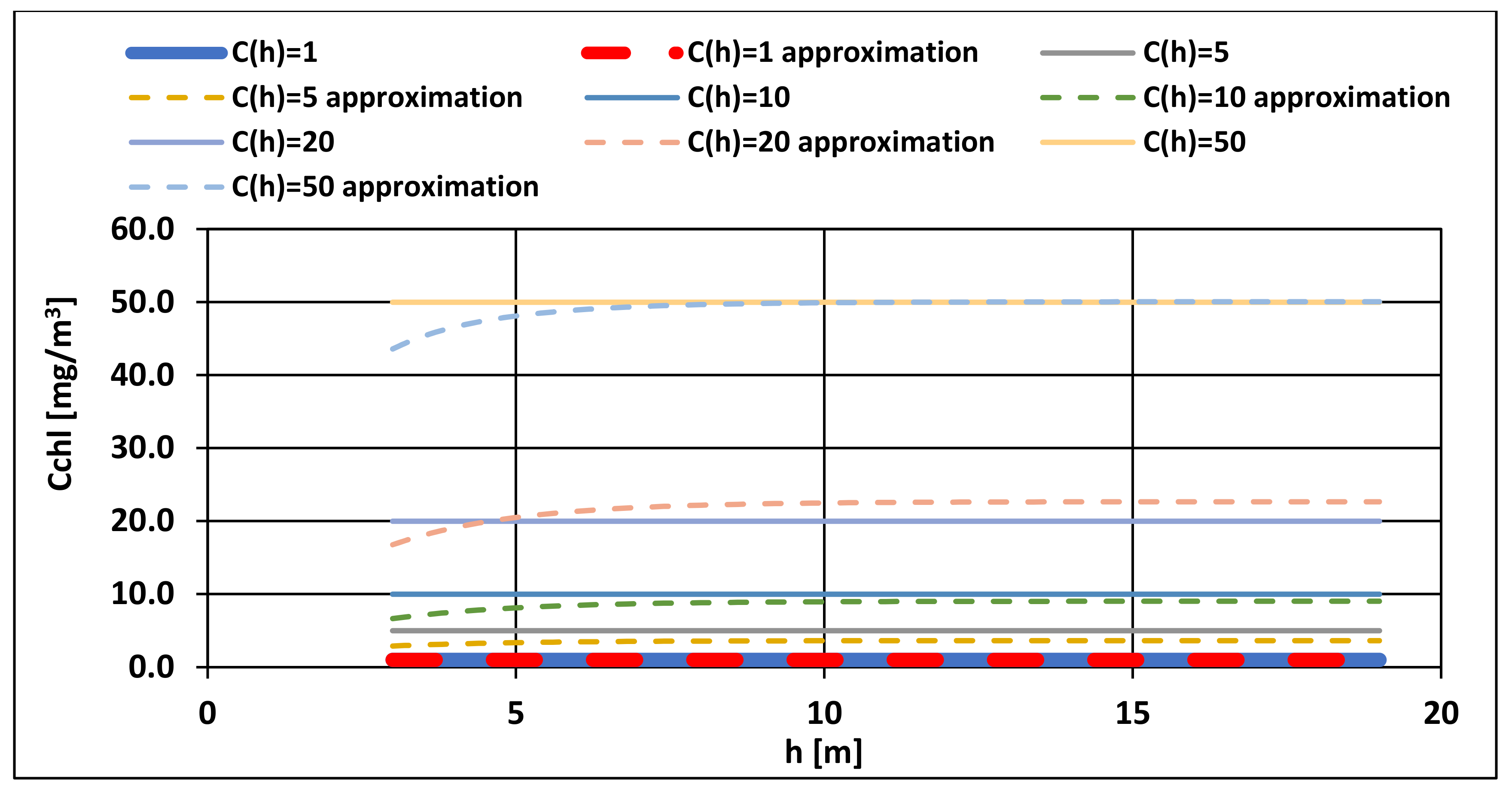
The parameters of model (15) were determined on the basis of changes in reflectance R as a function of h, determined from Equations (7)–(9). The following parameters were obtained: $a_0$ = −0.994654, $a_3$ = −3.91129, ${\alpha }_b^{\ast }$ = 0.293404, $k^{\ast }$ = 0.04999945 (NTU·m)⁻¹, $a_{11}$ = −0.767181. Parameters: ${\alpha }_b^{\ast }$ and $k^{\ast }$ are almost equal to ${\alpha }_b$ = 0.3, $k$ = 0.05 (NTU·m)⁻¹ used in Equations (7)–(9). Formally, ${\alpha }_b^{\ast }$ should be equal to ${\alpha }_s+{\alpha }_b^{}\left(1-{\alpha }_s\right)$ = 0.002 + 0.3·(1 − 0.002) = 0.3014, as in Equation (12). The compliance of the parameters ${\alpha }_b^{\ast }$ and $k^{\ast }$ with the parameters ${\alpha }_b$ and $k$ confirms that a correction (13) for the bottom reflectance in the models (14) and (15) was needed. Model (15) is less accurate for shallow depths and higher concentrations of chlorophyll a C_chl (Figure 13), along with model (14).

It would be difficult to use a combination of Equations (7)–(9) to calculate chlorophyll a concentrations on the basis of the reflectance recorded by a satellite; such reflectance is a combination of both a chlorophyll a reflectance and the reflectance of other substances present in the water. Such calculations were performed for the wavelengths of 665 nm and 705 nm. However, accurate parameters of models (7)–(9) for one wavelength and known turbidity could not be found. Therefore, model (14) has been proposed as the one that that includes the reflectance for different wavelengths.

3. Results

3.1. Model Parameters for Chlorophyll a

Based on the measurements of the concentration of chlorophyll a C_chl, turbidity C, lake depth h, and the reflectance R… for wavelengths: 665, 705, 740, and 842 nm, the model parameters were determined (14). Due to the large number of parameters:

$$a_0\hspace{0.33em},\hspace{0.33em}{a}_3\hspace{0.33em},\hspace{0.33em}{\alpha }_{b,\hspace{0.33em}665}\hspace{0.33em},\hspace{0.33em}{k}_{665}^{}\hspace{0.33em},\hspace{0.33em}{a}_4\hspace{0.33em},\hspace{0.33em}{\alpha }_{b,\hspace{0.33em}705}\hspace{0.33em},\hspace{0.33em}{k}_{705}^{}\hspace{0.33em},\hspace{0.33em}{a}_5\hspace{0.33em},\hspace{0.33em}{a}_7\hspace{0.33em},\hspace{0.33em}{a}_{11}\hspace{0.33em},\hspace{0.33em}{a}_{12}\hspace{0.33em},\hspace{0.33em}{a}_{13}\hspace{0.33em},\hspace{0.33em}{a}_{15}$$

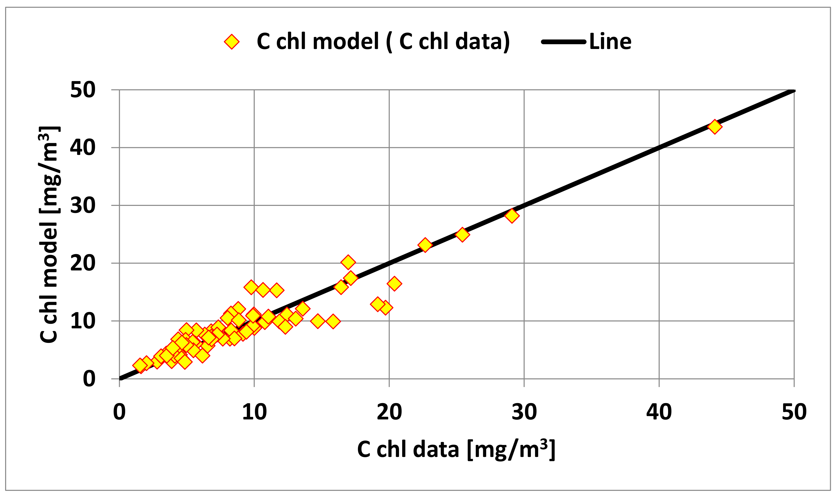
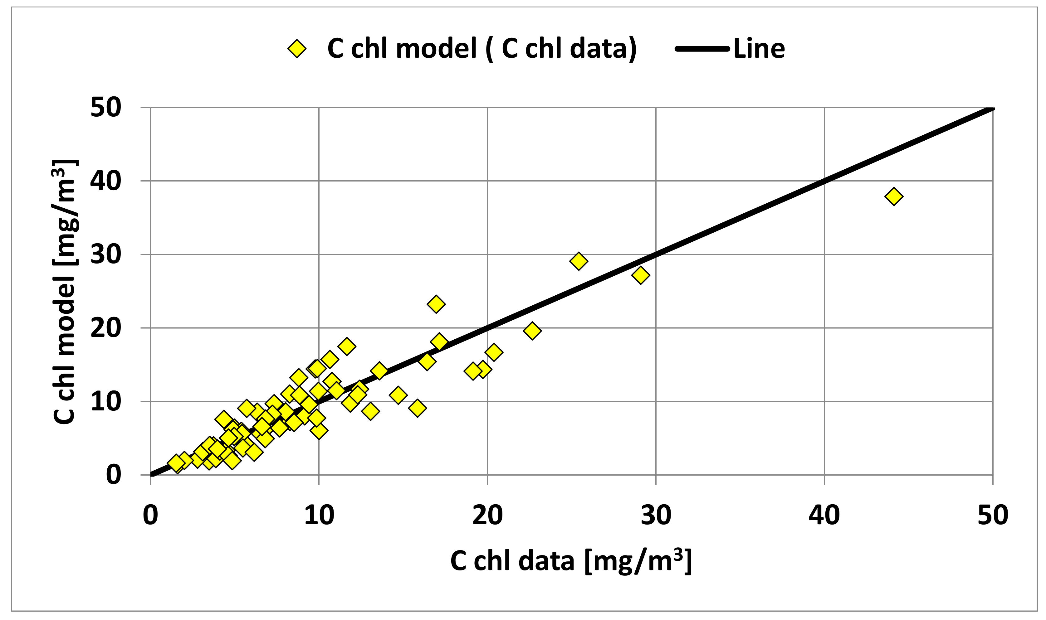
the two-stage procedure was introduced. At first, a preliminary estimate of the parameters: $a_0\hspace{0.33em},\hspace{0.33em}{a}_3\hspace{0.33em},\hspace{0.33em}{a}_4\hspace{0.33em},\hspace{0.33em}{a}_5\hspace{0.33em},\hspace{0.33em}{a}_7\hspace{0.33em},\hspace{0.33em}{a}_{11}\hspace{0.33em},\hspace{0.33em}{a}_{12}\hspace{0.33em},\hspace{0.33em}{a}_{13}\hspace{0.33em},\hspace{0.33em}{a}_{15}$ was produced for the logarithm of r (4) using the least square method, i.e., minimizing the sum of squares of deviations between the logarithm of the measured chlorophyll concentration C_chl and the logarithm of the concentration calculated from model (4). Then, other model parameters were found, assuming the parameter values previously determined for model (4) for the calculations. All parameters were determined by minimizing the sum of squared deviations between the measured C_chl concentration and the one calculated from model (14); the correlation coefficient was 0.944. The values of the model parameters (14) are summarized in

Table 2. Model parameters (14).

Parameter	Value at Known Turbidity	Value at Turbidity Calculated from Model (17)	Units
1	2	3	4
$a_0$	−32.25907512	−75.68466110	ln(mg/m3)
$a_3$	−43.55040094	−72.72855795	–
${\alpha }_{b,\hspace{0.33em}665}$	0.015293030	0.006693771	–
$k_{665}$	0.007665104	0.011140396	(NTU·m)−1
$a_4$	42.36776151	62.29811979	–
${\alpha }_{b,\hspace{0.33em}705}$	0.010635655	0.008960131	–
$k_{705}$	0.003498578	0.000530822	(NTU·m)−1
$a_5$	−23.86732103	−47.45269805	–
$a_7$	4.731529537	9.465054057	–
$a_{11}$	−5.149196218	−9.056892001	–
$a_{12}$	4.533167105	6.641324249	–
$a_{13}$	−2.345421643	−5.388690882	–
$a_{15}$	0.193746731	0.802524849	–

, col. 2. The model fit is shown in Figure 14. If turbidity was calculated from model (17), the parameters of model (14) would have been provided, as shown in Table 2, col. 3. The correlation coefficient was 0.925. The fit of model (14), while using model (17), is shown in Figure 15. In both cases, the model’s fit to the measurements was good. If there is no detailed data on turbidity and the parameter shows little variability, the average value of turbidity can be used in the calculations.

3.2. Maps of Chlorophyll a Concentrations for Lake Dobczyce

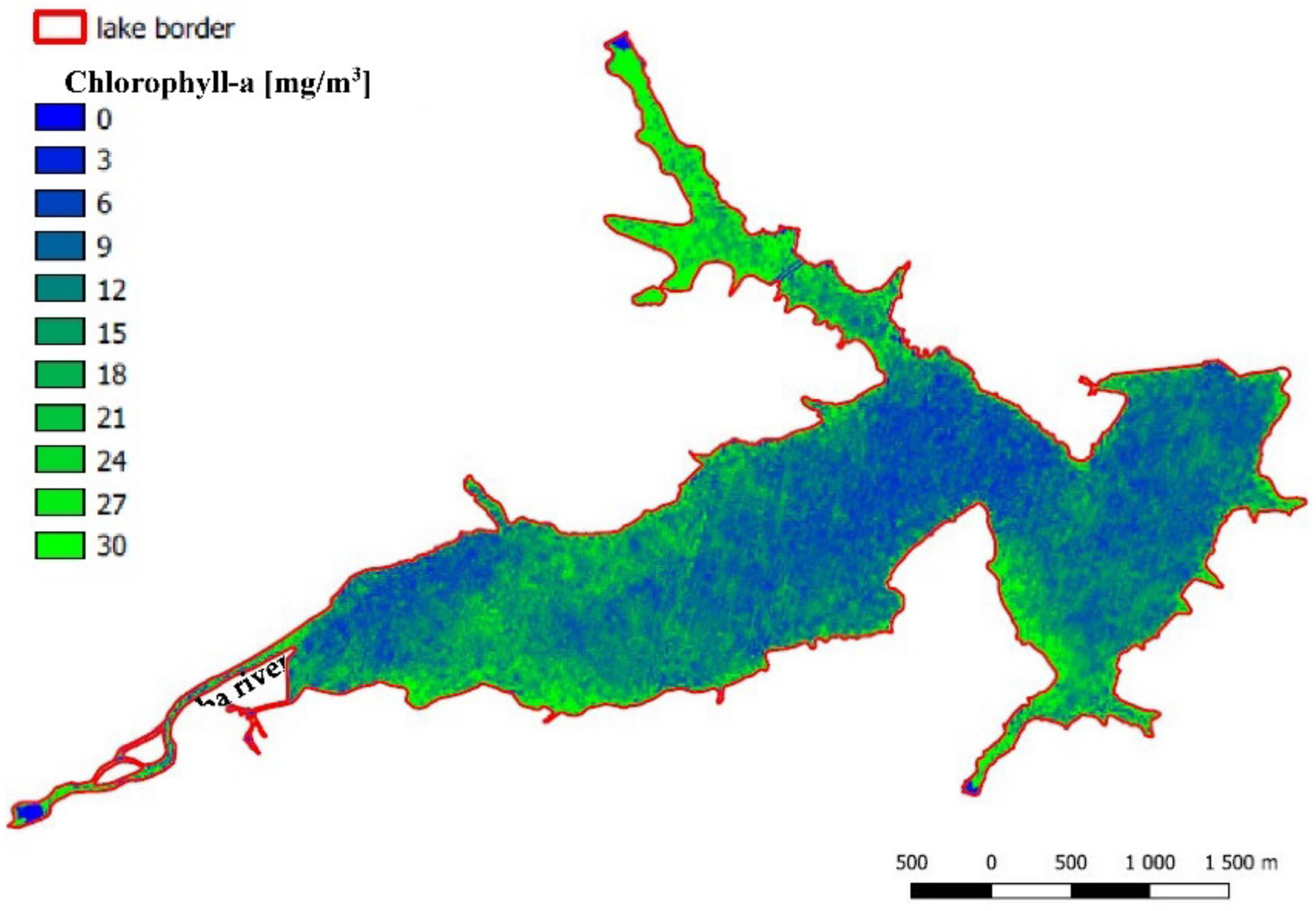
The map of chlorophyll a concentrations (Figure 16) was developed from satellite images using models (14) and (17). Long retention times observed in Lake Dobczyce (average 157 days), contribute to the algae growth and high chlorophyll a concentrations; higher concentrations are noted in the middle of the lake. In this region, towards the dam, low flow velocities are also observed (Figure 17); therefore, concentrations slightly decrease due to sedimentation of the suspended solids and algae. There are stagnant zones at the northern and southern banks of the lake, where flow velocities are very low (Figure 17). Such conditions promote algae growth, and the observed concentration of chlorophyll a is high. Moreover, in the lake branches, where a water exchange is low and the retention times exceed the average one, high concentrations of chlorophyll a are observed (Figure 16).

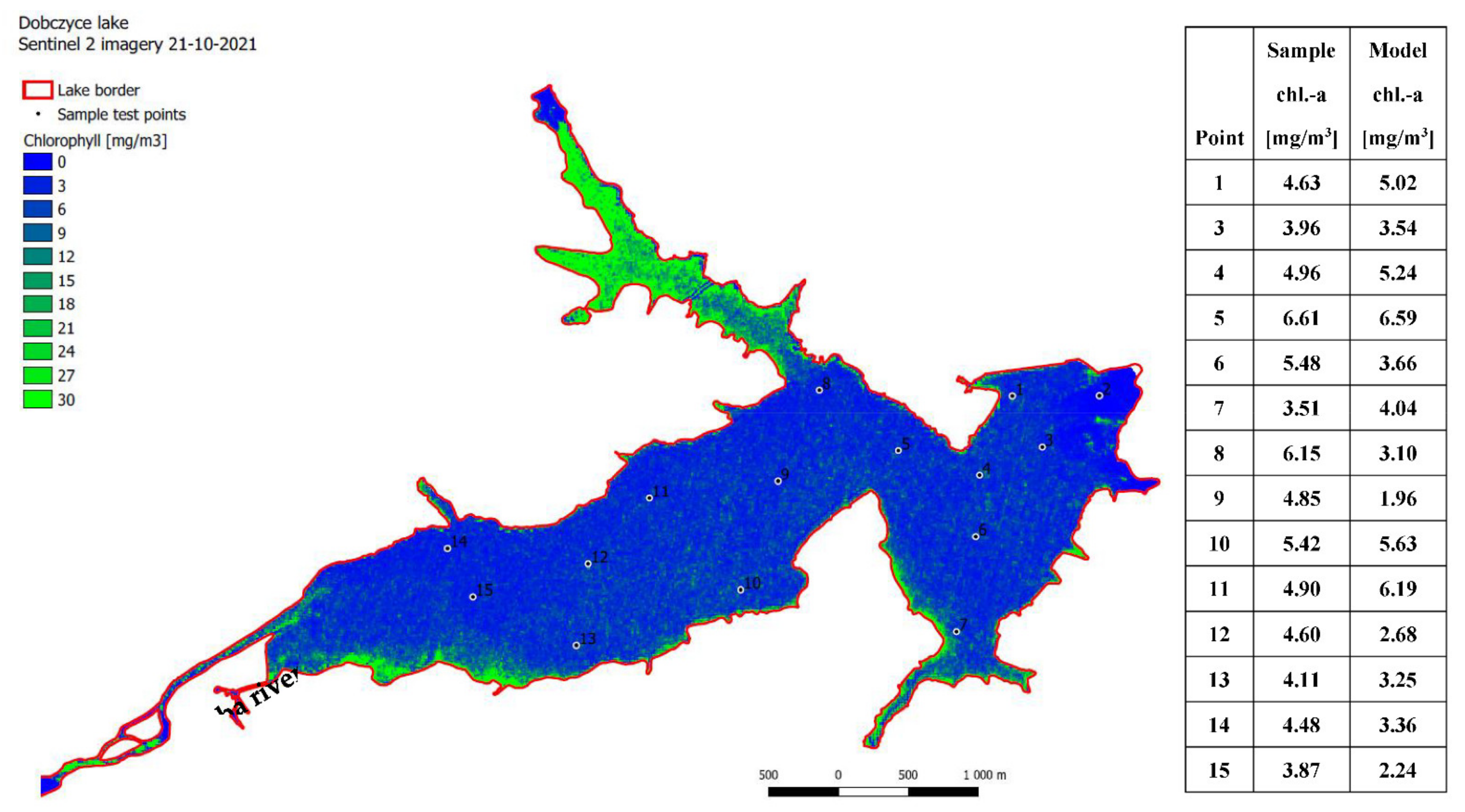
In October, water temperatures in the lake are low (around 13 °C), and the algae growth slows down. At that time, higher concentrations of algae could be found only in the northern branch of the lake (stagnant zone) and at the southern shores, where low flow velocities (Figure 17) are responsible for stagnant zones (Figure 18). The chlorophyll a model showed a good fit to the measurement data (Figure 18, table).

3.3. Models Parameters for Turbidity

The turbidity C model was developed similarly to the chlorophyll a model. At first, it was determined which factors from the range of a₀–a₁₆ are significant for turbidity in Equation (3). Then, the significance test was used for the a₁–a₁₆ coefficients at a significance level of 0.05 using the Student’s t-distribution. It was found that the most important coefficients are related to the wavelengths: 705, 740, and 783 nm; these lengths approximately correspond to the local minimum and maximum on the spectral curve of suspensions (Figure 2, Figure 3 and Figure 4). The initial form of the equation was as follows:

$$\begin{array}{l}\mathbf{ln}C=a_{C,0}+a_{C,4}\mathbf{ln}{R}_{705}+a_{C,5}\mathbf{ln}{R}_{740}+a_{C,6}\mathbf{ln}{R}_{783}+\\ a_{C,12}{\left(\mathbf{ln}{R}_{705}\right)}^2+a_{C,13}{\left(\mathbf{ln}{R}_{740}\right)}^2+a_{C,14}{\left(\mathbf{ln}{R}_{783}\right)}^2\end{array}$$

(16)

C—turbidity [NTU];

a_….—model coefficients;

R_….—radiation reflectance for wavelengths: 705, 740, and 783 nm.

Taking into account the reflectance of the lake bottom leads to a relationship:

$$\begin{array}{l}C=\mathbf{exp} a_{C,0}+a_{C,4}\mathbf{ln}\left(R_{705}-{\alpha }_{C,b,\hspace{0.33em}705}\mathbf{exp}\left(-k_{C,705}·C·2h\right)\right)+\\ a_{C,5}\mathbf{ln}{R}_{740}+a_{C,6}\mathbf{ln}{R}_{783}+\\ a_{C,12}{\left(\mathbf{ln}\left(R_{705}-{\alpha }_{C,b,\hspace{0.33em}705}\mathbf{exp}\left(-k_{C,705}^{}·C·2h\right)\right)\right)}^2+\\ a_{C,13}{\left(\mathbf{ln}{R}_{740}\right)}^2+a_{C,14}{\left(\mathbf{ln}{R}_{783}\right)}^2\end{array}$$

(17)

$\mathbf{exp}(a_{C,0})$—model’s coefficient [NTU].

The effect of light reflection by the lake bottom is shown in Figure 11. It appears that it is sufficient to consider the reflectance correction for 705 nm to obtain a satisfactory accuracy of model (17). Of course, it is also possible to correct the reflectance for 740 nm and 783 nm, but the overall improvement of the model quality would be negligible.

Equation (17) is implicit due to turbidity C. The C value can be obtained by successive approximations, i.e., inserting in $\mathbf{exp}\left(-k_{C,705}^{}·C·2h\right)$ values C from the previous approximation; after several attempts (e.g., 4), the value C becomes reasonably accurate. Another method involves searching for the function’s zero, i.e., the difference of the right side of Equation (17) and C. Here, the regula falsi method of searching for the function’s zero can be used.

Based on the measurement data of: turbidity C, lake depth h, and the reflectance R... for wavelengths 705, 740, and 783 nm, the parameters of model (17) were determined. Due to the large number of parameters:

$$a_{C,0}\hspace{0.33em},\hspace{0.33em}{a}_{C,4}\hspace{0.33em},\hspace{0.33em}{\alpha }_{C,b,\hspace{0.33em}705}\hspace{0.33em},\hspace{0.33em}{k}_{C,705}\hspace{0.33em},\hspace{0.33em}{a}_{C,5}\hspace{0.33em},\hspace{0.33em}{a}_{C,6}\hspace{0.33em},\hspace{0.33em}{a}_{C,12}\hspace{0.33em},\hspace{0.33em}{a}_{C,13}\hspace{0.33em},\hspace{0.33em}{a}_{C,14}$$

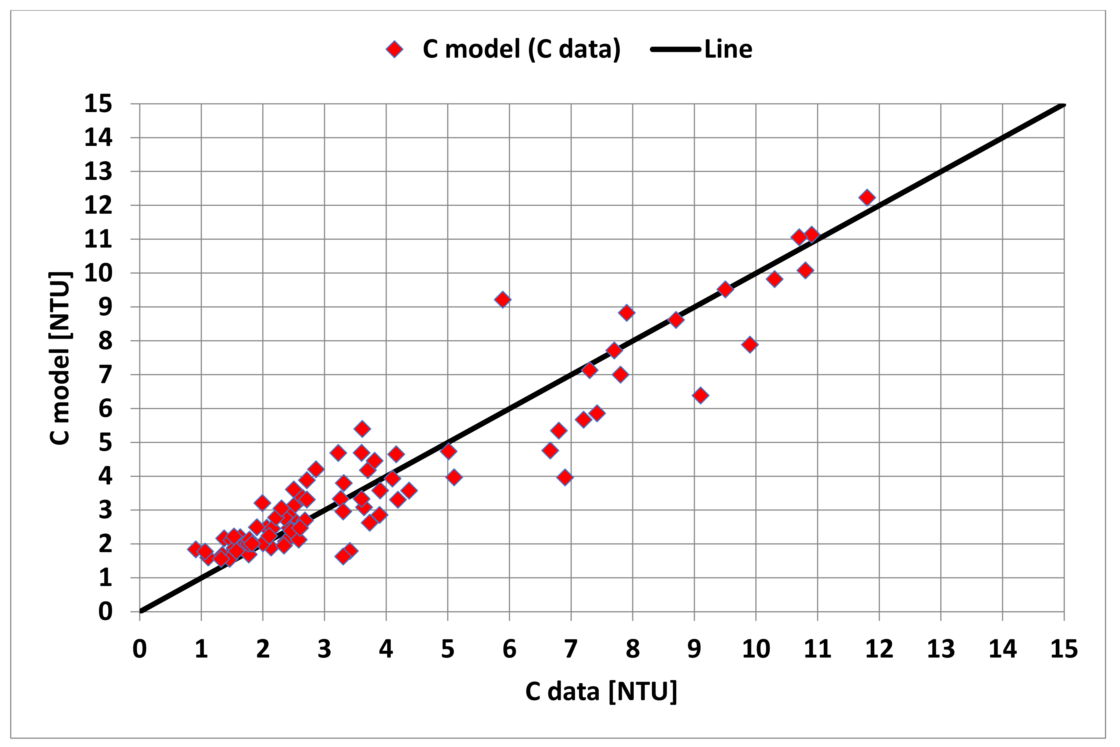
the two-stage procedure was employed. First, the values of some parameters were initially estimated: $a_{C,0}\hspace{0.33em},\hspace{0.33em}{a}_{C,4}\hspace{0.33em},\hspace{0.33em}{a}_{C,5}\hspace{0.33em},\hspace{0.33em}{a}_{C,6}\hspace{0.33em},\hspace{0.33em}{a}_{C,12}\hspace{0.33em},\hspace{0.33em}{a}_{C,13}\hspace{0.33em},\hspace{0.33em}{a}_{C,14}$, and then all the others were estimated, while correcting the values of the pre-estimated parameters. The parameters were determined using the least squares method (the best fit) for turbidity C and turbidity from model (17). The model parameters are summarized in

Table 3. Values of the model (17) parameters.

Parameter	Value	Unit
$a_{C,0}$	−28.87376959	ln(NTU)
$a_{C,4}$	13.12134743	–
${\alpha }_{C,b,\hspace{0.33em}705}$	0.014648999	–
$k_{C,705}$	0.0000434391	(NTU·m)−1
$a_{C,5}$	−59.94110417	–
$a_{C,6}$	26.75417218	–
$a_{C,12}$	1.323875637	–
$a_{C,13}$	−8.392820945	–
$a_{C,14}$	3.936558098	–

. The correlation coefficient was 0.939, and the model fit is shown in Figure 19. A good fit of the model to the measurement data was obtained.

3.4. Maps of Turbidity for Lake Dobczyce

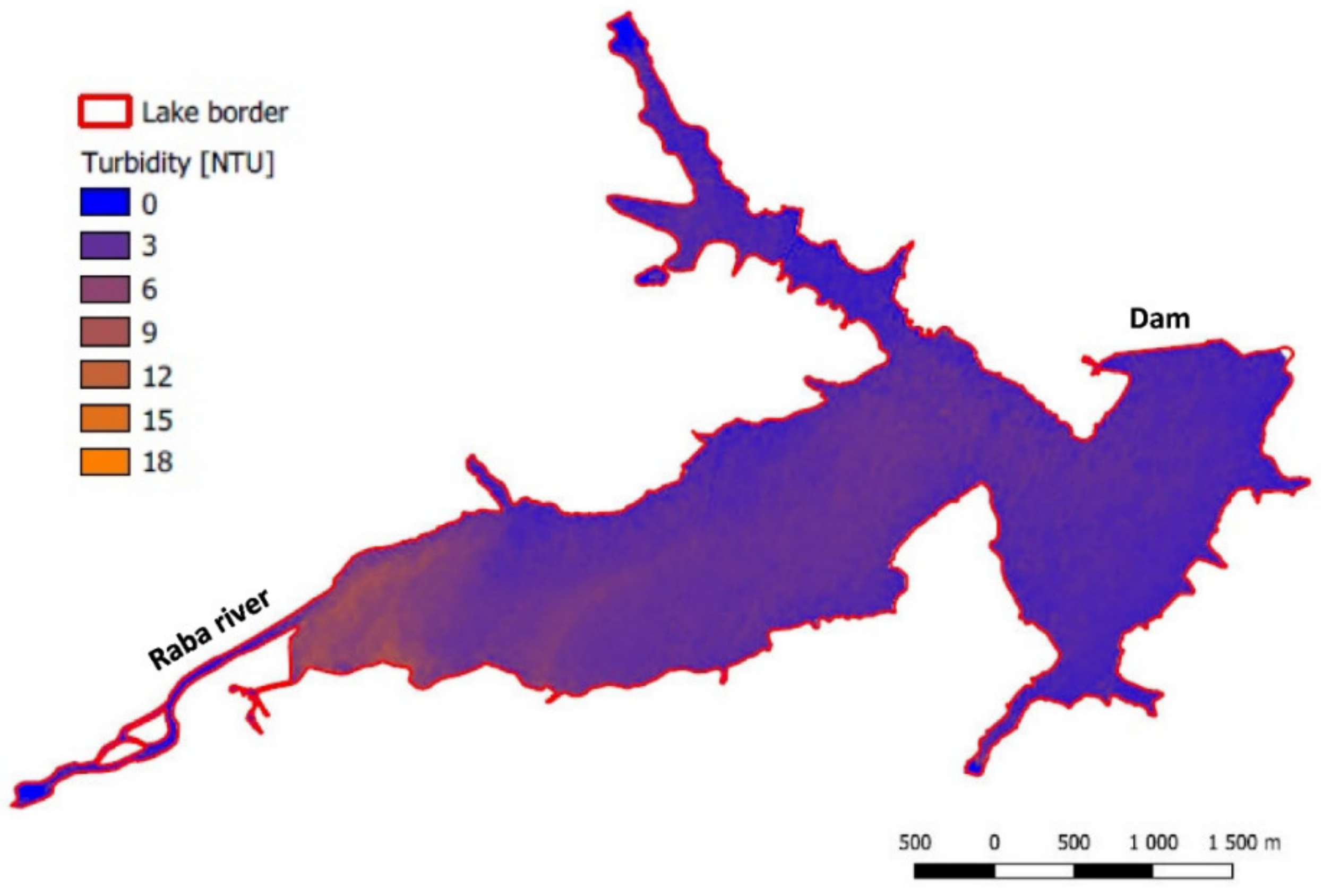
The water turbidity map for the lake (Figure 20) was developed from the satellite images and model (17). Long retention times in Lake Dobczyce (average 157 days) favor the sedimentation of suspended particles. Therefore, the water turbidity in the middle of the lake, towards the dam, where there are low velocities (Figure 17), is lower than turbidity close to the place where the Raba river enters the lake (Figure 20). In the branches of the lake, where water exchange is low and retention times are longer, low turbidity may be attributed to good sedimentation conditions (Figure 20); turbidity is also low on the south-eastern shores of the lake, where the flow velocities are low.

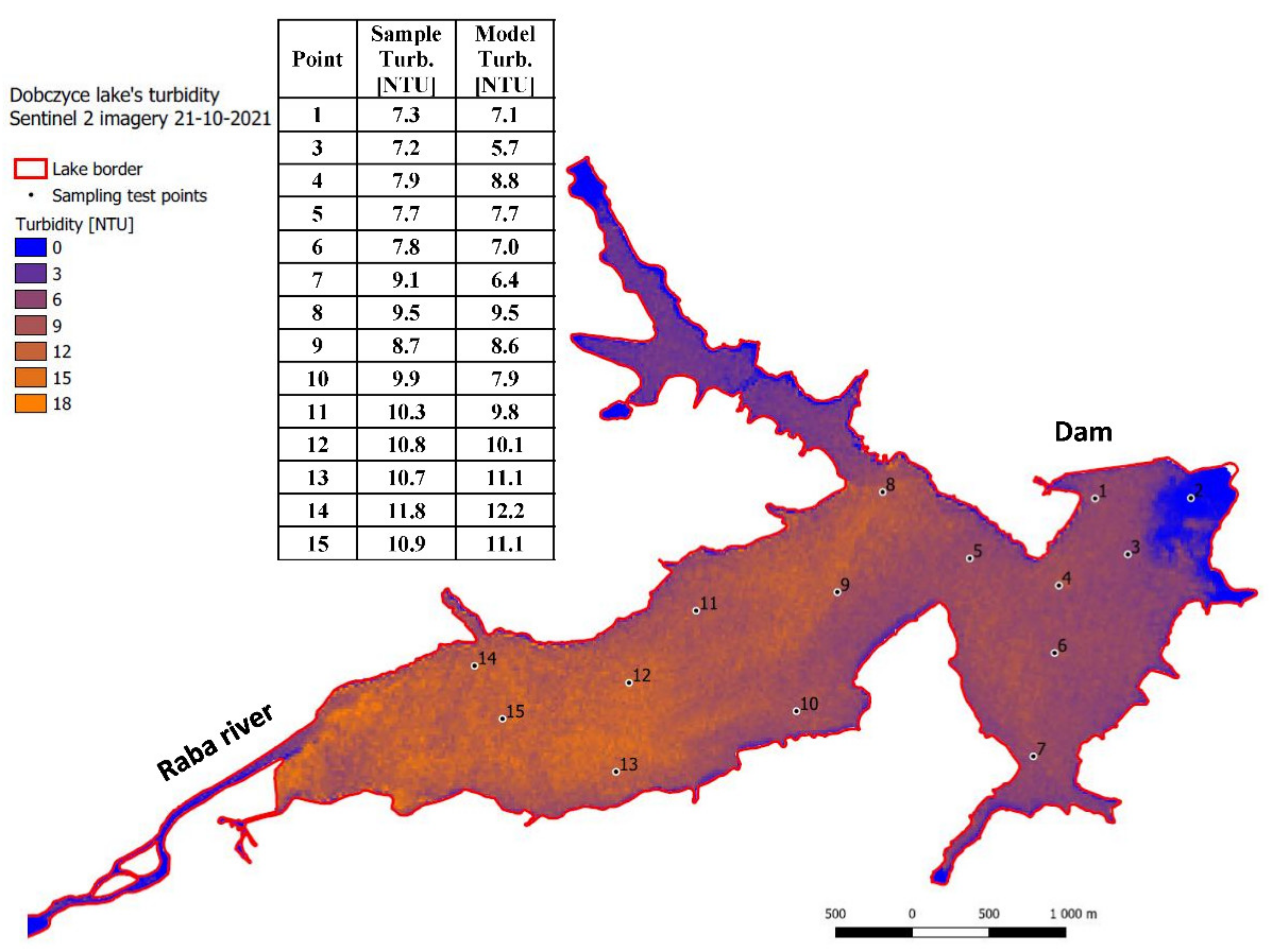
In October (Figure 21) and in May (Figure 20), turbidity decreased along the lake towards the dam. Moreover, in the northern branch, sedimentation contributed to a lower turbidity (Figure 21). The turbidity model showed a good fit with the measurements (Figure 21, table); however, at point 2 (Figure 21), the turbidity calculations were poor due to clouds obscuring the view.

4. Discussion

The authors developed the model to calculate the concentration of chlorophyll a and turbidity in the water. In the case of Lake Dobczyce, the chlorophyll a model takes into account reflectance corresponding to the middle wavelengths 665, 705, 740, and 842 nm, while the bottom effect is related to the wavelengths 665 and 705 nm. The model for turbidity considers the reflectance corresponding to the middle wavelengths 705, 740, and 783 nm, while the bottom effect is related to the wavelength 705 nm. To eliminate a minor reflectance related to other wavelengths from the pseudo-linear model (3), the Student’s t-test was been used for both chlorophyll a and turbidity. It cannot be predicted in advance whether the models for different lakes will always use the reflectance for the same wavelengths. If so, the model coefficients may probably be different due to different water characteristic and other properties of the bottom sediments. In the case of Lake Dobczyce, all of the discriminants that are quotients of reflectance differences or reflectance quotients (Table 1) were not used in the models because they did not improve their quality.

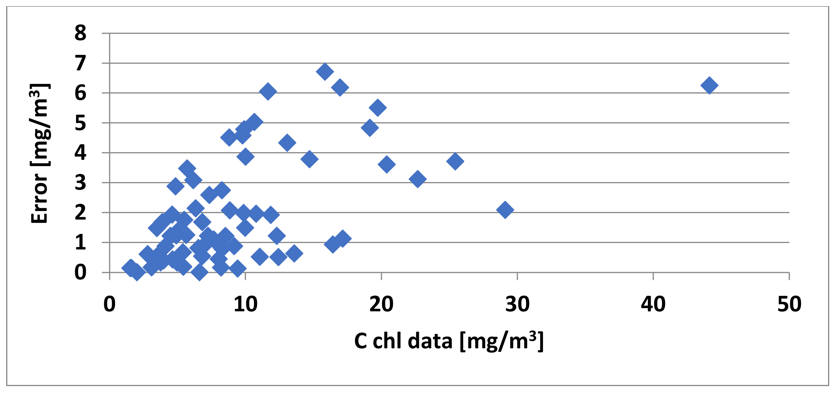
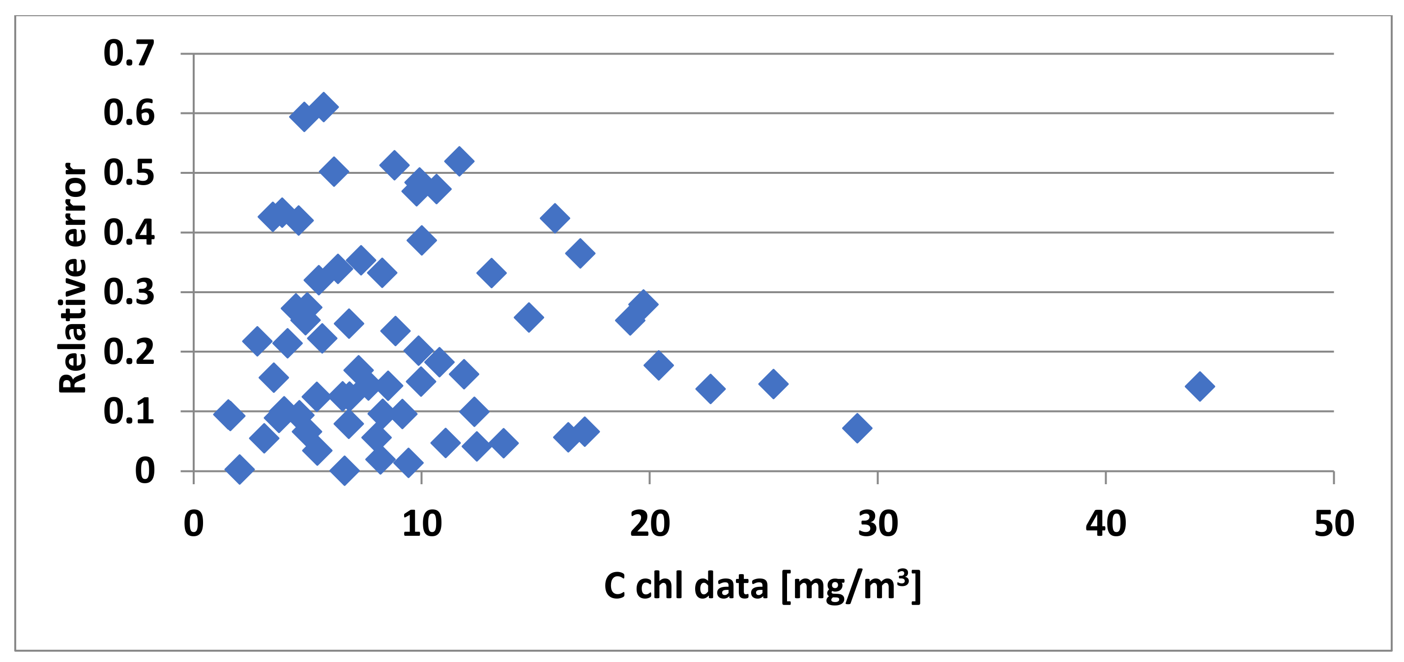
The average relative error of the model for chlorophyll a is about 0.216, while the average error is about 2.01 mg Chl a/m³. Graphs for errors are shown in Figure 22 and Figure 23.

The greatest errors of the model relate to concentrations of about 15 mg Chl a/m³ (Figure 22) and the highest relative errors concentrations of about 6 mg Chl a/m³ (Figure 23). For low and high chlorophyll a concentrations, the relative errors are the smallest. Sometimes, the existence of greater errors is caused by the unrepresentativeness of point measurement relative to the area represented by one raster. In addition, a greater number of data with average values of chlorophyll a concentration increases the likelihood of a greater error.

The reflectance corrections for 665 nm were smaller than for 705 nm (Figure 24). This may be due to the fact that the wavelength of emissions for chlorophyll a is 663 nm, after it was stimulated using a 430 nm radiation. Backscattering with a length of 665 nm, recorded by the satellite, therefore had to be more characteristic of chlorophyll a than for other substances contained in water. Backscattering with a length of 705 nm is characteristic of minerals, in particular montmorillonite (Figure 8), and this likely explains why the reflectance corrections were greater. Reflectances for other wavelengths, occurring in the model for chlorophyll a, can be characteristic of other substances contained in water and atmosphere ingredients.

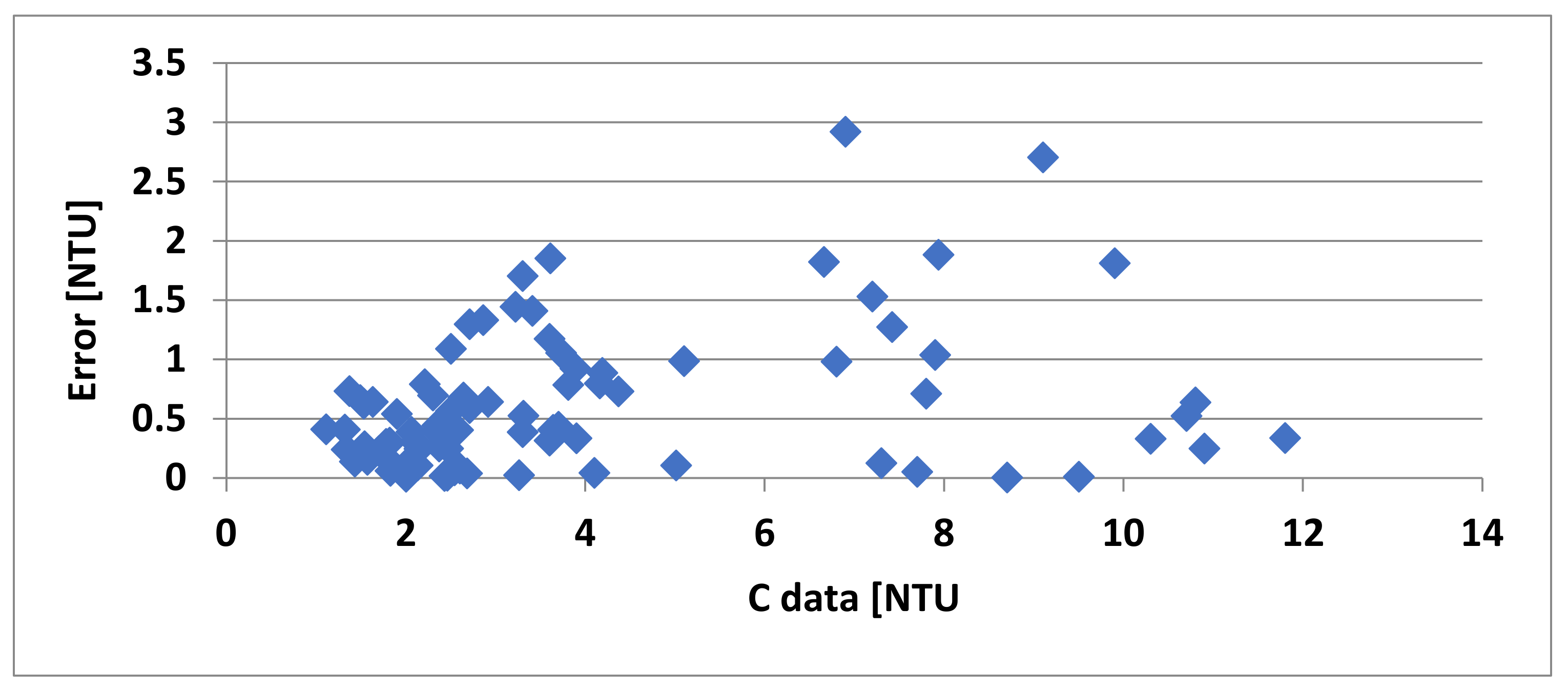
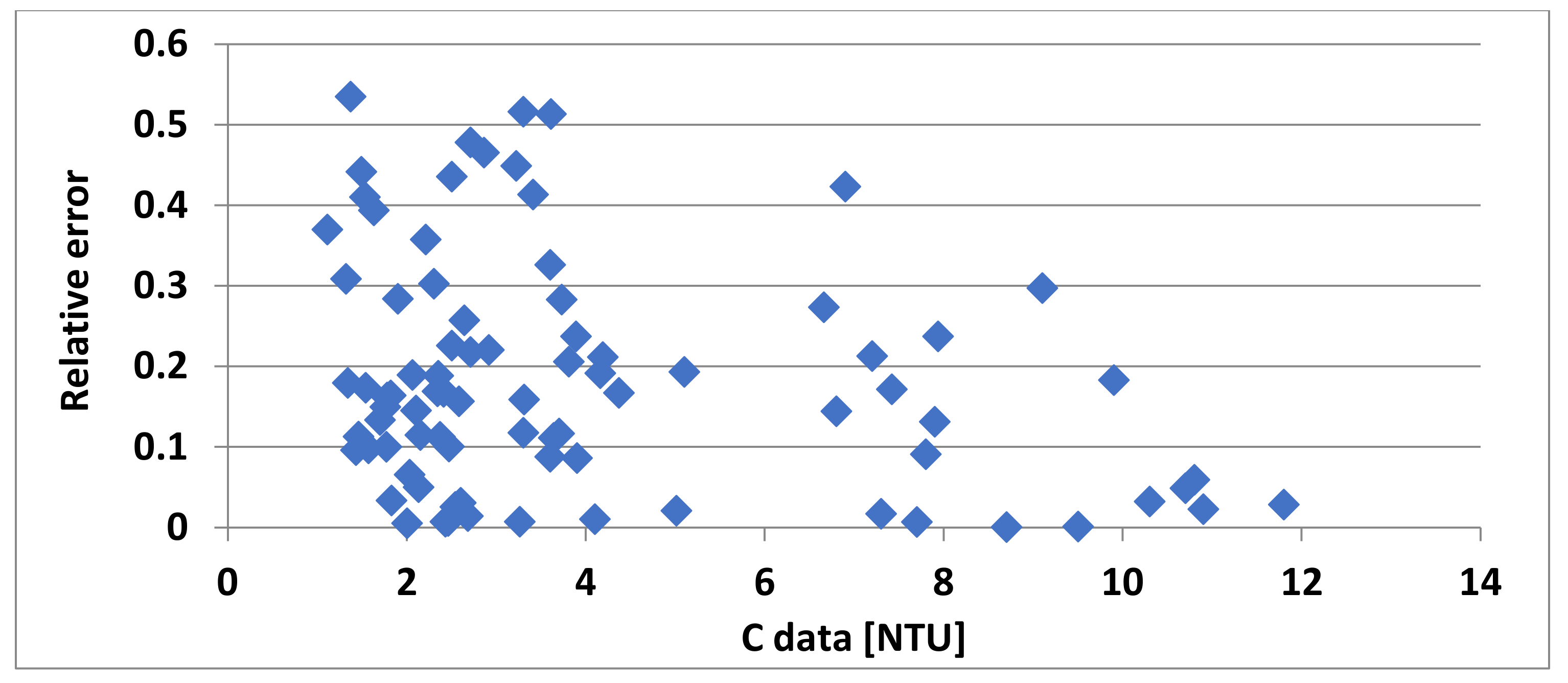
The average relative error of the model for turbidity is about 0.184, while the average error is about 0.629 NTU. Graphs of errors are shown in Figure 25 and Figure 26.

The greatest errors for the turbidity model concern the turbidity of about 7 NTU (Figure 25) and the greatest relative errors of turbidity of about 2–4 NTU (Figure 26). Sometimes, the existence of greater errors is caused by the unrepresentativeness of point measurement relative to the area represented by one raster. In addition, a greater number of data with average turbidity increases the likelihood of a greater error.

The reflectance corrections for 705 nm for the turbidity model were approximately constant and amounted to around 0.0146.

The remote determination of water quality parameters requires corrections of the reflectance measured by the satellite, which may pose some problems. In urbanized areas or areas close to industrial agglomerations, standard corrections do not give good results. The changes in composition of the atmosphere (content of moisture, dust, and other pollutants) may require different corrections. Therefore, it becomes necessary to determine a reference surface that enables a reflectance correction. This can be any surface with spectral properties constant in time. In this case, a fragment of the dam crest served as the reference surface. The base reflectance was the first reference surface reflectance in a series of measurements. The changes in the reflectance of the reference surface in relation to the base surface made it possible to correct the reflectance of the lake surface.

5. Conclusions

• The large number of different models used to calculate chlorophyll a concentrations and turbidity in water means that there is no one universal model for use with different bodies of water.
• Models developed as the product of the reflectance powers (after logarithm) undergo statistical analysis to eliminate irrelevant components. This procedure simplifies the model. The final model may take into account the reflectances of many wavelengths, which are then eliminated by the statistical test at the significance level, e.g., 0.05 (Student’s t-distribution).
• The specific physic-chemical and biological composition of the water in a given reservoir may result in significant differences between the spectral curves for individual water components.
• Shallow reservoirs require corrections for the bottom reflectance. It is impossible to predict in advance at what depth and for which wavelengths the bottom reflectance is already negligible. The analysis of satellite images helps to determine whether the bottom reflectance at a given wavelength is insignificant (poor bottom visibility); this simplifies the model.
• It is difficult or even impossible to use a combination of physical equations (type (7)–(9)) to calculate the concentration of chlorophyll a based on the reflectance recorded by the satellite; such reflectance is a mix of the chlorophyll a reflectance and the reflectance of many other substances present in the water. The authors could not find parameters of the model types (7)–(9) for just one wavelength and the known turbidity and maintain a satisfactory accuracy. Therefore, they proposed model (14) that took into account the reflectance for different wavelengths.
• Reflectances corresponding to the middle wave range 665, 705, 740, and 842 nm have been used in the model of chlorophyll concentration, while the effect of lake bottom interaction is associated with wavelengths 665 and 705 nm.
• Reflectances corresponding to the middle wave range 705, 740, and 783 nm have been used in the model of turbidity, while the effect of lake bottom interaction is associated with wavelength 705 nm.
• The described models use the reflectances normalized to the conditions prevailing at a specific moment over the reference surface.

References

- Clesceri, L.S.; Greenberg, A.E.; Eaton, A.D. Standard Methods for the Examination of Water and Wastewater, 20th ed.; APHA American Public Health Association: Washington, DC, USA, 1998. [Google Scholar]
- Aminot, A.; Rey, F. Standard Procedure for the Determination of Chlorophyll a by Spectroscopic Methods; International Council for the Exploration of the Sea: Copenhagen, Denmark, 2000; ISSN 0903-2606. Available online: https://www.researchgate.net/publication/242385183_Standard_procedure_for_the_determination_of_chlorophyll_a_by_spectroscopic_methods (accessed on 29 June 2022).
- Miller, H.M.; Sexton, N.R.; Koontz, L.; Loomis, J.; Koontz, S.R.; Hermans, C. USGS Open-File Report 2011-1031: The Users, Uses, and Value of Landsat and Other Moderate-Resolution Satellite Imagery in the United States—Executive Report. Available online: https://pubs.usgs.gov/of/2011/1031/ (accessed on 29 June 2022).
- Allan, M.G.; Hamilton, D.P.; Hicks, B.J.; Brabyn, L. Landsat Remote Sensing of Chlorophyll a Concentrations in Central North Island Lakes of New Zealand. Int. J. Remote Sens. 2011, 32, 2037–2055. [Google Scholar] [CrossRef]
- Ventura, D.L.T.; Martinez, J.-M.; de Attayde, J.L.; Martins, E.S.P.R.; Brandini, N.; Moreira, L.S. Long-Term Series of Chlorophyll-a Concentration in Brazilian Semiarid Lakes from Modis Imagery. Water 2022, 14, 400. [Google Scholar] [CrossRef]
- Albert, A.; Gege, P. Inversion of Irradiance and Remote Sensing Reflectance in Shallow Water between 400 and 800 Nm for Calculations of Water and Bottom Properties. Appl. Opt. 2006, 45, 2331–2343. [Google Scholar] [CrossRef] [PubMed]
- Richter, R.; Schläpfer, D. Atmospheric/Topographic Correction for Satellite Imagery; DLR Report DLR-IB 565–601: Wessling, Germany, 2005. [Google Scholar]
- Song, K. Water Quality Monitoring Using Landsat Themate Mapper Data with Empirical Algorithms in Chagan Lake, China. J. Appl. Remote Sens. 2011, 5, 053506. [Google Scholar] [CrossRef]
- Lim, J.; Choi, M. Assessment of Water Quality Based on Landsat 8 Operational Land Imager Associated with Human Activities in Korea. Environ. Monit. Assess. 2015, 187, 384. [Google Scholar] [CrossRef]
- Le, C.; Li, Y.; Zha, Y.; Sun, D.; Huang, C.; Lu, H. A Four-Band Semi-Analytical Model for Estimating Chlorophyll a in Highly Turbid Lakes: The Case of Taihu Lake, China. Remote Sens. Environ. 2009, 113, 1175–1182. [Google Scholar] [CrossRef]
- Kudela, R.M.; Palacios, S.L.; Austerberry, D.C.; Accorsi, E.K.; Guild, L.S.; Torres-Perez, J. Application of Hyperspectral Remote Sensing to Cyanobacterial Blooms in Inland Waters. Remote Sens. Environ. 2015, 167, 196–205. [Google Scholar] [CrossRef] [Green Version]
- Peterson, K.T.; Sagan, V.; Sloan, J.J. Deep Learning-Based Water Quality Estimation and Anomaly Detection Using Landsat-8/Sentinel-2 Virtual Constellation and Cloud Computing. GISci. Remote Sens. 2020, 57, 510–525. [Google Scholar] [CrossRef]
- Sagan, V.; Peterson, K.T.; Maimaitijiang, M.; Sidike, P.; Sloan, J.; Greeling, B.A.; Maalouf, S.; Adams, C. Monitoring Inland Water Quality Using Remote Sensing: Potential and Limitations of Spectral Indices, Bio-Optical Simulations, Machine Learning, and Cloud Computing. Earth-Sci. Rev. 2020, 205, 103187. [Google Scholar] [CrossRef]
- IOCCG. Remote Sensing of Inherent Optical Properties: Fundamentals, Tests of Algorithms, and Applications; International Ocean Colour Coordinating Group (IOCCG): Dartmouth, NS, Canada, 2006; ISSN 1098-6030. Available online: https://www.ioccg.org/reports/report5.pdf (accessed on 1 January 2022).
- Li, Y.; Shang, S.; Zhang, C.; Ma, X.; Huang, L.; Wu, J.; Zeng, Y. Remote Sensing of Algal Blooms Using a Turbidity-Free Function for near-Infrared and Red Signals. Chin. Sci. Bull. 2006, 51, 464–471. [Google Scholar] [CrossRef]
- Schalles, J.F.; Schiebe, F.R.; Starks, P.J.; Troeger, W.W. Estimation of Algal and Suspended Sediment Loads (singly and Combined) Using Hyperspectral Sensors and Integrated Mesocosm Experiments. In Proceedings of the Fourth International Conference on Remote Sensing for Marine and Coastal Environments, Orlando, FL, USA, 17–19 March 1997; pp. 111–120. [Google Scholar]
- Ritchie, J.C.; Zimba, P.V.; Everitt, J.H. Remote Sensing Techniques to Assess Water Quality. Photogramm. Eng. Remote Sens. 2003, 69, 695–704. [Google Scholar] [CrossRef] [Green Version]
- Lodhi, M.A.; Rundquist, D.C.; Han, L.; Kuzila, M.S. The Potential for Remote Sensing of Loess Soils Suspended in Surface Waters. J. Am. Water Resour. Assoc. 1997, 33, 111–117. [Google Scholar] [CrossRef]
- Alparslan, E.; Aydöner, C.; Tufekci, V.; Tüfekci, H. Water Quality Assessment at Ömerli Dam Using Remote Sensing Techniques. Environ. Monit. Assess. 2007, 135, 391. [Google Scholar] [CrossRef] [PubMed]
- Johan, F.B.; Jafri, M.Z.B.; San, L.H.; Omar, W.M.W.; Ho, T.C. Chlorophyll a Concentration of Fresh Water Phytoplankton Analysed by Algorithmic Based Spectroscopy. J. Phys. Conf. Ser. 2018, 1083, 012015. [Google Scholar] [CrossRef] [Green Version]
- Gitelson, A.A.; Dall’Olmo, G.; Moses, W.; Rundquist, D.C.; Barrow, T.; Fisher, T.R.; Gurlin, D.; Holz, J. A Simple Semi-Analytical Model for Remote Estimation of Chlorophyll-a in Turbid Waters: Validation. Remote Sens. Environ. 2008, 112, 3582–3593. [Google Scholar] [CrossRef]
- Shen, F.; Zhou, Y.-X.; Li, D.-J.; Zhu, W.-J.; Salama, M.S. Medium Resolution Imaging Spectrometer (MERIS) Estimation of Chlorophyll-a Concentration in the Turbid Sediment-Laden Waters of the Changjiang (Yangtze) Estuary. Int. J. Remote Sens. 2010, 31, 4635–4650. [Google Scholar] [CrossRef]
- Son, S.; Wang, M. Water Quality Properties Derived from VIIRS Measurements in the Great Lakes. Remote Sens. 2020, 12, 1605. [Google Scholar] [CrossRef]
- Diouf, D.; Seck, D. Modeling the Chlorophyll-a from Sea Surface Reflectance in West Africa by Deep Learning Methods: A Comparison of Multiple Algorithms. Int. J. Artif. Intell. Appl. 2019, 10, 33–40. [Google Scholar] [CrossRef]
- Johnson, R.; Strutton, P.G.; Wright, S.W.; McMinn, A.; Meiners, K.M. Three Improved Satellite Chlorophyll Algorithms for the Southern Ocean. J. Geophys. Res. Ocean. 2013, 118, 3694–3703. [Google Scholar] [CrossRef]
- Hansen, C.H.; Williams, G.P.; Adjei, Z.; Barlow, A.; Nelson, E.J.; Miller, A.W. Reservoir Water Quality Monitoring Using Remote Sensing with Seasonal Models: Case Study of Five Central-Utah Reservoirs. Lake Reserv. Manag. 2015, 31, 225–240. [Google Scholar] [CrossRef]
- Mobley, C.D. Hydrolight 3.1 Users’ Guide. 1996. Available online: https://apps.dtic.mil/sti/pdfs/ADA356954.pdf (accessed on 1 January 2022).
- Salama, M.S.; Verhoef, W. Two-Stream Remote Sensing Model for Water Quality Mapping: 2SeaColor. Remote Sens. Environ. 2015, 157, 111–122. [Google Scholar] [CrossRef]
- Cannizzaro, J.P.; Carder, K.L. Estimating Chlorophyll a Concentrations from Remote-Sensing Reflectance in Optically Shallow Waters. Remote Sens. Environ. 2006, 101, 13–24. [Google Scholar] [CrossRef]
- Werdell, P.J.; Jeremy Werdell, P.; Roesler, C.S. Remote Assessment of Benthic Substrate Composition in Shallow Waters Using Multispectral Reflectance. Limnol. Oceanogr. 2003, 48, 557–567. [Google Scholar] [CrossRef] [Green Version]
- Hicks, B.J.; Stichbury, G.A.; Brabyn, L.K.; Allan, M.G.; Ashraf, S. Hindcasting Water Clarity from Landsat Satellite Images of Unmonitored Shallow Lakes in the Waikato Region, New Zealand. Environ. Monit. Assess. 2013, 185, 7245–7261. [Google Scholar] [CrossRef] [PubMed]
- Li, J.; Yu, Q.; Tian, Y.Q.; Becker, B.L. Remote Sensing Estimation of Colored Dissolved Organic Matter (CDOM) in Optically Shallow Waters. ISPRS J. Photogramm. Remote Sens. 2017, 128, 98–110. [Google Scholar] [CrossRef] [Green Version]
- Li, J.; Yu, Q.; Tian, Y.Q.; Becker, B.L.; Siqueira, P.; Torbick, N. Spatio-Temporal Variations of CDOM in Shallow Inland Waters from a Semi-Analytical Inversion of Landsat-8. Remote Sens. Environ. 2018, 218, 189–200. [Google Scholar] [CrossRef]
- Lee, Z.; Carder, K.L.; Mobley, C.D.; Steward, R.G.; Patch, J.S. Hyperspectral Remote Sensing for Shallow Waters. 2. Deriving Bottom Depths and Water Properties by Optimization. Appl. Opt. 1999, 38, 3831–3843. [Google Scholar] [CrossRef] [Green Version]
- Lee, Z.; Carder, K.L.; Mobley, C.D.; Steward, R.G.; Patch, J.S. Hyperspectral Remote Sensing for Shallow Waters. I. A Semianalytical Model. Appl. Opt. 1998, 37, 6329–6338. [Google Scholar] [CrossRef]
- Śliwiński, D.; Konieczna, A.; Roman, K. Geostatistical Resampling of LiDAR-Derived DEM in Wide Resolution Range for Modelling in SWAT: A Case Study of Zgłowiączka River (Poland). Remote Sens. 2022, 14, 1281. [Google Scholar] [CrossRef]
- PN-EN ISO 7027-1:2016-09; Water Quality—Determination of Turbidity (ISO_7027:1999). Polish Committee for Standardization EN_ISO_7027:1999: Warsaw, Poland, 2016.
- PN-86/C-05560/02; Water and Sewage. Polish Committee for Standardization: Warsaw, Poland, 1986. Available online: https://www.ydylstandards.org.cn/static/down/pdf/PN%20C05560-02-1986_0000.pdf (accessed on 1 January 2022).
- Kokaly, R.F.; Clark, R.N.; Swayze, G.A.; Livo, K.E.; Hoefen, T.M.; Pearson, N.C.; Wise, R.A.; Benzel, W.M.; Lowers, H.A.; Driscoll, R.L.; et al. USGS Spectral Library Version 7; U.S. Geological Survey Data Series 1035; U.S. Geological Survey: Reston, VA, USA, 2017; 61p. [CrossRef]
- Hachaj, P.S. Analysis of Hydrodynamics of Barrier Reservoirs for the Needs of Water Management: Model and Its Application; Cracow University of Technology: Kraków, Poland, 2019; ISBN 9788365991614. [Google Scholar]
Figure 1.
Surface remote sensing reflectance spectrum for the waters with different concentration of chlorophyll a, collected in the study area (119°52′–119°54′ E, 26°16′–26°19′ N) at 10:00–15:40, 2 June 2003. Reprinted with permission from [15].
Figure 2.
Relative contributions of chlorophyll and suspended sediment to a reflectance spectra of the surface water, based on in situ laboratory measurements made 1 m above the water surface by the authors of [16,17]. Reprinted with permission from [16,17].
Figure 3.
Reflectance for water with a clay suspension [g/m3]. Reprinted with permission from [18].
Figure 4.
Reflectance for water with a dusty suspension [g/m3]. Reprinted with permission from [18].
Figure 5.
Depth map of Lake Dobczyce.
Figure 6.
Some spectral curves for the fragment of the dam crest.
Figure 7.
Reflectance at different measuring points of Lake Dobczyce in the years 2016–2021, after a normalization of the original reflectance from the satellite.
Figure 8.
Spectral curve for the montmorillonite suspensions in water, USGS Spectral Library Version 7, https://crustal.usgs.gov/speclab/QueryAll07a.php?quick_filter=water (accessed on 1 January 2022). Reprinted with permission from [39].
Figure 9.
Spectral curve of chlorophyll in water (2.97 mg chl/m3), USGS Spectral Library Version 7, https://crustal.usgs.gov/speclab/QueryAll07a.php?quick_filter=water (accessed on 1 January 2022). Reprinted with permission from [39].
Figure 10.
Spectral curve of chlorophyll in water (7.609 mg chl/m3), USGS Spectral Library Version 7, https://crustal.usgs.gov/speclab/QueryAll07a.php?quick_filter=water (accessed on 1 January 2022). Reprinted with permission from [39].
Figure 11.
Images of Lake Dobczyce at four wavelengths (color representation: blue, yellow, violet, with the same color saturation in each photo).
Figure 12.
Changes in reflectance R as a function of depth h for the sensor above the water surface at different concentrations of chlorophyll a = {1, 5, 10, 20, 50} mg/m3.
Figure 13.
Chlorophyll a Cchl concentrations as a function of depth h for Equations (7)–(9) and model (15) (approximation).
Figure 14.
Model fit (Cchl model) (14) to the measured concentrations of chlorophyl-a (Cchl data) at the known turbidity values.
Figure 15.
Model fit (Cchl model) (14) to the measured concentrations of chlorophyl-a (Cchl data) for turbidity model (17).
Figure 16.
Chlorophyll concentration in Lake Dobczyce 9 May2021 (imagery by Sentinel 2).
Figure 17.
Two-dimensional field of the average vertical velocity in the main part of Lake Dobczyce (without the northern bay), with the total flow of 10 m3/s and no-wind conditions (model RMA2). Reprinted with permission from [40].
Figure 18.
Chlorophyll concentrations in Lake Dobczyce, 21 October 2021 (imagery by Sentinel 2).
Figure 19.
Model (17) fit (C model) to the measured turbidity (C data).
Figure 20.
Water turbidity of Lake Dobczyce 9 May 2021 (imagery by Sentinel 2).
Figure 21.
Water turbidity of Lake Dobczyce, 21 October 2021 (imagery by Sentinel 2).
Figure 22.
Model errors for chlorophyll a versus measurement data.
Figure 23.
Model relative errors for chlorophyll a versus measurement data.
Figure 24.
The reflection corrections graph versus the product of the depth and turbidity for the chlorophyll a model.
Figure 25.
Model errors for turbidity versus measurement data.
Figure 26.
Model relative errors for turbidity versus measurement data.