Position Control of a Mobile Robot through Deep Reinforcement Learning

Abstract

This article proposes the use of reinforcement learning (RL) algorithms to control the position of a simulated Kephera IV mobile robot in a virtual environment. The simulated environment uses the OpenAI Gym library in conjunction with CoppeliaSim, a 3D simulation platform, to perform the experiments and control the position of the robot. The RL agents used correspond to the deep deterministic policy gradient (DDPG) and deep Q network (DQN), and their results are compared with two control algorithms called Villela and IPC. The results obtained from the experiments in environments with and without obstacles show that DDPG and DQN manage to learn and infer the best actions in the environment, allowing us to effectively perform the position control of different target points and obtain the best results based on different metrics and indices.

1. Introduction

Mobile robots are widely used today and allow for the performance of tasks in environments dangerous for humans—for example, minefields, radioactive areas, deep-sea exploration, etc.—and for access to complex places, such as extraterrestrial exploration and nanorobotics in medicine [1]. The main problem lies in the need for these robots to be able to move around the environment with some autonomy such that they do not require human interaction—that is, they can be controlled automatically by their own intelligent systems to allow them to achieve certain objectives [2].

By combining control and robotics, different strategies can be provided that allow for the efficient control of mobile robots. The foregoing is represented by the use of control algorithms, such as Villela [3] and IPC [4], which seek to manipulate the speeds of the robot by controlling its linear and angular speed. To these algorithms, other systems can be added to strengthen their tasks—for example, obstacle avoidance systems through the use of sensor arrays arranged in the robot [5] and line trackers to improve position control [6,7]. In the previous cases, models of the feedback system are used that allow for the modification of a control law through inputs to calculate the next action and gradually decrease the error associated with its measurements. Additionally, different approaches are available, such as finite-time adaptive fault-tolerant control [8] and adaptive fuzzy control algorithms [9], which have been used for nonlinear systems in mobile robotics, as in [10].

Reinforcement learning (RL) is an area of machine learning that has its origins in the psychological and neuroscientific perspectives of animal behavior [11], where an agent learns to behave in an environment by performing actions and seeing the results of these actions in order to obtain the best expected result. Reinforcement learning has been used to solve different tasks—for example, in games obtaining high performance, as in Go [12], Starcraft [13] and Dota [14]. In the pursuit of making a general-purpose algorithm, DeepMind presented the MuZero [15] agent, which is capable of solving different games such as Go, Chess, Shogi and Atari. RL has been implemented in robotic systems for the precise manipulation of objects [16,17], and it has also been used to study how to transfer the training learned in simulation to reality (Sim-to-Real) [18,19,20].

Currently, RL is a widely used approach for robot control, and, regarding position control in mobile robots, it has been analyzed in [21,22], where they compare the results with control algorithms. Obstacle evasion has also been studied using different techniques from RL. For example, in [23], the Q-learning algorithm [24] is used, which bases its operation on the use of matrices (Q tables); thus, according to the state in which one is within the environment, observe which action has the best quality, that is, which one delivers the best reward. In [25,26], the neural Q-learning algorithm [27] is used, an approach quite similar to the previous one but which includes the use of neural networks as a nonlinear approximation to obtain the Q-values. In [28,29,30], different approaches of path planning with reinforcement learning are used, and in [31], a mixture of Q-learning and a neural network planner is used to solve route path planning problems. In [32], a version of the deep deterministic policy gradient (DDPG) [33] is implemented, which is used when the environment has a continuous action space. The indicated methods attempt to improve classical path-planning algorithms such as Dijkstra [34], BUG1 and BUG2 [35], and A* [36] has also been used for the navigation task.

In this work, we propose the development of an environment to control the position of the simulated mobile robot Khepera IV [37] by using two algorithms of the state of the art of RL—the deep Q-network (DQN) [38] and the deep deterministic policy gradient (DDPG)—and two control algorithms: Villela and IPC. The environment will be made using the CoppeliaSim simulation program (V-REP) [39] and the OpenAI Gym [40] library. The objective of the work is to adopt two known RL methods (DDPG and DQN) for the control of a simulated mobile robot and to compare the effectiveness of these methods with two known control methods. Several experiments to control the position of the mobile robot in environments with and without obstacles—and with one or more target points—will be performed. The results of the experiments will finally be compared by using various graphs and performance indices.

2. Reinforcement Learning

Reinforcement learning corresponds to a computational approach that allows for learning through interactions with the environment, which follows the structure given in the diagram in Figure 1. In machine learning, the environment is formulated as a Markov decision process, MDP [41], and allows us to obtain an idealized mathematical model that seeks to solve the learning problem through the interactions of an agent with an observable environment to achieve a goal.

The apprentice agent is responsible for making decisions. This apprentice interacts with an environment that responds to the actions taken and presents new situations to the agent. The environment also delivers a reward: a special numerical value that the agent seeks to maximize over time through decision making.

According to [42], the agent and the environment interact for each discrete time step $t$. As seen in Figure 1, the agent receives an observation or state of the environment, with which the agent selects an action within the set of actions allowed by the environment. Given this action, the agent receives a reward and a new state. At each time step, the agent performs a “mapping” of the states of the probability of selecting one of the possible actions. This task is called agent policy and is represented as ${\pi }_t$.

One of the problems to be addressed in RL is the “exploration/exploitation trade-off”, which occurs in learning systems that have to repeatedly decide on the basis of uncertain information. In essence, the dilemma lies in choosing whether to repeat decisions that have worked well so far (exploiting the information already obtained) or to make novel decisions in the hope of obtaining even greater rewards (exploring new possibilities) [43].

This article proposes the use of two deep reinforcement learning agents called deep Q-networks (DQNs) and deep deterministic policy gradients (DDPGs), which will be studied and analyzed as an alternative to mobile robotics problems, where control methods are usually used.

2.1. Deep Q-Network (DQN)

The DQN algorithm is an application of the Q-learning algorithm that uses neural networks. Through interaction with the environment, it is sought that the agent can maximize the future accumulated reward, which is achieved by occupying neural networks to optimally approximate the action-value function (Equation (1)), which is responsible for maximizing the sum of the reward $r$ discounted by $\gamma$; thus, as the time step $t$ increases, future rewards are increasingly less likely to occur.

$$Q^{*}\left(s,a\right)=\underset{\pi }{\max } E\left[r_t+\gamma r_{t+1}+{\gamma }^2{r}_{t+2}+\dots |s_t=s, a_t=a,\pi \right]$$

(1)

where $a$ is an action, $s$ is the current state and $\gamma \in \left[0,1\right]$ and $\pi$ are policies that map the agent’s behavior $\left(\pi =P\left(a|s\right)\right)$. A pseudoexplanatory code of the algorithms is presented in Algorithm 1. To address the effect of the “Exploration/Exploitation trade-off”, Epsilon Greedy can be used; Epsilon refers to the probability of choosing between exploring or exploiting, where most of the time the probability of exploring is low.

Algorithm 1 Deep Q-Learning algorithm with Experience Replay [44]

$\mathrm{Initialize} \mathrm{replay} \mathrm{memory} D$$\mathrm{to} \mathrm{capacity} N$ $\mathrm{Initialize} \mathrm{action}-\mathrm{value} \mathrm{function} Q$$\mathrm{with} \mathrm{random} \mathrm{weights} \theta$ $\mathrm{Initialize} \mathrm{target} \mathrm{action}-\mathrm{value} \mathrm{function} \widehat{Q}$$\mathrm{with} \mathrm{weights} {\theta }^{-}=\theta$ $\mathbf{for} \mathrm{episode}=1, M$do  $\mathrm{Initialize} \mathrm{sequence} s_1=\left\{x_1\right\}$$\mathrm{and} \mathrm{preprocessed} \mathrm{sequenced} {\mathsf{\varphi }}_1=\mathsf{\varphi }\left({\mathrm{s}}_1\right)$  $\mathbf{for} t=1, T$ do   $\mathrm{With}$$\mathrm{select} \mathrm{a} \mathrm{random} \mathrm{action} a_t$   $\mathrm{Otherwise}, \mathrm{select} a_t=argma{x}_{a}Q\left(\mathsf{\varphi }\left(s_t\right),a;\theta \right)$   $\mathrm{Execute} \mathrm{action} a_t$$\mathrm{in} \mathrm{simulation} \mathrm{and} \mathrm{observe} \mathrm{reward} r_t$$\mathrm{and} \mathrm{image} x_{t+1}$   $\mathrm{Set} s_{t+1}=s_t,a_t,x_{t+1}$$\mathrm{and} \mathrm{preprocess} {\mathsf{\varphi }}_{t+1}=\mathsf{\varphi }\left(s_{t+1}\right)$   $\mathrm{Store} \mathrm{transition} \left({\mathsf{\varphi }}_t,a_t,r_t,{\mathsf{\varphi }}_{t+1}\right)$$\mathrm{in} D$   $\mathrm{Sample} \mathrm{random} \mathrm{minibatch} \mathrm{of} \mathrm{transitions} \left({\mathsf{\varphi }}_j,a_j,r_j,{\mathsf{\varphi }}_{j+1}\right)$$\mathrm{from} D$   $\mathrm{Set} y_j=\{\begin{array}{c}\begin{array}{cc}{r}_j& if episode terminates at step j+1\end{array}\\ \begin{array}{cc}{r}_j+\gamma \underset{a^{\prime }}{\max }\widehat{Q} \left({\mathsf{\varphi }}_j,a_j;\theta \right)& otherwise\end{array}\end{array}$   $\mathrm{Perform} \mathrm{a} \mathrm{gradient} \mathrm{descent} \mathrm{step} \mathrm{on} {\left(y_j-Q\left({\mathsf{\varphi }}_j,a_j;\theta \right)\right)}^2$   $\mathrm{with} \mathrm{respect} \mathrm{to} \mathrm{the} \mathrm{network} \mathrm{parameters} \theta$   $\mathrm{Every}$$\mathrm{steps}, \mathrm{reset} \widehat{Q}=Q$  end for end for

2.2. Deep Deterministic Policy Gradient (DDPG)

The deep deterministic policy gradient (DDPG) agent is an off-policy algorithm and can be considered as a DQN for continuous action spaces. This agent uses two neural networks, one of which is called Actor and is in charge of learning the action policy ($\mu$), and the other is called Critic and works as an approximation of the Q-function. The policy is deterministic given that the action is to be performed directly, without the need to make an argmax of the Q-values, as is carried out in DQN. A pseudoexplanatory code of the DDPG algorithm is presented in Algorithm 2.

Algorithm 2 Deep Deterministic Policy Gradient algorithm [33]

$\mathrm{Randomly} \mathrm{initialize} \mathrm{critic} \mathrm{network} Q\left(s,a|{\theta }^Q\right)$$\mathrm{and} \mathrm{actor} \mu \left(s|{\theta }^{\mu }\right)$with weights ${\theta }^Q$$\mathrm{and} {\theta }^{\mu }$, respectively $\mathrm{Initialize} \mathrm{target} \mathrm{network} Q^{\prime }$$\mathrm{and} {\mu }^{\prime }$$\mathrm{with} \mathrm{weight} {\theta }^{Q^{\prime }}\leftarrow {\theta }^Q,{\theta }^{{\mu }^{\prime }}\leftarrow {\theta }^{\mu }$ $\mathrm{Initialize} \mathrm{replay} \mathrm{buffer} R$  $\mathbf{for} \mathrm{episode}=1, M$do  $\mathrm{Initialize} \mathrm{a} \mathrm{random} \mathrm{process} N$ for action exploration  $\mathrm{Receive} \mathrm{initial} \mathrm{observation} \mathrm{state} s_1$  $\mathbf{for} t=1, T$ do   $\mathrm{Select} \mathrm{action} a_t=\mu \left(s_t{|\theta }^{\mu }\right)+N_t$ according to the current policy and exploration noise   $\mathrm{Execute} \mathrm{action} a_t$ and observe reward and observe new state   $\mathrm{Store} \mathrm{transition} \left(s_t,a_t,r_t,s_{t+1}\right)$$\mathrm{in} R$   $\mathrm{Sample} \mathrm{a} \mathrm{random} \mathrm{minibatch} \mathrm{of} N$$\mathrm{transitions} \left(s_i,a_i,r_i,s_{i+1}\right)$$\mathrm{from} R$   $\mathrm{Set} y_i=r_i+\gamma Q^{\prime }\left(s_{i+1},{\mu }^{\prime }\left(s_{i+1}{|\theta }^{ {\mu }^{\prime }}\right){|\theta }^{Q^{\prime }}\right)$   $\mathrm{Update} \mathrm{critic} \mathrm{by} \mathrm{minimizing} \mathrm{the} \mathrm{loss}: L=\frac{1}{N}{\displaystyle \sum }_i{\left(y_i-Q\left(s_i,a_i|{\theta }^Q\right)\right)}^2$   Update the actor policy using the sampled policy gradient:           ${\nabla }_{\theta \mu }J\approx \frac{1}{N}{\displaystyle {\displaystyle \sum }_i}{\nabla }_{a}Q\left(s,a|{\theta }^Q\right){|}_{s=s_i,a=\mu \left(s_i\right)}{\nabla }_{\theta \mu }\mu \left(s|{\theta }^{\mu }\right){|}_{s_i}$   Update the target networks:                 ${\theta }^{Q^{\prime }}\leftarrow \tau {\theta }^Q+\left(1-\tau \right){\theta }^{Q^{\prime }}$                 ${\theta }^{{\mu }^{\prime }}\leftarrow \tau {\theta }^{\mu }+\left(1-\tau \right){\theta }^{{\mu }^{\prime }}$  end for end for

To balance the exploitation and exploration problem, we can introduce a random process that adds noise to the action determined by the actor and allows for exploration. For this effect, the Ornstein–Uhlenbeck process [45] is used, which is adapted for the problems of physical control with inertia.

3. Position Control

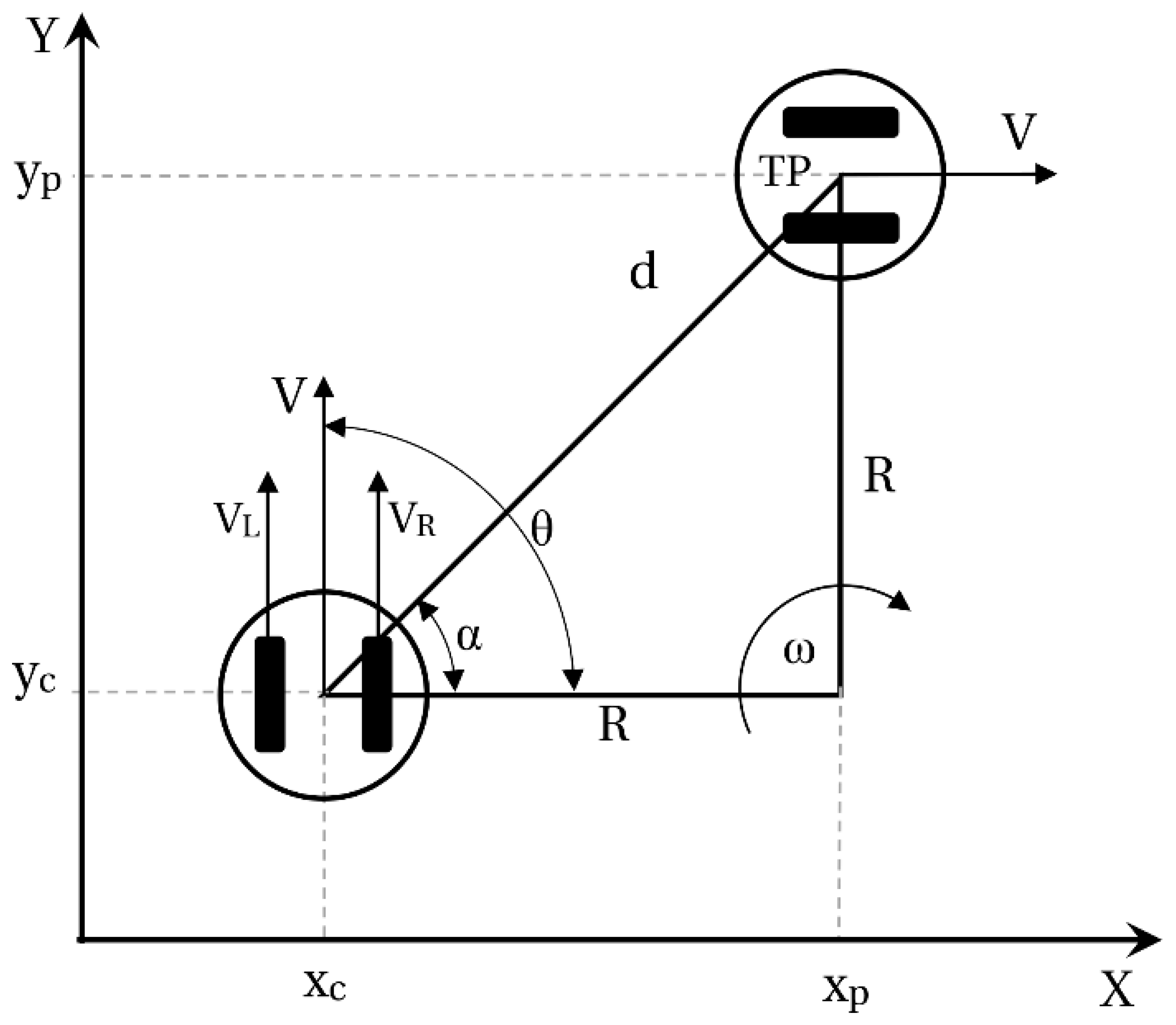
The problem of controlling the position of a mobile robot consists of maneuvering the vehicle from its current position, $C\left(x_c,y_c\right)$, to a target point, TP $=\left(x_p, y_p\right)$, manipulating the angular velocity, $\omega$, and the linear velocity, $v$, of the mobile robot. To achieve this maneuver, we define the distance $d$ (Equation (2)), the angle $\alpha$ (Equation (3)) between the robot and the TP and the angular error $O_c$ (Equation (4)) from the scheme in Figure 2. A graphical scheme of the control of the position of a differential robot is presented in this figure.

$$d=\sqrt{{\left(y_p-y_c\right)}^2+{\left(x_p-x_c\right)}^2}$$

(2)

$$\alpha ={\tan }^{-1}\left(\frac{y_p-y_c}{x_p-x_c}\right)$$

(3)

$$O_c={\tan }^{-1}\left(\frac{\sin \left(\alpha -\theta \right)}{\cos \left(\alpha -\theta \right)}\right)$$

(4)

The angular error $O_c$ lies between the $\pi$ and $-\pi$ values and is equivalent to the subtraction between $\alpha$ and $\theta$ within that interval. To get the robot to reach the TP, we seek to reduce the distance and the angular error between $\alpha$ and $\theta$.

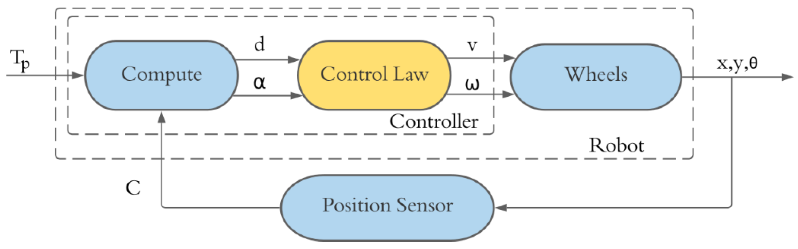
By using control algorithms, such as the Villela algorithm and the IPC algorithm, a set of rules to be followed for the control law can be defined. Thus, Figure 3 shows the block diagram of the implementation of the control law for the control algorithms; in this work, the Villela and IPC algorithms are used, which have their control laws defined by Equations (5) and (6) for Villela and by Equations (7) and (8) for IPC.

$$v=\{\begin{array}{cc}{v}_{max}& if \left|d\right|>k_r\\ d\left(\frac{v_{max}}{k_r}\right)& if \left|d\right|\le k_r\end{array}$$

(5)

$$\mathsf{\omega }={\mathsf{\omega }}_{max}\sin \left(\alpha -\theta \right)$$

(6)

where $v_{max}$ and ${\mathsf{\omega }}_{max}$ are the maximum values of the lineal and angular velocities, respectively, and $k_r$ is a radio of a docking area of the TP.

$$v=\min \left\{k_v p\left(O_c\right) d, v_{max}\right\}$$

(7)

$$\mathsf{\omega }=k_p\sin \left(O_c\right)+k_i{{\displaystyle \int }}_0^t{O}_c dt$$

(8)

where $k_v$, and $k_i$ are the tuning parameters of the IPC algorithm obtained empirically and $p\left(O_c\right)=1-\left|O_c\right|/\pi$, for $O_c\in \left[-\pi ,\pi \right]$ [4].

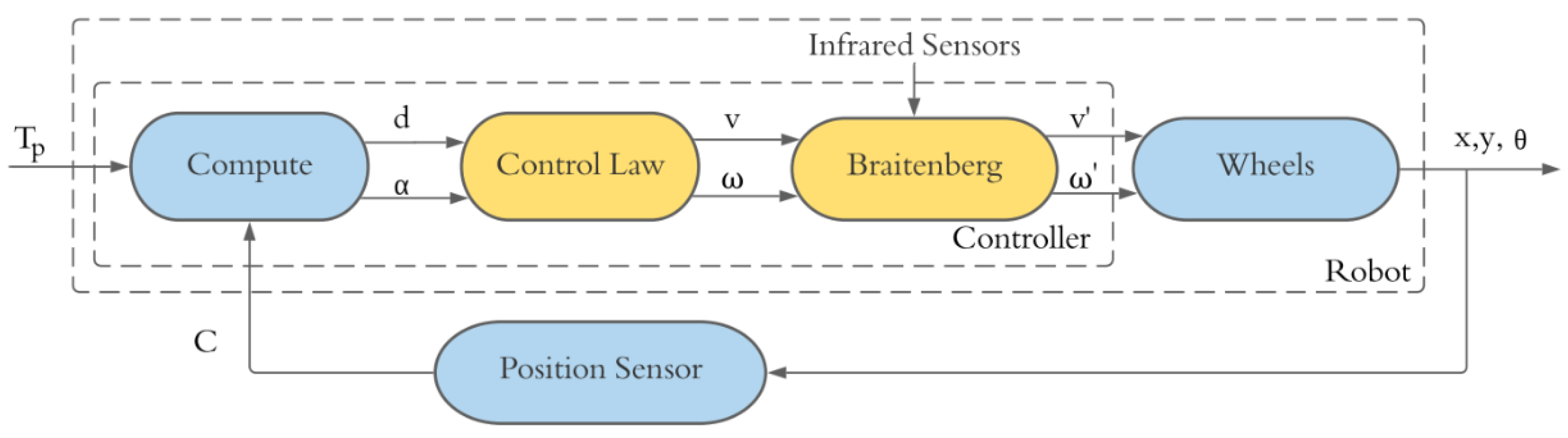
Once the problem of position control has been solved, we can add obstacles to the trajectory of the robot and avoid them. This can be archived by adding a new block of obstacle avoidance, such as the Braitenberg algorithm [46]. This method builds a weighted matrix that converts the measurements of obstacle sensors (eight infrared sensors for the Khepera) into new lienal and angular velocities, just as how its shown in Figure 4. For more details, see [46].

4. Simulated Environment and Mobile Robot

To perform the experiments, a simulated environment was created to perform the position control of the mobile robot Khepera IV. The basic elements used for the construction of environments compatible with the Gym library, the simulation program and the robot are presented below, which are part of the simulated platform and are used to make the comparison between the control and deep reinforcement learning.

4.1. Robot Khepera IV

The robot used in this work is a simulation of the mobile robot Khepera IV of the K-Team company (Figure 5); it has two main wheels that share a common axis and are controlled by independent motors, and it can have one or more rotating wheels that serve as support and prevent it from tipping over. It has a compact and modular design, making it perfect for research and education in various fields, such as autonomous navigation, artificial intelligence, multiagent systems and automatic control. Despite its small size, this robot has a wide range of sensors. It has an array of eight infrared sensors to detect obstacles, four more sensors to avoid falls or follow lines, five ultrasonic sensors to detect long-range objects, an accelerometer, a gyroscope and a color camera. It has two DC motors of very high quality, efficiency and precision. It also has a powerful Linux kernel with WiFi and Bluetooth for communication between devices and a large battery with an autonomy of approximately 7 h.

4.2. CoppeliaSim

To create the environment, CoppeliaSim is used—a robotics 3D simulation platform that is widely used in contexts such as robotics education, human–robot interaction and reinforcement learning. Its architecture is based on a distributed control of objects or robots, which can be controlled individually through a script, a plugin, an ROS node or a remote API client. This design makes CoppeliaSim very versatile and ideal for multirobot applications. Controllers can be written in C/C++, Python, Java, Lua, MATLAB or Octave. CoppeliaSim comes with sensors, actuators and robot models included by default, with which you can virtually recreate an environment and interact with it in real time. For the simulation, we used the 3D model of the Khepera robot corresponding to the one provided by the KH4VREP library [47]. The model assumes that the mobile robot has a rigid structure and wheels that do not deform or slide.

To control the position of the Khepera robot, the remote API in Python will be used, which makes communication between CoppeliaSim and external applications possible. This allows for the programming of the reinforcement learning algorithms, which allows for a bidirectional transmission of information [48]. To perform the position control, CoppeliaSim communicates with Keras-RL2 [49], which allows for the implementation of state-of-the-art deep reinforcement learning algorithms in Python. Please check the implementation of the environments and the connection with Keras RL in the following repository: https://github.com/Fco-Quiroga/gym-kheperaposition (accessed on 12 July 2022).

4.3. Environments

To generate an interface that converts the CoppeliaSim simulation to an environment compatible with RL agents and control algorithms, the OpenAI Gym library is used. Gym provides a simple definition of RL environments, formalized as partially observable Markov decision processes (POMDPs) [40]. Figure 6 is a diagram of the communication that happens in the environments and shows the flow of information between the algorithm or agent, the gym environment, the API and, finally, the CoppeliaSim program.

The environments correspond to a simulation of a platform in the CoppeliaSim program, where there is a simulated mobile robot Khepera IV and a red hemisphere (see Figure 7) located on the surface of the platform (in some cases, obstacles are present). The objective is to drive the robot from its current position to a predefined target point (the red sphere). Each episode ends when the TP is reached, when the maximum number of steps allowed per episode is exceeded, when the robot leaves the maximum allowed area (4 square meters) or when the robot collides with an obstacle, if any. At the beginning of a new episode, the position of the TP and that of the robot are randomly changed, as is the orientation of the robot.

The reward function is observed in Equation (9), As the robot draws close to the TP, the reward increases until it becomes zero. In addition, when using the environment to train an agent, collisions are allowed, but they are penalized, adding a negative factor $\left(r_{collision}=-10\right)$ to the reward; in this way, the robot learns to not collide with obstacles. Additionally, when the robot reaches the TP, a positive reward is delivered $\left(r_{arrival}=100\right)$, rewarding the robot for reaching its goal. The values of $r_{collision}$ and $r_{arrival}$ were determined empirically to minimize the training time of the RL agents and maximize their performance in the experiments.

$$\mathrm{reward}=\{\begin{array}{c}\begin{array}{cc}{r}_{arrival}& if the robot reaches the \mathrm{TP}\end{array}\\ \begin{array}{cc}{r}_{collision}-\left(d^2\right)& if the robot collides\end{array}\\ \begin{array}{cc}-\left(d^2\right)& in another case\end{array}\end{array}$$

(9)

Two environments were created with different action spaces, depending on the agent to be used. In the case of DQN, there is a discrete action space of size 3: turn left, go straight or turn right, which correspond to the minimum set of instructions that allow for free movement in the environment. For DDPG, the set of actions is continuous so that the linear and angular velocities of the robot can be manipulated, these two being the action space. Continuous actions are normalized to obtain better agent behavior, but in the environment, they are mapped to the allowed values of linear and angular velocity.

The observation space for these environments is presented in

Table 1. Observation space.

Number	Observation	Minimum	Maximum
0	$\mathrm{Distance} \mathrm{to} \mathrm{TP} \left(d\right)$	0	2.82
1	$\mathrm{Angular} \mathrm{error} \left(O_c\right)$	$-\pi$	$\pi$
2	Linear velocity in previous step	0	0.05
3	Angular velocity in previous step	$-\pi /4$	$\pi /4$
4 to 12	Distance measurements from eight infrared sensors	0	1

. Table 1 shows that the values used correspond to the distance to the TP ($d$), which varies between 0 and 2.82 m (minimum and maximum distance between the robot and the TP); the angular error $\left(O_c\right)$ between the orientation of the robot and the TP, with values between $-\pi$ and $\pi$; the linear and angular velocity for the previous step; and an arrangement with the measurements of the eight sensors that the Kephera IV robot has. The sensors take measurements from 0 to 20 cm, but the data are normalized between 0 and 1. All these values can be obtained from the simulation or calculated by requesting information from the API, such as the position of the robot and the TP, which helps to calculate the distance to the TP and the angular error. In a real case, the absolute position and orientation of the robot can be obtained by using an Indoor Positioning System (IPS) [50]. Note that the action space depends only on the agent or algorithm to be used; instead, the observation space depends on the environment and its physical constraints.

5. Experiments and Results

Next, the experiments to control the position of a mobile robot and obstacle avoidance are explained. In addition, how the training of each of the agents was performed and an analysis of the obtained results are presented.

5.1. Experiments

5.1.1. Khepera Robot Position Control

The first experiment corresponds to the problem of controlling the position of the mobile robot. The two deep reinforcement learning agents, DQN and DDPG, were used and compared with the two control algorithms: Villela and IPC. Figure 7a corresponds to an image of the simulated environment for the position control used in this experiment.

5.1.2. Position Control with Obstacles

The second experiment corresponds to the problem of controlling the position of the mobile robot with disturbances (obstacles). The Kephera robot must reach its target point, crossing obstacles without collision. For this experiment, the RL algorithms (DDPG and DQN) and control algorithms, (IPC and Villela with the Braitenberg obstacle avoidance algorithm [51]) are used. Figure 7b shows the environment of the obstacle position control used in this experiment.

5.2. Training of RL Agents

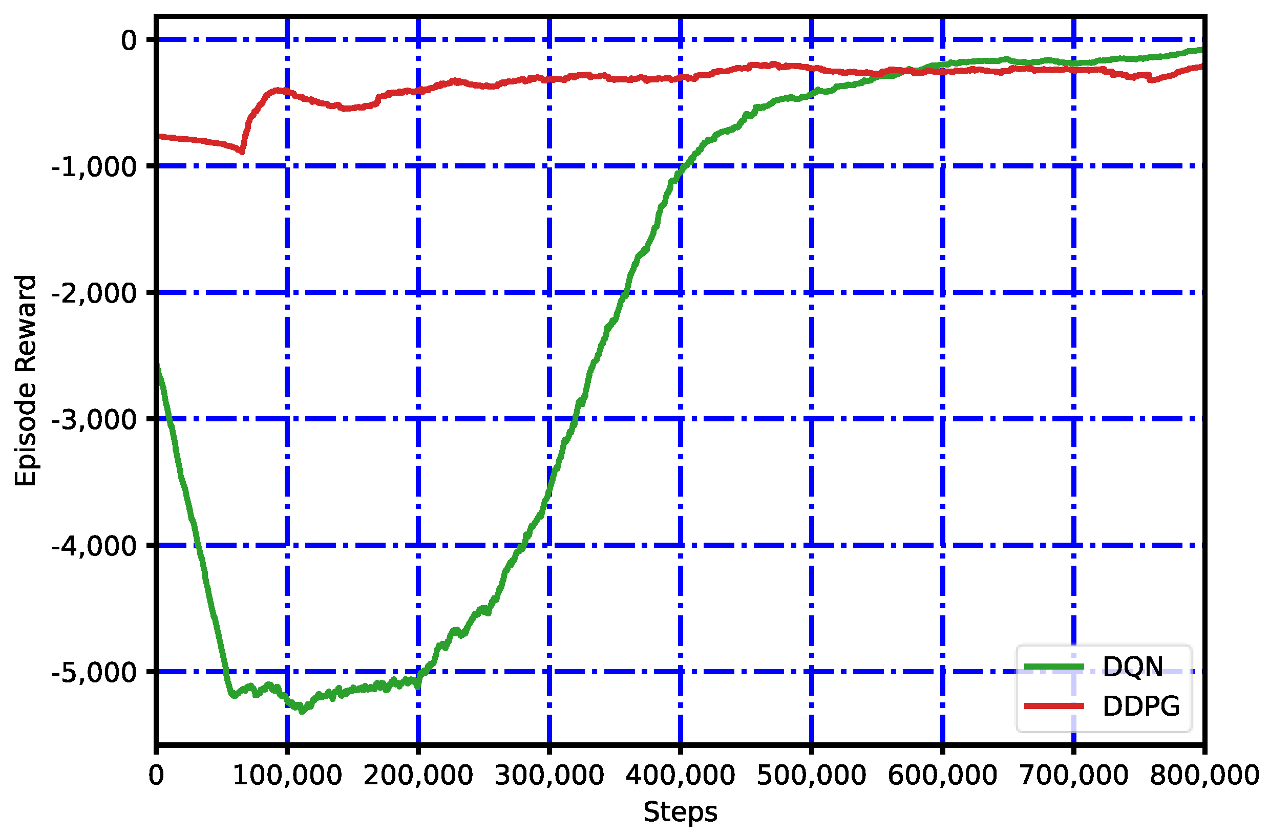
The RL agents were trained by a million steps, which took approximately 8.6 h in the case of DQN and 11.4 h for DDPG. Figure 8 shows the reward per episode of the DDPG and DQN agents, the gradual increase in the reward and how the agent learns from the environment. Notably, DQN’s learning is “slower” than that of DDPG because DDPG achieves greater rewards from the 100,000 steps, unlike DQN, improving from 550,000 steps, but this effect should be mostly due to the technique used to address the exploitation–exploration trade-off effect, which, in the case of DQN, is Epsilon Greedy. Both algorithms can learn properly in their training.

5.3. Results

After training, the agents are tested by assigning them positions with new targets, maintaining the same initial conditions for the two algorithms. For these effects, the best weights obtained from the DQN and DDPG training were chosen, with which a better action policy can be obtained in the environment. The first environment consists of using only one target point, while the second environment uses multiple target points to analyze the position control with and without obstacles.

5.3.1. One Target Point

For the case without obstacles, the initial position of the robot is represented by a black circle at (−0.4, 0), while the target point is represented by a red circle at position (0.8, 0). The orientation of the robot is indicated by a black arrow with a value of −178° (the values extracted from the experiments are presented in [52]).

Figure 9 shows a graph of the trajectory followed by the robot for each algorithm. Please observe how the RL, Villela and IPC agents manage to fulfill the task, reaching the desired target. Figure 10 shows the robot trajectory for the RL agents and the control algorithms for the environment with obstacles. A blue circle symbolizes the presence of an obstacle in the path of the robot to the target point. All the algorithms can reach the target, dodging the obstacle by using their sensors. In addition, the control algorithms result in a wider curve than the RL agents, maintaining a greater distance from the obstacle.

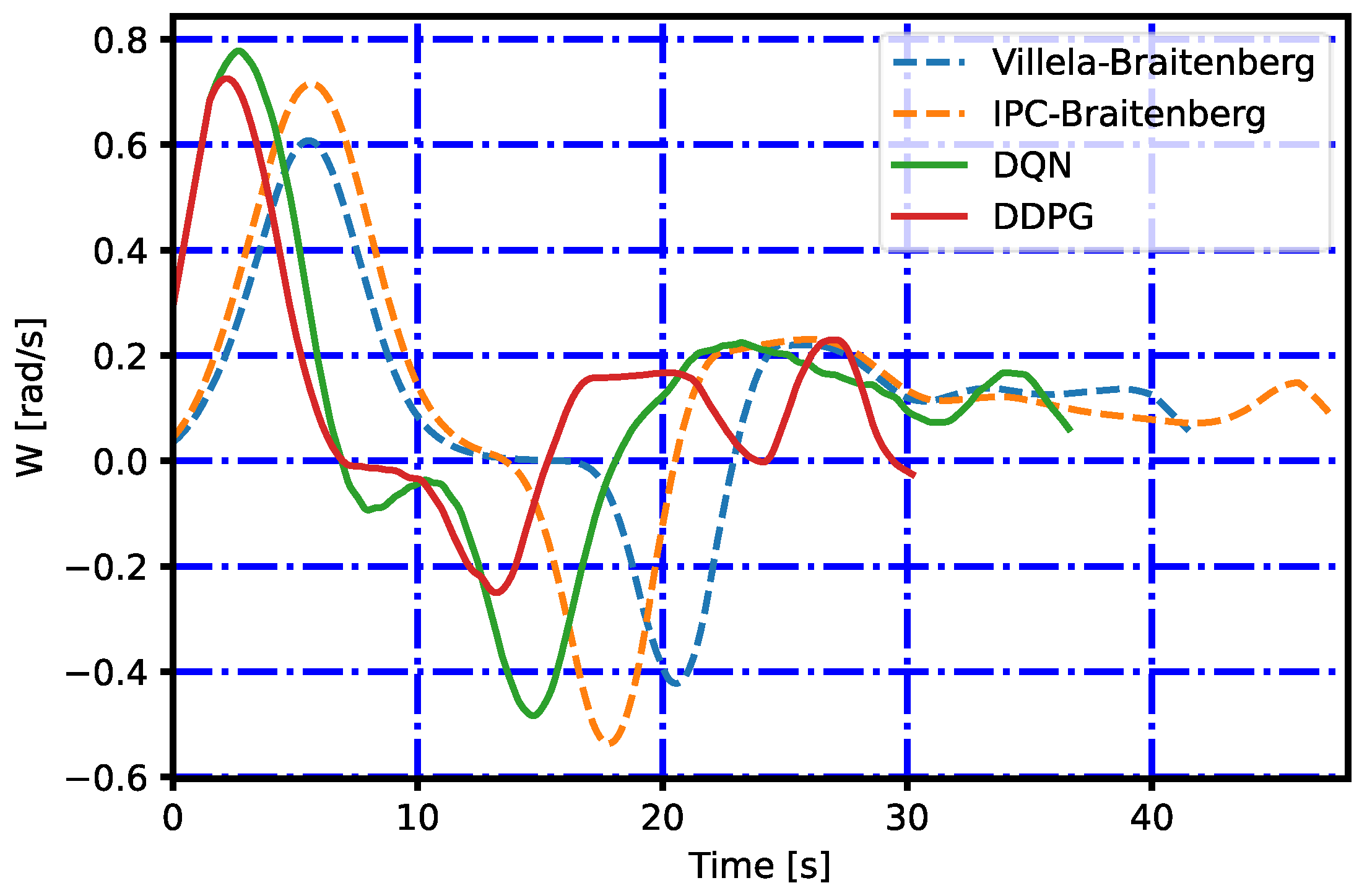
To analyze how the angular velocity of the robot varies, Figure 11 and Figure 12 are presented for the environment without and with obstacles, respectively. Figure 11 shows that the control algorithms have similar behaviors, taking approximately 10 s to rotate and orient themselves to the target point. The RL agents are oriented to the target faster, but they continue to maneuver the robot throughout the experiment. These algorithms reach the target point first. For the case with obstacles, Figure 12 shows how the algorithms in the first instance maneuver to orient themselves toward the target and then again to avoid the obstacle. The control algorithms show a slower behavior than the RL agents.

To perform an analysis of the arrival times at the target point of each algorithm,

Table 2. Time to reach the target point for the experiment without an obstacle.

Algorithm	Times (s)
Villela	33.95
IPC	30.40
DQN	28.75
DDPG	27.40

and

Table 3. Time to reach the target point for the experiment with an obstacle.

Algorithm	Times (s)
Villela–Braitenberg	41.50
IPC–Braitenberg	47.55
DQN	36.45
DDPG	30.20

are presented, where the best values obtained are marked in bold. In Table 2, the arrival times of the different algorithms at the target point can be observed. Notice how DDPG has the best time (27.4 s), followed by DQN, IPC and, finally, Villela (33.95 s). For the experiment with obstacles, in Table 3, the DDPG reaches the target point very quickly (30.2 s), avoiding the obstacle in a better way than DQN, Villela and IPC Braitenberg. In both experiments, the RL agents perform this task the fastest. All of the algorithms tested in this work are capable of maneuvering the robot by manipulating its linear and angular velocities. The difference in the time it takes for the robot to reach the TP is mainly due to the trajectory but also to the linear velocity that the Khepera robot has. RL agents learn to set the linear velocity to the maximum allowed value almost all of the time, in contrast to control methods such as IPC, which reduce the linear velocity when the angular velocity is non-zero, i.e., when the robot is turning.

Finally, a comparative table of the control and RL algorithms is made using the performance indices in both environments (with and without obstacles). The indices to be evaluated correspond to the integral of the absolute magnitude (IAE), the integral of the square of the error (ISE), the integral of time multiplied by the absolute error (ITAE) and the integral of time multiplied by the squared error (ITSE). From

Table 4. Performance indices for the environment without obstacles.

Index	Villela	IPC	DQN	DDPG
ISE	30.94	22.62	19.53	18.04
IAE	28.92	23.42	21.08	19.66
ITSE	301.92	195.92	158.02	131.99
ITAE	351.39	254.32	213.51	187.5

, it is observed that the RL agents obtain better results for all the indices, with DDPG having the best performance.

Table 5. Performance indices for the environment with obstacles.

Index	Villela–Braitenberg	IPC–Braitenberg	DQN	DDPG
ISE	33.64	27.96	22.79	19.07
IAE	33.45	32.20	26.05	21.32
ITSE	386.75	343.27	233.22	154.48
ITAE	498.41	533.28	346.31	226.06

shows that the DDPG agent again obtains better results for all the indices, followed by DQN, IPC–Braitenberg and Villela–Braitenberg. To summarize the improvement of the RL agents, they have a faster response at the beginning of the experiment, decreasing their distance to the target in the first steps of time, adjusting much better than the control algorithm and reducing the error. DQN and DDPG obtain the best results.

5.3.2. Multiple Target Points

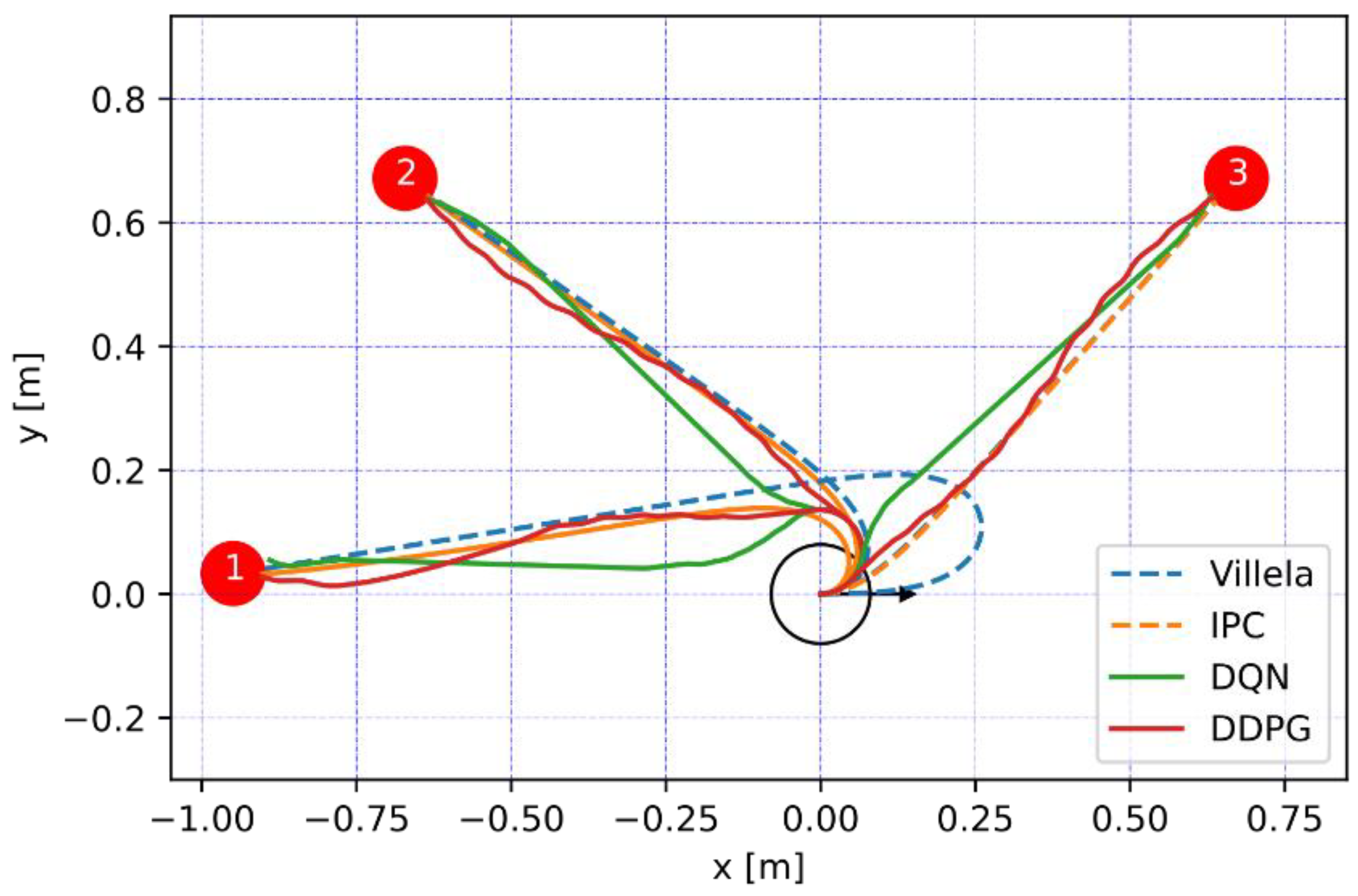
Next, it will be analyzed what happens with the control of the robot’s position in front of multiple target points—specifically, three target points for environments without and with obstacles. Target points 1, 2 and 3 are located 0.95 m from the robot, with an angular difference from the robot’s orientation of 178°, 135° and 45°, respectively.

The objective of the multiple targets experiment is to evaluate the robustness of the proposed algorithms with respect to changes produced by the robot orientation versus the target point position. This experiment allows us to evaluate the control algorithms, since they exhibit low performance when the orientations of the target point and the robot have a high angular error—for example, when $O_c\approx 180°$.

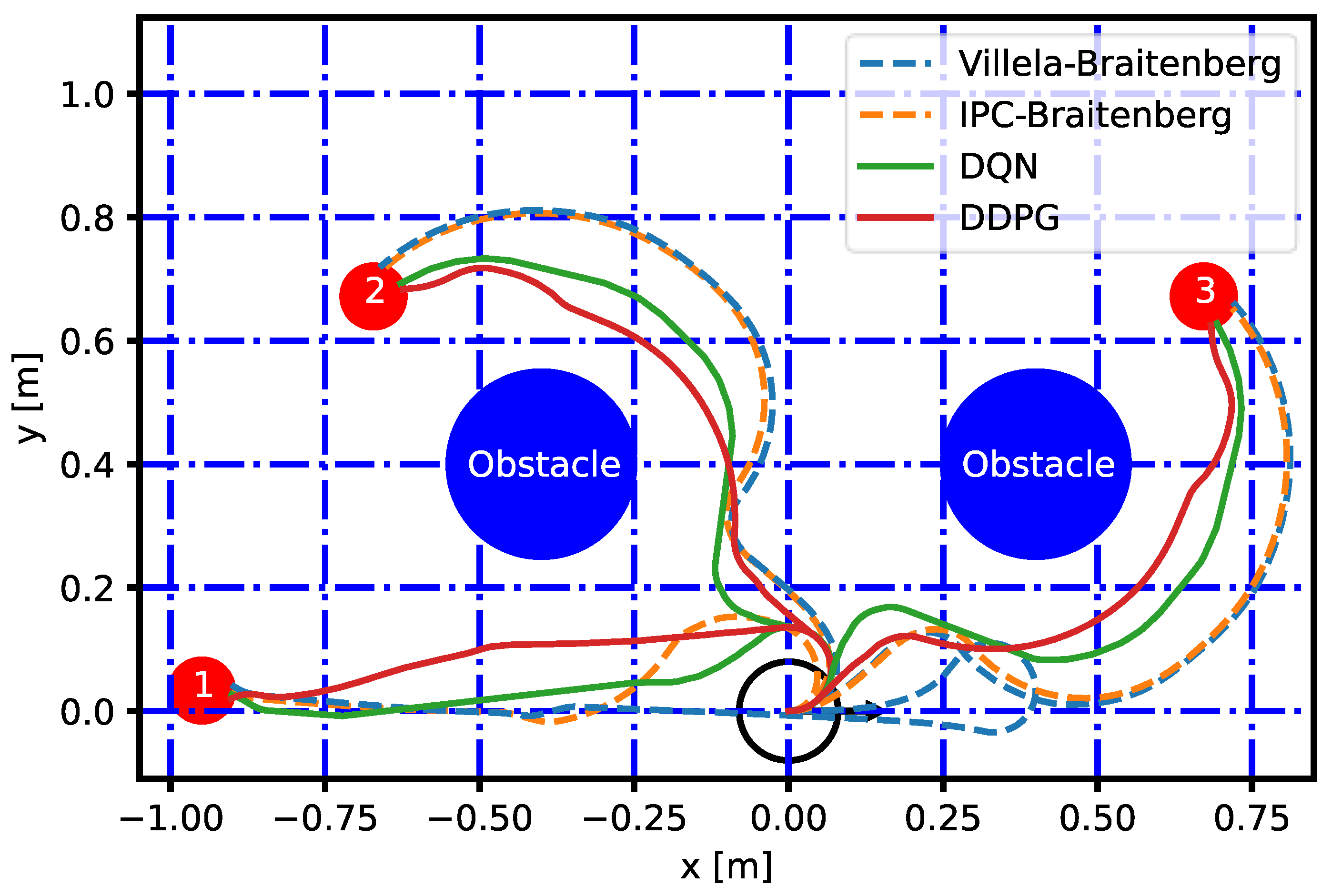
Figure 13 shows a graph with the trajectories made by the robot for the environment without obstacles. All of the algorithms manage to reach their target points; however, DDPG and DQN have trajectories that react earlier, reaching the target before Villela and IPC, which adjust more to reach the target point. Figure 14 shows the trajectory of the robot in an environment with obstacles. The DDPG agent has the shortest trajectory, allowing it to reach the target point faster, followed by DQN. In contrast, the agents controlled by the Villela and IPC methods move away from obstacles, maintaining a distance of approximately 20 cm, which corresponds to the maximum distance of its sensor’s measurement.

To make a better comparison of the times used in the experiments,

Table 6. Arrival time for the three target points for the experiment without obstacles.

Algorithm	TP 1 s	TP 2 s	TP 3 s	Mean Time (s)
Villela	30.45	20.80	18.25	23.17
IPC	25.85	20.70	18.25	21.60
DQN	22.50	20.65	18.35	20.50
DDPG	22.60	20.55	18.30	20.48

shows the time taken to reach the targets for the experiment without obstacles. Note how DDPG and DQN obtain the lowest times on average compared to the control algorithms; however, in some cases, the control algorithms obtain a performance comparable to that of the RL agents.

Table 7. Arrival time for the three target points for the experiment with obstacles.

Algorithm	TP 1 s	TP 2 s	TP 3 s	Mean Time (s)
Villela–Braitenberg	36.45	28.85	27.95	31.08
IPC–Braitenberg	27.90	50.65	50.05	42.87
DQN	23.00	25.65	24.75	24.47
DDPG	22.50	23.40	22.15	22.68

shows the time taken to reach the target points in the case of the obstacle experiment. The excellent performance of DDPG is observed, reaching its TPs in 22.68 s, on average.

To finish the analysis,

Table 8. Average performance indices (three target points) in the experiment without obstacles.

Index	Villela	IPC	DQN	DDPG
ISE	14.52	14.44	11.43	11.30
IAE	11.68	90.5	8.08	7.95
ITSE	132.47	99.72	83.67	82.27
ITAE	89.16	58.29	45.86	44.61

and

Table 9. Average performance indices (three target points) in the experiment with obstacles.

Index	Villela–Braitenberg	IPC–Braitenberg	DQN	DDPG
ISE	20.72	19.82	13.82	12.60
IAE	17.42	13.01	9.61	8.77
ITSE	251.91	276.84	123.23	102.00
ITAE	182.20	131.94	67.21	54.95

were added, showing the average performance indices for each algorithm in the experiments without and with obstacles, respectively. From Table 8, it is observed how the RL algorithms once again present very favorable results, indicating that the control of the position of a mobile robot can be performed efficiently with RL algorithms. Table 9 shows that DDPG obtains very low metrics, it being the algorithm to choose to perform this type of task.

6. Discussion

The results obtained from the experiments show how the DDPG and DQN algorithms exhibit adequate decision making in reaching the targets in environments with and without obstacles. This finding is reflected through an analysis of metrics and variables such as trajectory, angular velocity and time. When comparing the results with the control algorithms, it is shown that DDPG and DQN obtain shorter arrival times at the destination point, and it is possible to dominate environments with and without obstacles.

Reinforcement learning agents can obtain a route point by point in real time and only need information about the environment, the robot position and the position of the target point. The position of the obstacle can be random since, in the training process, the position of the robot was changed at every episode. In this way, the agent did not learn the position of the obstacles but learned only to rely on the sensor’s data, so when a new obstacle appears, the robot will be able to avoid it.

7. Conclusions

This article presents the use of reinforcement learning algorithms and two control algorithms to control the position of the mobile robot Kephera IV in a simulated environment. The work shows the effectiveness of RL algorithms in comparison with control algorithms for the task of position control in environments with and without obstacles.

The use of RL agents has a substantial advantage in controlling the position of robots because they learn from experience and can improve decision making compared to control algorithms. The results obtained show how the DDPG and DQN agents manage to obtain the shortest times taken to reach the target point in environments with and without obstacles; however, the time required to learn all the robot interactions is high compared to that of the control algorithms.

In future work, we will consider two important tasks: first, to make a comparison with other types of algorithms, such as adaptive neural networks [53], PPO (proximal policy optimization) [54], Muesli [55], neuroevolution [56] and adaptive NN dynamic surface controllers [57,58]; second, to perform the transfer of learning from the simulation to the real world [18,19,20], which will allow us to validate our theoretical and simulated results in real environments, analyze whether reinforced learning agents can operate with more complex tasks, corroborate decision making in the face of different obstacles (more complex shapes and layouts) and analyze the reaction times used to start the motors of the robot, among other things.

References

- Klancar, G.; Zdesar, A.; Blazic, S.; Skrjanc, I. Introduction to Mobile Robotics, in Wheeled Mobile Robotics: From Funda-Mentals towards Autonomous Systems; Butterworth-Heinemann: Oxford, UK, 2017; pp. 1–11. [Google Scholar]
- Fabregas, E.; Farias, G.; Peralta, E.; Vargas, H.; Dormido, S. Teaching control in mobile robotics with V-REP and a Khepera IV library. In Proceedings of the 2016 IEEE Conference on Control Applications, Buenos Aires, Argentina, 19–22 September 2016; pp. 821–826. [Google Scholar] [CrossRef]
- Villela, V.J.; Parkin, R.; Parra, M.; Dorador, J.M.; Dorador, J.M.; Guadarrama, M.J. A wheeled mobile robot with obstacle avoidance capability. Ing. Mecánica Tecnología Desarro. 2004, 1, 159–166. [Google Scholar]
- Fabregas, E.; Farias, G.; Aranda-Escolastico, E.; Garcia, G.; Chaos, D.; Dormido-Canto, S.; Bencomo, S.D. Simulation and Experimental Results of a New Control Strategy For Point Stabilization of Nonholonomic Mobile Robots. IEEE Trans. Ind. Electron. 2019, 67, 6679–6687. [Google Scholar] [CrossRef]
- Alajlan, A.M.; Almasri, M.M.; Elleithy, K.M. Multi-sensor based collision avoidance algorithm for mobile robot. In Proceedings of the 2015 Long Island Systems, Applications and Technology, Farmingdale, NY, USA, 1 May 2015; pp. 1–6. [Google Scholar] [CrossRef]
- Almasri, M.M.; Alajlan, A.M.; Elleithy, K.M. Trajectory Planning and Collision Avoidance Algorithm for Mobile Robotics System. IEEE Sens. J. 2016, 16, 5021–5028. [Google Scholar] [CrossRef]
- Almasri, M.; Elleithy, K.; Alajlan, A. Sensor Fusion Based Model for Collision Free Mobile Robot Navigation. Sensors 2015, 16, 24. [Google Scholar] [CrossRef] [Green Version]
- Wang, H.; Bai, W.; Liu, P.X. Finite-time adaptive fault-tolerant control for nonlinear systems with multiple faults. IEEE/CAA J. Autom. Sin. 2019, 6, 1417–1427. [Google Scholar] [CrossRef]
- Chen, M.; Wang, H.; Liu, X. Adaptive Fuzzy Practical Fixed-Time Tracking Control of Nonlinear Systems. IEEE Trans. Fuzzy Syst. 2019, 29, 664–673. [Google Scholar] [CrossRef]
- Peng, S.; Shi, W. Adaptive Fuzzy Output Feedback Control of a Nonholonomic Wheeled Mobile Robot. IEEE Access 2018, 6, 43414–43424. [Google Scholar] [CrossRef]
- Ludvi, E.A.; Bellemare, M.G.; Pearson, K.G. A Primer on Reinforcement Learning in the Brain: Psychological, Computational, and Neural Perspectives, Computational Neuroscience for Advancing Artificial Intelligence: Models, Methods and Applications; Medical Information Science: Hershey, NY, USA, 2011. [Google Scholar]
- Silver, D.; Huang, A.; Maddison, C.J.; Guez, A.; Sifre, L.; van den Driessche, G.; Schrittwieser, J.; Antonoglou, I.; Panneershelvam, V.; Lanctot, M.; et al. Mastering the game of Go with deep neural networks and tree search. Nature 2016, 529, 484–489. [Google Scholar] [CrossRef]
- Vinyals, O.; Babuschkin, I.; Czarnecki, W.M.; Mathieu, M.; Dudzik, A.; Chung, J.; Choi, D.H.; Powell, R.; Ewalds, T.; Georgiev, P.; et al. Grandmaster level in StarCraft II using multi-agent reinforcement learning. Nature 2019, 575, 350–354. [Google Scholar] [CrossRef]
- OpenAI Five. OpenAI Five Defeats Dota 2 World Champions. Available online: https://openai.com/blog/openai-five-defeats-dota-2-world-champions/, (accessed on 12 July 2022).
- Schrittwieser, J.; Antonoglou, I.; Hubert, T.; Simonyan, K.; Sifre, L.; Schmitt, S.; Guez, A.; Lockhart, E.; Hassabis, D.; Graepel, T.; et al. Mastering Atari, Go, chess and shogi by planning with a learned model. Nature 2020, 588, 604–609. [Google Scholar] [CrossRef]
- Andrychowicz, O.M.; Baker, B.; Chociej, M.; Józefowicz, R.; McGrew, B.; Pachocki, J.; Petron, A.; Plappert, M.; Powell, G.; Ray, A.; et al. Learning dexterous in-hand manipulation. Int. J. Robot. Res. 2019, 39, 3–20. [Google Scholar] [CrossRef] [Green Version]
- Chebotar, Y.; Handa, A.; Makoviychuk, V.; Macklin, M.; Issac, J.; Ratliff, N.; Fox, D. Closing the Sim-to-Real Loop: Adapting Simulation Randomization with Real World Experience. arXiv 2019, arXiv:1810.05687v4. [Google Scholar] [CrossRef] [Green Version]
- Zhao, W.; Queralta, J.P.; Qingqing, L.; Westerlund, T. Towards Closing the Sim-to-Real Gap in Collaborative Multi-Robot Deep Reinforcement Learning. arXiv 2020, arXiv:2008.07875v1. [Google Scholar] [CrossRef]
- Hu, H.; Zhang, K.; Tan, A.H.; Ruan, M.; Agia, C.G.; Nejat, G. A Sim-to-Real Pipeline for Deep Reinforcement Learning for Autonomous Robot Navigation in Cluttered Rough Terrain. IEEE Robot. Autom. Lett. 2021, 6, 6569–6576. [Google Scholar] [CrossRef]
- Niu, H.; Ji, Z.; Arvin, F.; Lennox, B.; Yin, H.; Carrasco, J. Accelerated Sim-to-Real Deep Reinforcement Learning: Learning Collision Avoidance from Human Playerar. arXiv 2021, arXiv:2102.10711v2. [Google Scholar] [CrossRef]
- Smart, W.; Kaelbling, L.P. Effective reinforcement learning for mobile robots. In Proceedings of the 2002 IEEE International Conference on Robotics and Automation, Washington, DC, USA, 11–15 May 2002; Volume 4, pp. 3404–3410. [Google Scholar] [CrossRef]
- Surmann, H.; Jestel, C.; Marchel, R.; Musberg, F.; Elhadj, H.; Ardani, M. Deep Reinforcement learning for real autonomous mobile robot navigation in indoor environments. arXiv 2020, arXiv:2005.13857v1. [Google Scholar]
- Farias, G.; Garcia, G.; Montenegro, G.; Fabregas, E.; Dormido-Canto, S.; Dormido, S. Reinforcement Learning for Position Control Problem of a Mobile Robot. IEEE Access 2020, 8, 152941–152951. [Google Scholar] [CrossRef]
- Watkins, C.J.; Dayan, P. Q-learning. Mach. Learn. 1992, 8, 279–292, Thecnical Note. [Google Scholar]
- Ganapathy, V.; Soh, C.Y.; Lui, W.L.D. Utilization of Webots and Khepera II as a platform for Neural Q-Learning controllers. In Proceedings of the 2009 IEEE Symposium on Industrial Electronics & Applications, Kuala Lumpur, Malaysia, 4–6 October 2009; Volume 2, pp. 783–788. [Google Scholar] [CrossRef]
- Huang, B.-Q.; Cao, G.-Y.; Guo, M. Reinforcement Learning Neural Network to the Problem of Autonomous Mobile Robot Obstacle Avoidance. In Proceedings of the 2005 International Conference on Machine Learning and Cybernetics, Guangzhou, China, 18–21 August 2005; Volume 1, pp. 85–89. [Google Scholar] [CrossRef]
- Hagen, S.T.; Kröse, B. Neural Q-learning. Neural Comput. Appl. 2003, 12, 81–88. [Google Scholar] [CrossRef]
- Kulathunga, G. A Reinforcement Learning based Path Planning Approach in 3D Environment. arXiv 2022, arXiv:2105.10342v2. [Google Scholar] [CrossRef]
- Wang, Y.; Fang, Y.; Lou, P.; Yan, J.; Liu, N. Deep Reinforcement Learning based Path Planning for Mobile Robot in Unknown Environment. J. Phys. Conf. Ser. 2020, 1576, 012009. [Google Scholar] [CrossRef]
- Wang, B.; Liu, Z.; Li, Q.; Prorok, A. Mobile Robot Path Planning in Dynamic Environments Through Globally Guided Reinforcement Learning. IEEE Robot. Autom. Lett. 2020, 5, 6932–6939. [Google Scholar] [CrossRef]
- Duguleana, M.; Mogan, G. Neural networks based reinforcement learning for mobile robots obstacle avoidance. Expert Syst. Appl. 2016, 62, 104–115. [Google Scholar] [CrossRef]
- Tai, L.; Paolo, G.; Liu, M. Virtual-to-real deep reinforcement learning: Continuous control of mobile robots for mapless navigation. In Proceedings of the 2017 IEEE/RSJ International Conference on Intelligent Robots and Systems (IROS), Vancouver, BC, Canada, 24–28 September 2017; pp. 31–36. [Google Scholar]
- Lillicrap, T.; Hunt, J.; Pritzel, A.; Hees, N.; Erez, T.; Tassa, Y.; Silver, D.; Wierstra, D. Continuous Control with Deep Reinforcement Learning; International Conference on Learning Representation: London, UK, 2016. [Google Scholar]
- Alyasin, A.; Abbas, E.I.; Hasan, S.D. An Efficient Optimal Path Finding for Mobile Robot Based on Dijkstra Method. In Proceedings of the 2019 4th Scientific International Conference Najaf (SICN), Al-Najef, Iraq, 29–30 April 2019; pp. 11–14. [Google Scholar] [CrossRef]
- Yufka, A.; Parlaktuna, O. Performance Comparison of BUG Algorithms for Mobile Robots. In Proceedings of the 5th International Advanced Technologies Symposium, Karabuk, Turkey, 7–9 October 2020. [Google Scholar] [CrossRef]
- ElHalawany, B.M.; Abdel-Kader, H.M.; TagEldeen, A.; Elsayed, A.E.; Nossair, Z.B. Modified A* algorithm for safer mobile robot navigation. In Proceedings of the 2013 5th International Conference on Modelling, Identification and Control (ICMIC), Cairo, Egypt, 31 August–2 September 2013; pp. 74–78. [Google Scholar]
- Team, K.; Tharin, J.; Lambercy, F.; Caroon, T. Khepera IV User Manual; K-Team: Vallorbe, Switzerland, 2019. [Google Scholar]
- Mnih, V.; Kavukcuoglu, K.; Silver, D.; Graves, A.; Antonoglou, I.; Wierstra, D.; Riedmiller, M. Playing Atari with Deep Reinforcement Learning, Deepmind. arXiv 2013, arXiv:1312.5602, 1–9. [Google Scholar]
- Rohmer, E.; Singh, S.; Freese, M. CoppeliaSim (formely V-Rep): A Verstile and Scalable Robot Simulation Framework. In Proceedings of the 2013 IEEE/RSJ International Conference on Intelligent Robots and Systems, Tokyo, Japan, 3–7 November 2013. [Google Scholar]
- Brockman, G.; Cheung, V.; Patterson, L.; Schneider, J.; Schulman, J.; Tang, J.; Zaremba, W. OpenAI Gym. arXiv 2016, arXiv:1606.01540v1. [Google Scholar]
- Puterman, M.L. Model formulation. In Markov Decision Processes: Discrete Stochastic Dynamic Programming, 1st ed.; John Wiley & Sons: Hoboken, NJ, USA, 2005; pp. 17–32. [Google Scholar]
- Sutton, R.S.; Barto, A.G. Reinforcement Learning: An Introduction, 2nd ed.; The MIT Press: Cambridge, MA, USA, 2017. [Google Scholar]
- Berger-Tal, O.; Nathan, J.; Meron, E.; Saltz, D. The Exploration-Exploitation Dilemma: A Multidisciplinary Framework. PLoS ONE 2014, 9, e95693. [Google Scholar] [CrossRef] [Green Version]
- Mnih, V.; Kavukcuoglu, K.; Silver, D.; Rusu, A.A.; Veness, J.; Bellemare, M.G.; Graves, A.; Riedmiller, M.; Fidjeland, A.K.; Ostrovski, G.; et al. Human-level control through deep reinforcement learning. Nature 2015, 518, 529–533. [Google Scholar] [CrossRef]
- Zagoraiou, M.; Antognini, A.B. Optimal designs for parameter estimation of the Ornstein-Uhlenbeck process. Appl. Stoch. Model. Bus. Ind. 2008, 25, 583–600. [Google Scholar] [CrossRef]
- Yang, X.; Patel, R.V.; Moallem, M. A Fuzzy–Braitenberg Navigation Strategy for Differential Drive Mobile Robots. J. Intell. Robot. Syst. 2006, 47, 101–124. [Google Scholar] [CrossRef]
- Farias, G.; Fabregas, E.; Peralta, E.; Torres, E.; Dormido, S. A Khepera IV library for robotic control education using V-REP. IFAC-PapersOnLine 2017, 50, 9150–9155. [Google Scholar] [CrossRef]
- Remote API. Coppelia Robotics. Available online: https://www.coppeliarobotics.com/helpFiles/en/remoteApiOverview.htm, (accessed on 12 July 2022).
- McNally, T. Keras RL2. 2019. Available online: https://github.com/wau/keras-rl2; (accessed on 12 July 2022).
- Farias, G.; Fabregas, E.; Torres, E.; Bricas, G.; Dormido-Canto, S.; Dormido, S. A Distributed Vision-Based Navigation System for Khepera IV Mobile Robots. Sensors 2020, 20, 5409. [Google Scholar] [CrossRef] [PubMed]
- Yang, X.; Patel, R.V.; Moallem, M. A Fuzzy-Braitenberg Navigation Strategy for Differential Drive Mobile Robots. IFAC Proc. Vol. 2004, 37, 97–102. [Google Scholar] [CrossRef]
- Farias, G.; Fabregas, E.; Peralta, E.; Vargas, H.; Dormido-Canto, S.; Dormido, S. Development of an Easy-to-Use Multi-Agent Platform for Teaching Mobile Robotics. IEEE Access 2019, 7, 55885–55897. [Google Scholar] [CrossRef]
- Li, S.; Ding, L.; Gao, H.; Chen, C.; Liu, Z.; Deng, Z. Adaptive neural network tracking control-based reinforcement learning for wheeled mobile robots with skidding and slipping. Neurocomputing 2018, 283, 20–30. [Google Scholar] [CrossRef]
- Schulman, J.; Wolski, F.; Dhariwal, P.; Radford, A.; Klimov, O. Proximal Policy Optimization Algorithms. arXiv 2017, arXiv:1707.06347v2. [Google Scholar]
- Hessel, M.; Danihelka, I.; Viola, F.; Guez, A.; Schmitt, S.; Sifre, L.; Weber, T.; Silver, D.; Hasselt, H. Muesli: Combining Improvements in Policy Optimization. arXiv 2021, arXiv:2104.06159v1. [Google Scholar]
- Petroski, F.; Madhavan, V.; Conti, E.; Lehman, J.; Stanley, K.O.; Clune, J. Deep Neuroevolution: Genetic Algorithms Are a Competitive Alternative for Training Deep Neural Networks for Reinforcement Learning. arXiv 2018, arXiv:1712.06567. [Google Scholar]
- Niu, B.; Li, H.; Qin, T.; Karimi, H.R. Adaptive NN Dynamic Surface Controller Design for Nonlinear Pure-Feedback Switched Systems With Time-Delays and Quantized Input. IEEE Trans. Syst. Man Cybern. Syst. 2017, 48, 1676–1688. [Google Scholar] [CrossRef]
- Niu, B.; Li, H.; Zhang, Z.; Li, J.; Hayat, T.; Alsaadi, F.E. Adaptive Neural-Network-Based Dynamic Surface Control for Stochastic Interconnected Nonlinear Nonstrict-Feedback Systems With Dead Zone. IEEE Trans. Syst. Man Cybern. Syst. 2018, 49, 1386–1398. [Google Scholar] [CrossRef]
Figure 1.
RL scheme and interactions [42].
Figure 2.
Position control of a differential robot [4].
Figure 3.
Diagram of the position control problem of a control algorithm [4].
Figure 4.
Diagram of the position control problem with the Braitenberg algorithm [46].
Figure 5.
Mobile Robot Khepera IV: (a) real robot [37], (b) simulated robot.
Figure 6.
Communication diagram.
Figure 7.
Environments for position control: (a) without obstacles; (b) with obstacles.
Figure 8.
Reward per episode during the agent training.
Figure 9.
Graph of the trajectory of the experiment without obstacles.
Figure 10.
Graph of the trajectory of the experiment with obstacles.
Figure 11.
Angular velocity of the experiment without obstacles.
Figure 12.
Angular velocity of the experiment with obstacles.
Figure 13.
Graph of the trajectory for the three target points in the environment without obstacles.
Figure 14.
Graph of the trajectory for the three target points in the environment with obstacles.