
An Intelligent DOA Estimation Error Calibration Method Based on Transfer Learning

1
College of Electronic Engineering, National University of Defense Technology, Hefei 230031, China
2
Xi’an Satellite Control Center, Xi’an 710043, China
*
Author to whom correspondence should be addressed.
Appl. Sci. 2022, 12(15), 7636; https://0-doi-org.brum.beds.ac.uk/10.3390/app12157636
Submission received: 16 June 2022
/
Revised: 25 July 2022
/
Accepted: 26 July 2022
/
Published: 28 July 2022
(This article belongs to the Special Issue Future Information & Communication Engineering 2022)
Abstract
:Affected by various error factors in the actual environment, the accuracy of the direction of arrival (DOA) estimation algorithm will greatly decrease during an application. To address this issue, in this paper, we propose an intelligent DOA estimation error calibration method based on transfer learning, which learns error knowledge from a small number of actual signal samples and improves the DOA estimation accuracy in the real application. We constructed a deep convolutional neural network (CNN)-based intelligent DOA estimation model to learn the mapping between the input signals and their azimuths. We generated a large number of ideal simulation signal samples to train the CNN model and used it as the pretrained model. Then, we fine-tuned the CNN model with a small number of actual signal samples collected in the actual environment. We demonstrate the effectiveness of the proposed method through simulation experiments. The experimental results indicate that the proposed method can effectively improve the accuracy of DOA estimation in the actual environment.
1. Introduction
DOA estimation is an important branch of array signal processing, and has been widely used in military and civilian application fields such as radar, sonar, communications, seismic exploration, radio astronomy, and other fields. Many classical DOA estimation algorithms have been proposed in recent decades, such as subspace-based algorithms represented by the multiple signal classification (MUSIC) [1], sparse reconstruction based algorithms [2], etc. However, these algorithms can only perform with high DOA estimation accuracy under ideal conditions. In practical applications, the performance of the above algorithms suffers due to various error factors such as the amplitude and phase error of the array channel, the mutual coupling error between array elements and the array element position error.
Many error calibration methods have been proposed to calibrate various error factors in the real environment. These error calibration methods can be divided into two categories. One is the active calibration method, wherein the error perturbation parameters are estimated offline by setting up an auxiliary signal source with precisely known direction in space [3,4,5]. The other is a self-calibration method based on some optimization functions for the joint estimation of the spatial orientation of the signal source and the perturbation error parameters of the array [6,7,8,9,10]. All these calibration methods deal with the actual signal and try to eliminate various error factors in the signal. The goal is to make the actual signal consistent with the ideal simulation signal, thus improving the DOA estimation accuracy of the algorithm. However, due to the complexity of the actual environment, the above error calibration methods cannot cope with the effects of multiple error factors. With the development of artificial intelligence, DOA estimation error calibration algorithms based on machine learning are studied [11,12,13,14,15,16]. In recent years, there have been some deep learning-based methods in DOA estimation. However, the application of deep learning in DOA estimation is not yet widespread [17]. Recently, works have mainly used deep neural networks (DNN) [16,18,19] and convolutional neural networks (CNN) [20,21,22,23] to construct DOA estimation models. In existing deep learning-based methods, researchers have focused on how to learn the complex mapping between signals and their azimuths and how to enhance the DOA estimation performance based on DNNs and CNNs.
However, the existing deep learning-based methods mostly work under ideal conditions. Due to the various error factors in the actual environment, the accuracy of DOA estimation in the practical applications of these methods will be greatly reduced. In order to make DNN-based DOA estimation models work well in the actual environment, a large number of actual signal samples need to be collected, however, this is very difficult. In addition, when the environment changes, a large number of samples need to be re-collected and the model needs to be re-trained. Therefore, it is a great challenge to quickly calibrate errors and to make the DNN-based models efficiently applicable in the actual environment.
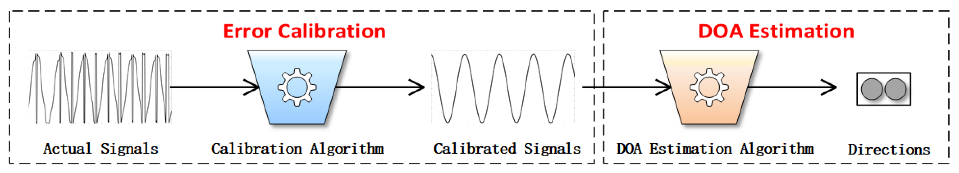
To address the above issue, in this paper, we propose an intelligent DOA estimation error calibration method based on transfer learning. Transfer learning [24,25,26,27] can adaptively update the trained model according to the new samples, and transfer the model to new tasks. The idea of transfer learning suits the task of DOA estimation. The large number of ideal signal samples generated by computer simulation can be used to train a DNN-based DOA estimation model to learn the mapping between signals and their azimuths. The small number of actual signal samples collected from the actual environment can be used to fine-tune the model based on transfer learning. The original DOA estimation capability of the model is retained while the model can learn new error knowledge during transfer learning. As such, only a small number of actual signal samples need to be collected, and the model can calibrate the errors and be quickly applied in the actual environment. When the environment changes, the model can continuously learn the error knowledge in new environments by learning from a small number of new actual signal samples. Specifically, the proposed method is implemented as follows. First, we construct an intelligent DOA estimation model based on CNN. Second, we generate a large number of ideal simulation signal samples to train the CNN model. Third, we use a small number of actual signal samples collected in the actual environment to fine tune the CNN model. The proposed method has the following advantages: (i) It is a one-stage error calibration method that is different from the traditional two-stage methods. Figure 1 shows the traditional two-stage error calibration methods. These use calibration algorithms to process the input actual signals. The calibrated signals are input to the DOA estimation algorithm to predict the directions of signals. The error calibration and the DOA estimation are two separate modules and the error calibration module can only consider a single or partial error factor. Figure 2 shows the proposed method. The DOA estimation model trained on ideal signal samples is fine-tuned with actual signal samples. It implements both error calibration and DOA estimation on the same model. All the error factors in the environment are taken into consideration. (ii) This requires only a small number of actual samples to fine-tune the model, saving a lot of time and manpower. (iii) It is environmentally adaptable. In a new environment, only a small number of actual signal samples need to be collected. After approximately a few dozen epochs of fine-tuning, the model is ready for practical application.
The main contributions of this paper are as follows:
- We propose an intelligent DOA estimation error calibration method based on transfer learning, which learns error knowledge of the actual environment from a small number of signal samples and improves the DOA estimation accuracy in practical application.
- We generate a large number of ideal simulation signal samples to train an intelligent DOA estimation model constructed based on CNN. Then, we fine tune the model with a small number of actual signal samples collected in the actual environment. Before and after transfer learning, the model’s tasks are the same, and the working environment is transferred from the ideal condition to the actual environment.
- We experimentally show that transfer learning can effectively improve the DOA estimation accuracy in practical application. We further discuss the impact of different fine-tuning approaches (freezing different network layers) and different numbers of actual samples used for fine-tuning. The experimental results indicate that the intelligent DOA estimation model performs better when freezing the first convolutional layer. The more actual signal samples are used for fine-tuning, the better the model performs.
2. Background
2.1. Signal Model
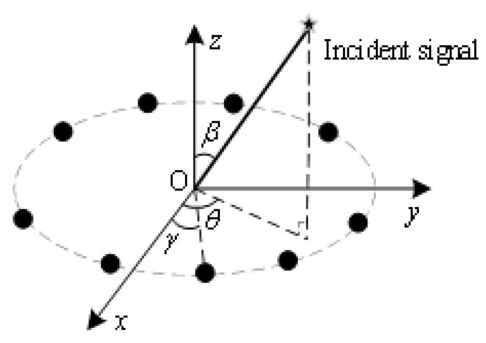
Figure 3 shows a uniform circle array of radius r consisting of M omnidirectional elements. Assuming that p far-field signals are incident on a uniform circular array, the received signal of the l-th element at moment t is:
where is the receiver noise of the l-th antenna since the signals incident on the antenna array elements is assumed to have some noise associated with them. is the propagation time delay, calculated as follows:
where are the angular positions of the antenna array elements which can be calculated as . Equation (1) can be written in a matrix form:
where , , are given by:
where is an dimension array snapshot vector, is dimension array noise vector, is dimension space signal vector, and A is dimension array steering vector matrix.
Among them, the steering vector is:
The fast Fourier transform algorithm is used to extract the phase difference of the input array signal as an input to the intelligent DOA estimation model. The phase difference between the i-th element and the j-th element of a uniform circular array is represented by . The phase difference of the signal of array elements can be expressed as the phase difference square array, as shown in Equation (9).
Figure 3.
Schematic diagram of M-element uniform circular array.

2.2. The Error of Signals
Equation (3) is the expression of the array signal received under ideal conditions. In the actual environment, the signal of the antenna array changes a lot due to various error factors. Considering various error factors, the vector form of the signal can be written as follows:
where , C is the mutual coupling error between array elements, is amplitude, and the phase error of the array channel and is the array element position error. Due to various errors in the actual environment, there is a great difference between actual signal samples and ideal simulation signal samples. When considering a five-element uniform circular array with a radius of m, the frequency is 163~167 MHz, the angle step is 5°, and the frequency interval is 1 MHz. Figure 4a shows the phase difference between the two array elements of 300 simulation signal samples generated by a computer under ideal conditions. Figure 4b shows the phase difference between two array elements of 300 actual signal samples collected in the actual environment.
It can be seen that the phase difference in the ideal condition is very different from the phase difference in the actual environment due to various error factors in the actual environment. Because the signal in the actual environment is affected by many complex error factors, such as mutual coupling error, amplitude and phase error of array channel, and array element position error, these errors make the DOA estimation performance of the model sharply decline in the actual environment. A deep neural network (DNN) can learn the complex mapping relationship between signals and their azimuths. However, it is difficult to collect a large number of actual signal samples for training. Therefore, we propose the error calibration method based on transfer learning to make the DNN-based DOA estimation models work well in the actual environment. The large number of ideal signal samples generated by computer simulation are used to train a DNN-based model and learn the mapping between signals and their azimuths. The small number of actual signal samples are used to fine-tune the model based on transfer learning and learn the complex error factors. As such, the model is transferred from the ideal condition to the actual environment, and hence error calibration is achieved.
3. Models and Methods
Figure 5 shows the overall framework of the proposed method, where a large number of ideal simulation signal samples are generated as source domain data to train an ideal intelligent DOA estimation model. The source task is DOA estimation under ideal conditions. We collect a small number of actual signal samples as target domain data . Under the effect of the knowledge transfer of and , the model is fine-tuned. The target task is DOA estimation in the actual environment.
The covariance matrix of the phase difference between elements can be regarded as a direction image. It not only contains all information about the direction of an incident signal, but also eliminates some noise and interference [28]. Therefore, we use CNN to construct the DOA estimation model. The CNN can continuously extract the features of data in layers. The multi-layer linear and nonlinear processing units of CNN are superimposed in a hierarchical manner, which provides the ability to learn complex representations at different levels of abstraction. Thus, it is good at learning the complex characteristics of array signals.
3.1. The DOA Estimation Model Based on CNN
Figure 6 shows the structure of the intelligent DOA estimation model based on CNN, which consists of five convolutional layers and one fully connected layer.
The input of the first convolutional layer is the phase difference characteristic matrix.
The feature of the l-th convolutional layer is expressed as , where the feature is composed of several feature maps . is the number of convolutional kernels as well as the number of output feature maps in the l-th convolutional layer. The calculation of is as follows:
where, is the convolutional kernel of the l-th layer, ⊗ represents the convolutional operation, represents the bias, and uses the nonlinear function as the activation function. The calculation is as follows:
The features of each layer can be calculated as follows:
The output feature of the last convolutional layer is flattened into a one-dimensional vector and input into the fully connected layer, which is computed as follows:
where is the flatten operation, and W and b, respectively, represent the connection weight and offset of the fully connected layer. is adopted as the activation function. The calculation is as follows:
The parameter set of the intelligent DOA estimation model based on CNN can be expressed as follows:
Among them, k and b are the parameters of convolutional layers, W and are the parameters of the fully connected layer.
3.2. Error Calibration Method Based on Transfer Learning
After training a CNN-based intelligent DOA estimation model with a large number of ideal simulation signal samples, the CNN model is used as a pretrained model. A small number of actual signal samples are used to fine-tune the pretrained model.
Figure 7 shows the error calibration method based on transfer learning. The first t convolutional layers are frozen, and the weight is not updated. The weight of the -th to the last convolutional layer and the weight of the fully connected layer is updated. That is to keep the parameters unchanged.
The parameters are updated.
The gradient of the convolutional layers is calculated as follows:
where is the input sum of the j-th neuron of the l-th convolutional layer, is the weight of the convolutional layer, which represents the connection weight between the i-th neuron of the l-th layer and the j-th neuron of the -th layer, and is the error of convolutional layers. When updating the weights, the gradient descent algorithm is used to calculate the gradient g for a batch of samples.
where m is the number of samples for a batch, and is the sample error. Adaptive time estimation (Adam) is used to optimize the gradient. The gradient of the first-order moment vector s and the second-order moment vector r over time t is calculated as follows:
where and are the exponential decay rates of moment estimation. The calibrated first-order moment vector deviation and second-order moment vector deviation are as follows:
is the learning rate, is a small constant—generally —and the weights are updated as follows:
Figure 7.
Proposed transfer learning method.

When the model has trained to convergence again, the training is stopped. The Algorithm 1 is as follows.
| Algorithm 1: Error calibration method based on transfer learning |
| Input: A large number of ideal simulation signal samples , A small number of actual samples . |
| Output: Fine-tuning trained DOA estimation model |
Process:
|
4. Simulation and Result Analysis
- Experiment environment. The ideal array signal sample is a five-element uniform circular array signal with a frequency range of 100 MHz–200 MHz, signal-to-noise ratio set to 0–25 db, angle range of 0–360°, and interval of 1°. The actual signal sample is a five-element uniform circular array signal collected in the actual environment, with a frequency range of 150 MHz–200 MHz, an angle range of 0–360°, and an interval of 5°.Collection of actual signals. We use a circular array of five-channel ultrashortwave correlation interferometer direction finding equipment to collect the actual signal samples, and the data obtained is the phase difference data of the actual signal.The receiving antenna array of the ultrashort wave direction-finding equipment we used to collect actual signal samples is five-element uniform circular array. The antenna array is divided into upper and lower layers. The upper layer is used to receive ultrashort wave spatial signal source and the working frequency band is vertical polarization 800~3000 MHz. The lower layer is used to collect a short-wave spatial signal source and the working frequency band is vertical polarization 30~800 MHz. We use the five-element uniform circular array of the lower layer to collect the actual signal samples. Figure 8 shows the positions of the five elements, the five antenna elements are evenly distributed on the circumference with radius m, and the included angle between adjacent elements is 72°. The frequency range is 151~200 MHz, the azimuth range is 0~360°, the angle step is 5°, and the frequency interval is 1 MHz. A total of 3600 samples of actual signal samples were collected, and some of them are shown in Table 1, where represents the phase difference between the array element i and array element j.Table 1. The phase difference between the elements of some actual signals.
Frequency
(MHz)Azimuth
(°)151 −81.397 −131.6 −0.24426 131.66 81.587 0 151 −71.317 −135.07 −12.096 127.76 90.726 5 151 −60.364 −137.2 −24.359 122.38 99.546 10 151 −49.47 −138.45 −35.756 116.07 107.61 15 Frequency
(MHz)Azimuth
(°)151 147 −131.85 131.41 −146.75 0.19037 0 151 153.61 −147.17 115.66 −141.51 19.409 5 151 162.43 −161.56 98.021 −138.07 39.182 10 151 172.08 −174.21 80.31 −136.32 58.141 15 Figure 8. The ultrashort wave direction-finding antenna array.![Applsci 12 07636 g008]() Generation of simulation signals. We generate the simulation signal samples of a five-element uniform circular array with radius m by computer. The frequency range is 100~200 MHz, the azimuth range is 0~360°, the angle step is 1°, and the frequency interval is 0.5 MHz, and the signal-to-noise ratio is 0~25 db. A total of 72,000 samples of actual signal samples were generated.
Generation of simulation signals. We generate the simulation signal samples of a five-element uniform circular array with radius m by computer. The frequency range is 100~200 MHz, the azimuth range is 0~360°, the angle step is 1°, and the frequency interval is 0.5 MHz, and the signal-to-noise ratio is 0~25 db. A total of 72,000 samples of actual signal samples were generated. - Evaluation metrics. There are four evaluation metrics for the intelligent DOA estimation model: average absolute angle error (MAE), root mean square angle error (RMSE), maximum absolute angle error (MAXE), and the ratio of absolute angle error less than 1° (Ratio-1).The MAE is calculated as follows:The RMSE is calculated as follows:The MAXE is calculated as follows:The Ratio-1 is calculated as follows:Among them, is the test angle, is the actual angle, N is the number of test samples, and is the operation of counting quantity.
- Datasets. Training Dataset : 72,000 ideal simulation signal samples are generated under ideal conditions, with a frequency range of 100 MHz–200 MHz. Training Dataset : 1800 actual signal samples are collected in the actual environment, with a frequency range of 150 MHz–200 MHz. Test Dataset D: 1800 actual signal samples, which are different with , with a frequency range of 150 MHz–200 MHz. Angular values of all signal samples are replaced by sine and cosine values, which are the labels.


4.1. Model Structure and Parameters
The intelligent DOA estimation model is constructed based on CNN. The structure and parameters of the model are shown in Table 2.
Before transfer learning, the batch size is set to 360, and the learning rate is set to 0.001. We use the early stop strategy for training. When the validation error does not decrease for five epochs, the training will be stopped. When transfer learning, we fine tune the model with a smaller learning rate of 0.0001, other parameters remain unchanged.
4.2. Experimental Results
We use the training dataset to train the intelligent DOA estimation model to convergence, and test it on the test dataset D. Then, set a smaller learning rate, use the training dataset to fine-tune the model and update the parameters of all convolutional layers and the fully connected layer. When the model has trained to convergence again, test it on the test set D. In Section 4.2.1, we show the test performance on the four evaluation metrics of the model before and after transfer learning. In Section 4.2.2, we show how close the predicted angles are to the actual angles before and after transfer learning. In Section 4.2.3, we show the test angle error distribution before and after transfer learning.
4.2.1. Test Performance on MAE, RMSE, MAXE, and Ratio-1
Test results before and after transfer learning on the four evaluation metrics are shown in Table 3.
We can observe from the result in Table 3 that the performance of the model after transfer learning has been greatly improved. The average angle error MAE drops from 13.77° to 0.716°, the root mean square angle error RMSE decreased from 34.72° to 0.912°, the maximum angular error MAXE decreased from 179.827° to 3.775°, and the ratio of absolute error less than 1° Ratio-1 increased from 0.043 to 0.737. What can be inferred from the test result can be found below:
- Transfer learning enables the model to learn the error knowledge in the actual environment with a small number of actual signal samples.
- The error calibration method we proposed based on transfer learning can effectively improve the DOA estimation performance of the model in practical application.
4.2.2. Test Angle
Figure 9a shows the test angles and the actual angles for each signal sample in a test dataset D before transfer learning. The blue circles are labels, and the red lines are the angles of the model prediction. Figure 9b shows the test angles and the actual angles after transfer learning. We can observe from Figure 9 that after transfer learning, the model’s test accuracy is greatly improved. Before transfer learning, there is a large difference between the predicted azimuths and the actual azimuths, especially when the frequency increases. After transfer learning, the predicted azimuths are very close to the actual azimuths.
4.2.3. Test Error Distribution
We make statistics on the test angle error of the actual samples and draw the distribution diagram, as shown in Figure 10. Figure 10a shows the test angle error distribution of the model before transfer learning, and Figure 10b shows the error distribution after transfer learning.
We can observe from Figure 10 that before transfer learning, the test angle errors are mostly distributed between −50° and 50°, and there are some large angle errors below −100° or over 100°. After transfer learning, the error is mainly distributed between −1° and 1°, and the maximum angle error of the model is reduced between −5° and 5°. We can infer from the test result that our error calibration method based on transfer learning greatly reduces the overall DOA estimation error.
5. Further Analysis
5.1. Freeze Different Layers
A common method in transfer learning is to freeze some layers, fix their parameters, and fine-tuning updates the parameters of other layers. In this experiment, we, respectively, froze the first 0, 1, 2, 3, 4, and 5 convolutional layers. Freezing the first 0 convolutional layers will open all network layers for fine-tuning. Freezing the first five convolutional layers will freeze all convolutional layers, and fine-tuning updates the parameters of the fully connected layer. Freeze different network layers and use the same training dataset so that fine-tuning may train the model. Test results on the four evaluation metrics are as shown in Table 4.
We can observe from Table 4 that when different network layers are frozen, the test results of the model are different. When the first convolutional layer is frozen and the next four convolutional layers and the fully connected layer are fine-tuning trained, the test result is better than other freezing approaches. Although the maximum angle error is 4.02°, which is higher than the minimum value of 3.775°, this may be due to the large individual error caused by the randomness of the samples. When all the convolutional layers are frozen and only the fully connected layer is fine-tuning trained, the performance of the model is much lower.
From the above test results, we can draw inferences as follows:
- The convolutional layer is the main feature extraction module, and the fully connected layer is the classification module. When all convolutional layers are frozen, the test results of the model are poor, while when some convolutional layers are opened, the test results of the model are significantly improved. This is because the feature extraction module is needed to be fine-tuned when training samples are transferred from the ideal condition to the actual condition.
- In CNN, different convolutional layers extract different features from the input data. The first few convolutional layers extract the common features (bottom features) of the data, and the last few extract the individual features (high-level features), and the transition from the common features to the individual features occurs on some middle layers.
5.2. Different Numbers of Actual Samples
Another important factor is the number of actual signal samples. In this experiment, we randomly selected 360, 720, 1080, 1440, and 1800 actual samples to fine-tune the model and freeze the first convolutional layer. Because a small number of actual signal samples are used to fine tune the model during transfer learning, the selection of a small number of samples has a large impact on the model performance. Therefore, we repeat the experiment five times with different numbers of randomly selected samples, and the average of the five sets of experimental results is taken as the final experimental result. The performance of the model on the test dataset D on four evaluation metrics is shown in Table 5.
We can observe from Table 5 that MAE, RMSE, and MAXE keep decreasing overall and Ratio-1 keeps increasing as the actual sample number increases. The maximum angular error MAXE refers to the error of the one with the largest angular error among all the test samples, which is further influenced by some individual samples. Therefore, it is reasonable for MAXE to have some volatility. When all 1800 samples in the training set are used, the performance of the model is relatively the greatest, with an MAE of 0.678°, RMSE of 0.86°, MAXE of 4.02°, and ratio-1 of 0.766. It can be inferred that the larger the sample size in the target domain, the more knowledge the model learns, and the better the performance of the model in the target task.
6. Conclusions
In this paper, we propose an intelligent DOA estimation error calibration method based on transfer learning, which learns error knowledge from a small number of samples. We generate a large number of ideal simulation signal samples to train the model constructed based on CNN. The CNN model learns the mapping between input signals and their azimuths. Then, we use a small number of actual signal samples collected in the actual environment to fine tune the model. During the fine-tuning process, the model learns the knowledge of various error factors. Through experimental comparison and analysis, this method can effectively improve the DOA estimation accuracy in practical applications. It is of great significance for intelligent DOA estimation from an ideal simulation to practical engineering application. Despite the preliminary results in this paper, however, fine-tuning is a relatively simple approach of transfer learning. In future work, we will investigate more reasonable transfer learning approaches to make the model better learn the error knowledge in the actual environment.
Author Contributions
Conceptualization, M.Z. and W.Z.; methodology, M.Z. and C.W.; software, C.W. and W.Z.; validation, M.Z. and Y.S.; formal analysis, M.Z.; investigation, M.Z. and C.W.; resources, W.Z.; data curation, W.Z.; writing—original draft preparation M.Z. and C.W.; writing—review and editing M.Z. and W.Z.; visualization, Y.S.; supervision, M.Z. All authors have read and agreed to the published version of the manuscript.
Funding
This research was funded by the National Natural Science Foundation of China, grant number 61971473.
Institutional Review Board Statement
Not applicable.
Informed Consent Statement
Not applicable.
Data Availability Statement
Not applicable.
Acknowledgments
This work is supported by the National Natural Science Foundation of China 61971473 and Anhui Provincial Natural Science Foundation 1908085QF291.
Conflicts of Interest
The authors declare no conflict of interest.
References
- Schmidt, R. Multiple emitter location and signal parameter estimation. IEEE Trans. Antennas Propag. 1986, 34, 276–280. [Google Scholar] [CrossRef] [Green Version]
- Bilik, I. Spatial compressive sensing for direction-of-arrival estimation of multiple sources using dynamic sensor arrays. IEEE Trans. Aerosp. Electron. Syst. 2011, 47, 1754–1769. [Google Scholar] [CrossRef]
- Tian, Y.; Wang, Y.; Shi, B. Gain-phase errors calibration of nested array for underdetermined direction of arrival estimation. AEU-Int. J. Electron. Commun. 2019, 108, 87–90. [Google Scholar] [CrossRef]
- Wang, D.; Wu, Y. A novel array errors active calibration algorithm. Acta Electonica Sin. 2010, 38, 517. [Google Scholar]
- Sellone, F.; Serra, A. A Novel Online Mutual Coupling Compensation Algorithm for Uniform and Linear Arrays. IEEE Trans. Signal Process. 2007, 55, 560–573. [Google Scholar] [CrossRef]
- Zhang, J.; Chen, H.; Huang, W.; Liu, W. Self-calibration of mutual coupling for non-uniform cross-array. Circuits Syst. Signal Process. 2019, 38, 1137–1156. [Google Scholar] [CrossRef]
- Zhang, X.; He, Z.; Zhang, X.; Yang, Y. DOA and phase error estimation for a partly calibrated array with arbitrary geometry. IEEE Trans. Aerosp. Electron. Syst. 2019, 56, 497–511. [Google Scholar] [CrossRef]
- Qin, L.; Li, C.; Du, Y.; Li, B. DoA estimation and mutual coupling calibration algorithm for array in plasma environment. IEEE Trans. Plasma Sci. 2020, 48, 2075–2082. [Google Scholar] [CrossRef]
- Deli, C.; Gong, Z.; Huamin, T.; Huanzhang, L. Approach for wideband direction-of-arrival estimation in the presence of array model errors. J. Syst. Eng. Electron. 2009, 20, 69–75. [Google Scholar]
- Wahlberg, B.; Ottersten, B.; Viberg, M. Robust signal parameter estimation in the presence of array perturbations. In Proceedings of the ICASSP 91: 1991 International Conference on Acoustics, Speech, and Signal Processing, Toronto, ON, Canada, 14–17 April 1991; pp. 3277–3280. [Google Scholar]
- Nikolić, V.N.; Marković, V.V. Determining the DOA of received signal using RBFNN trained with simulated data. In Proceedings of the 2016 24th Telecommunications Forum (TELFOR), Belgrade, Serbia, 22–23 November 2016; pp. 1–4. [Google Scholar]
- Gao, Y.; Hu, D.; Chen, Y.; Ma, Y. Gridless 1-b DOA estimation exploiting SVM approach. IEEE Commun. Lett. 2017, 21, 2210–2213. [Google Scholar] [CrossRef]
- Barthelme, A.; Utschick, W. DoA Estimation Using Neural Network-based Covariance Matrix Reconstruction. IEEE Signal Process. Lett. 2021, 28, 783–787. [Google Scholar] [CrossRef]
- Zhao, A.; Jiang, H.; Zhang, Q. Large Array DOA Estimation Based on Extreme Learning Machine and Random Matrix Theory. In Proceedings of the 2020 IEEE Radar Conference (RadarConf20), Florence, Italy, 21–25 September 2020; pp. 1–5. [Google Scholar]
- Sun, F.Y.; Tian, Y.B.; Hu, G.B.; Shen, Q.Y. DOA estimation based on support vector machine ensemble. Int. J. Numer. Model. Electron. Netw. Devices Fields 2019, 32, e2614. [Google Scholar] [CrossRef]
- Liu, W. Super resolution DOA estimation based on deep neural network. Sci. Rep. 2020, 10, 19859. [Google Scholar] [CrossRef]
- Ge, S.; Li, K.; Rum, S.N.B.M. Deep learning approach in DOA estimation: A systematic literature review. Mob. Inf. Syst. 2021, 2021, 6392875. [Google Scholar] [CrossRef]
- Cong, J.; Wang, X.; Huang, M.; Wan, L. Robust DOA estimation method for MIMO radar via deep neural networks. IEEE Sens. J. 2020, 21, 7498–7507. [Google Scholar] [CrossRef]
- Chen, M.; Gong, Y.; Mao, X. Deep neural network for estimation of direction of arrival with antenna array. IEEE Access 2020, 8, 140688–140698. [Google Scholar] [CrossRef]
- Xiang, H.; Chen, B.; Yang, T.; Liu, D. Phase enhancement model based on supervised convolutional neural network for coherent DOA estimation. Appl. Intell. 2020, 50, 2411–2422. [Google Scholar] [CrossRef]
- Xiang, H.; Chen, B.; Yang, T.; Liu, D. Improved de-multipath neural network models with self-paced feature-to-feature learning for DOA estimation in multipath environment. IEEE Trans. Veh. Technol. 2020, 69, 5068–5078. [Google Scholar] [CrossRef]
- Shi, B.; Ma, X.; Zhang, W.; Shao, H.; Shi, Q.; Lin, J. Complex-valued convolutional neural networks design and its application on UAV DOA estimation in urban environments. J. Commun. Inf. Netw. 2020, 5, 130–137. [Google Scholar] [CrossRef]
- Zhu, W.; Zhang, M.; Li, P.; Wu, C. Two-dimensional DOA estimation via deep ensemble learning. IEEE Access 2020, 8, 124544–124552. [Google Scholar] [CrossRef]
- Zhuang, F.; Qi, Z.; Duan, K.; Xi, D.; Zhu, Y.; Zhu, H.; Xiong, H.; He, Q. A comprehensive survey on transfer learning. Proc. IEEE 2020, 109, 43–76. [Google Scholar] [CrossRef]
- Tammina, S. Transfer learning using VGG-16 with deep convolutional neural network for classifying images. Int. J. Sci. Res. Publ. (IJSRP) 2019, 9, 143–150. [Google Scholar] [CrossRef]
- Yang, L.; Hanneke, S.; Carbonell, J. A theory of transfer learning with applications to active learning. Mach. Learn. 2013, 90, 161–189. [Google Scholar] [CrossRef]
- Tan, C.; Sun, F.; Kong, T.; Zhang, W.; Yang, C.; Liu, C. A survey on deep transfer learning. In International Conference on Artificial Neural Networks; Springer: Berlin/Heidelberg, Germany, 2018; pp. 270–279. [Google Scholar]
- Zhang, M.; Zhang, M.; Wu, C.; Zeng, L. Broadband direction of arrival estimation based on convolutional neural network. IEICE Trans. Commun. 2019, E103.B, 148–154. [Google Scholar]
Figure 1.
Traditional error calibration methods.

Figure 2.
Error calibration method based on transfer learning.

Figure 4.
Phase difference of ideal simulation signal and actual signal between the first and second elements. (a) Phase difference of ideal simulation signal. (b) Phase difference of actual signal.
Figure 4.
Phase difference of ideal simulation signal and actual signal between the first and second elements. (a) Phase difference of ideal simulation signal. (b) Phase difference of actual signal.

Figure 5.
Overall framework of the proposed method.

Figure 6.
The structure of CNN.

Figure 9.
Comparison of the test angle and actual angle of the model before and after transfer learning. (a) Before transfer learning. (b) After transfer learning.
Figure 9.
Comparison of the test angle and actual angle of the model before and after transfer learning. (a) Before transfer learning. (b) After transfer learning.

Figure 10.
The test angle error distribution before and after the transfer learning. (a) Before transfer learning. (b) After transfer learning.
Figure 10.
The test angle error distribution before and after the transfer learning. (a) Before transfer learning. (b) After transfer learning.

Table 2.
The structure and parameters of a deep convolutional neural network.
| Layer | Type | Kernel Size | Input | Output |
|---|---|---|---|---|
| 1 | Conv | 1 × 1 | 5 × 5 × 1 | 5 × 5 × 8 |
| 2 | Conv | 3 × 3 | 5 × 5 × 8 | 2 × 2 × 16 |
| 3 | Conv | 1 × 1 | 2 × 2 × 16 | 2 × 2 × 32 |
| 4 | Conv | 1 × 1 | 2 × 2 × 32 | 2 × 2 × 64 |
| 5 | Conv | 1 × 1 | 2 × 2 × 64 | 2 × 2 × 64 |
| 6 | Fc | 256 | 2 |
Table 3.
Test results before and after transfer learning.
| Evaluation Metrics | MAE (°) | RMSE (°) | MAXE (°) | Ratio-1 |
|---|---|---|---|---|
| Method | ||||
| Before transfer learning | 13.770 | 34.720 | 179.827 | 0.043 |
| After transfer learning | 0.716 | 0.912 | 3.775 | 0.737 |
Table 4.
Test results of freezing different network layers.
| Evaluation Metrics | MAE (°) | RMSE (°) | MAXE (°) | Ratio-1 |
|---|---|---|---|---|
| Freeze Method | ||||
| Freez_0 | 0.716 | 0.912 | 3.775 | 0.737 |
| Freez_1 | 0.678 | 0.860 | 4.020 | 0.766 |
| Freez_2 | 0.791 | 1.050 | 17.415 | 0.699 |
| Freez_3 | 0.780 | 1.186 | 13.830 | 0.707 |
| Freez_4 | 0.908 | 1.186 | 8.713 | 0.643 |
| Freez_5 | 3.992 | 6.807 | 179.662 | 0.168 |
Table 5.
Test results of using different numbers of actual samples.
| Evaluation Metrics | MAE (°) | RMSE (°) | MAXE (°) | Ratio-1 |
|---|---|---|---|---|
| Number | ||||
| 360 | 1.232 | 1.902 | 45.178 | 0.547 |
| 720 | 1.106 | 1.843 | 34.857 | 0.619 |
| 1080 | 0.944 | 1.571 | 33.678 | 0.715 |
| 1440 | 0.872 | 1.048 | 36.724 | 0.727 |
| 1800 | 0.662 | 0.848 | 5.72 | 0.785 |
Publisher’s Note: MDPI stays neutral with regard to jurisdictional claims in published maps and institutional affiliations. |
© 2022 by the authors. Licensee MDPI, Basel, Switzerland. This article is an open access article distributed under the terms and conditions of the Creative Commons Attribution (CC BY) license (https://creativecommons.org/licenses/by/4.0/).
Share and Cite
MDPI and ACS Style
Zhang, M.; Wang, C.; Zhu, W.; Shen, Y. An Intelligent DOA Estimation Error Calibration Method Based on Transfer Learning. Appl. Sci. 2022, 12, 7636. https://0-doi-org.brum.beds.ac.uk/10.3390/app12157636
AMA Style
Zhang M, Wang C, Zhu W, Shen Y. An Intelligent DOA Estimation Error Calibration Method Based on Transfer Learning. Applied Sciences. 2022; 12(15):7636. https://0-doi-org.brum.beds.ac.uk/10.3390/app12157636
Chicago/Turabian StyleZhang, Min, Chenyang Wang, Wenli Zhu, and Yi Shen. 2022. "An Intelligent DOA Estimation Error Calibration Method Based on Transfer Learning" Applied Sciences 12, no. 15: 7636. https://0-doi-org.brum.beds.ac.uk/10.3390/app12157636
Note that from the first issue of 2016, this journal uses article numbers instead of page numbers. See further details here.