A Terahertz Fast-Sweep Optoelectronic Frequency-Domain Spectrometer: Calibration, Performance Tests, and Comparison with TDS and FDS

Abstract

We report calibration and performance tests of a terahertz fast-sweep optoelectronic frequency-domain spectrometer designed for industrial applications, aimed at quantifying its performance specifications and demonstrating its suitability for envisaged usage. The frequency scale is calibrated using atmospheric water vapour lines and a silicon wafer etalon; the amplitude linearity is verified using a set of silicon plates. Instrument performance is tested by measuring transmission properties of a variety of representative samples and comparing with a time-domain spectrometer and a frequency-domain spectrometer.

1. Introduction

Knowledge of complex permittivity of materials at terahertz (THz) frequencies is required for a variety of applications, including material identification [1,2], observation of phase state or morphology [3,4], detection of impurities or degradation [5,6], determination of electronic properties [7,8], non-destructive testing [9,10,11,12,13,14], and optical design for high-speed communications [15].

Currently, there are two main instrumental platforms capable of providing accurate broadband measurements of refractive indices and absorption coefficients of materials at THz frequencies. These are time-domain spectroscopy (TDS) and photonic-based frequency-domain spectroscopy (FDS). To date, the vast majority of THz measurements have been performed using THz TDS. Hundreds of papers have been published describing the technique and analysing its various aspects, including numerous excellent reviews [16,17,18]. TDS is inherently broadband in that it uses single-cycle THz pulses containing the complete source spectrum. The data are acquired in the time domain, i.e., it follows the time evolution of the THz pulse. Spectral data are derived from the time-domain data by applying Fourier transform, which yields both amplitude and phase information. In contrast, FDS is continuous-wave and frequency-tunable; i.e., the signal is narrow-band, and spectral data are acquired by tuning the signal frequency over the band of interest [19]. The THz signal is generated by photomixing, as the difference-frequency of two infra-red lasers whose wavelengths are offset by the requisite amount.

The main advantage of FDS is high frequency resolution, better than 50 $\mathrm{M}$$\mathrm{Hz}$ as compared to >1 $\mathrm{G}$$\mathrm{Hz}$ for TDS. Related to that is the ability to select the range of frequencies measured, or to measure at a single constant frequency. However, current FDS systems are temperature-tuned, and therefore their frequency scanning rate is relatively slow [20,21]: a full-range high-resolution scan can take up to 1.25–1.5 h.

In this paper, we report operation of a novel pre-production optoelectronic FDS system capable of fast scanning similar to TDS. The system, named “T-Sweeper”, is designed for industrial applications requiring rapid, robust measurements. We report extensive tests of this system, including frequency and amplitude calibration, and examples of material measurements. We also compare its performance with that of TDS and FDS. To our knowledge, this is the first such detailed comparison of the performance of the three different types of THz spectrometer.

2. Operation and Specifications of the Optoelectronic FDS System

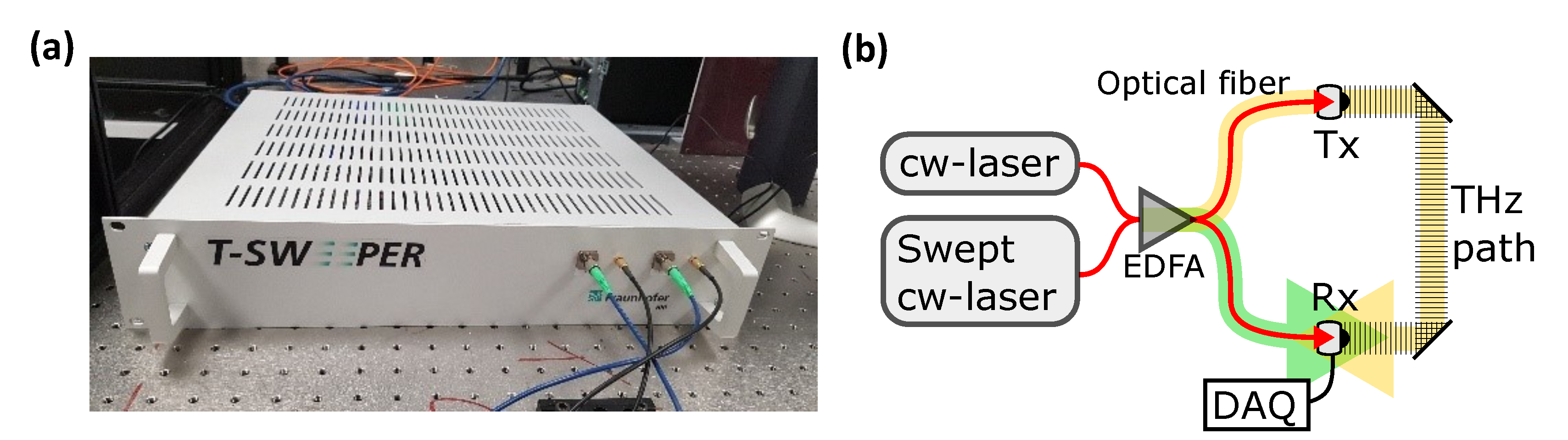
2.1. Operation

The design and operation of the optoelectronic FDS system have been previously reported by Liebermeister et al. [21,22]. As all FDS systems, it uses two fibre-coupled, continuous-wave semiconductor lasers emitting in the c-band (1530–1565 nm) whose frequencies are offset by the desired difference in the THz range. Frequency scanning is achieved by applying a periodic frequency sweep to one of these lasers, while the emission frequency of the second laser stays fixed. The laser outputs are spatially overlapped in a 3 dB coupler, which generates an optical beat note. This beat note is amplified by an erbium-doped fibre amplifier (EDFA) before being converted into THz radiation via photomixing in a waveguide-integrated PIN photodiode emitter. The same beat signal is also used to drive coherent detection in a photoconductive receiver. Both emitter and receiver are based on commercially available, fibre-coupled modules from TOPTICA Photonics AG.

The innovative advance of this system (Figure 1a, which enables it to achieve fast sweep rates and yields unambiguous phase data, is the method employed to obtain the phase. It utilises an optoelectronic adaptation of the FMCW (frequency-modulated continuous-wave) technique [21], which results in passive phase modulation. The tunable cw-laser is frequency swept at more than 500 $\mathrm{T}$$\mathrm{Hz}$/${\mathrm{s}}^{-1}$. In combination with a path length imbalance of 20 cm between the emitter and the receiver arm (indicated by shaded arrows in Figure 1b, an intermediate frequency of 500 $\mathrm{k}$$\mathrm{Hz}$ is generated in the photomixing receiver, which can be directly used for coherent detection with a software-based lock-in amplifier. This quadrature lock-in detection allows one to detect amplitude and phase as a function of frequency. As a consequence, the optoelectronic FMCW systems require neither optomechanical nor electro-optic phase modulation. The frequency resolution of it is 1 $\mathrm{G}$$\mathrm{Hz}$, determined by the cycle time of the sweep laser, which in this case is equal to 2 $\mathsf{\mu }\mathrm{s}$ [21].

As shown in Figure 1b, the THz beam path was a standard configuration of two F/2 parabolic mirrors.

2.2. Other THZ Spectrometers for Comparison Measurements

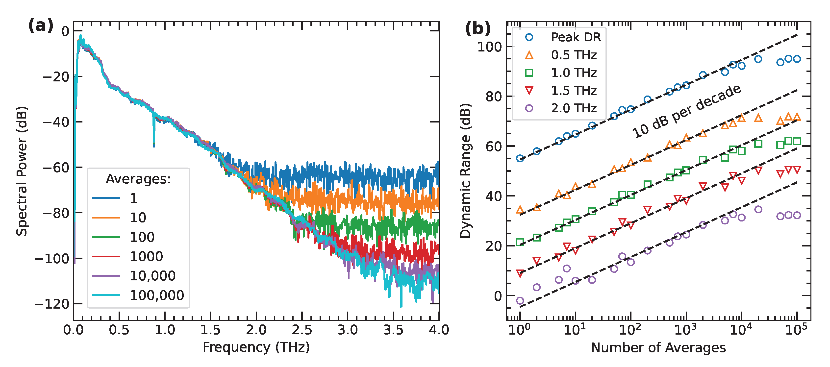
The performance of the T-Sweeper was tested by comparing it with two commercially available THz spectrometer instruments: a TDS and FDS, which had been previously calibrated and validated.

The TDS was a TeraFlash pro from TOPTICA Photonics, employing 1550 $\mathrm{n}$$\mathrm{m}$ fibre laser technology and InGaAs photoconductive switches as the emitter and receiver. The THz beam path was the standard configuration of four F/2 parabolic mirrors; an example of this system’s performance can be observed in [23]. The THz beam path was contained in an enclosure purged with dry air to eliminate absorption by the atmospheric water vapour. The frequency resolution was set to 5 $\mathrm{G}$$\mathrm{Hz}$; and 1000 time-domain averages were used for all measurements. With these settings, the maximum dynamic range was 93 dB, and the cut-off frequency was $5.6$ $\mathrm{T}$$\mathrm{Hz}$.

The FDS was TeraScan from TOPTICA Photonics similarly employing 1550 $\mathrm{n}$$\mathrm{m}$ fibre laser technology and InGaAs photoconductive emitter and receiver. The performance comparison with the optoelectronic FMCW system was further aided by using the same emitter and receiver devices and the same THz beam path in both instruments. The frequency range of the TeraScan is comprised of two bands: 0.1–$1.33$ $\mathrm{T}$$\mathrm{Hz}$ and 1.33–$2.18$ $\mathrm{T}$$\mathrm{Hz}$. The frequency step size was set to 50 $\mathrm{M}$$\mathrm{Hz}$, and the integration time was 3 $\mathrm{m}$$\mathrm{s}$. For the measurements with the FDS systems, the terahertz beam path was contained in an enclosure purged with dry air to eliminate absorption by atmospheric water vapour.

Both TeraFlash pro and TeraScan have been previously calibrated and tested using the same procedures as described below for the T-Sweeper.

2.3. Specifications

In THz spectroscopy, two of the most important instrument specifications are the operational range of frequencies and the frequency-dependent dynamic range (DR). The two parameters are related, because the operational frequency range is defined as the region where DR > 2.

Dynamic range is defined as the ratio or maximum measurable signal ($S_{max}$) and the noise floor (NF): $\mathrm{DR}=S_{max}/\mathrm{NF}$[24]. Dynamic range is important because it represents the range of signal amplitude values that can be measured by the system. As a consequence, it limits the maximum material loss that can be accurately quantified [25]. For TDS and FDS systems, DR is frequency-dependent, because it is proportional to $S_{max}$. DR can be increased by averaging, since it is inversely proportional to NF. For random (Gaussian) noise, averaging lowers the noise floor by a factor of $N^{1/2}$, where N is the number of traces [26]. Due to the spectral profile of the instrument, reducing the noise floor extends the frequency range.

Figure 2 presents the DR of the optoelectronic FMCW system using from 1 to 100,000 averages in steps of a factor of 10. The spectral profile is roughly exponential, as expected in this type of system, falling by 27 dB per terahertz. However, there are some deviations from pure exponential behaviour, which are attributed to emitter and/or receiver geometry. In particular, the sharp dip at $0.88$ $\mathrm{T}$$\mathrm{Hz}$ is a system artifact whose origin is being investigated. Notably, the DR saturates above 20,000 averages due to slow variations and drifts in the environment. In the configuration used in this work, the spectral range is 0.1– 2 $\mathrm{T}$$\mathrm{Hz}$ for a single shot and 0.1–3 $\mathrm{T}$$\mathrm{Hz}$ for 10,000 averages, requiring 24 $\mathrm{m}$$\mathrm{s}$ and 235 $\mathrm{s}$ (around 4 $\min$) scanning time, respectively.

Table 1. Summary of the parameters for the three used devices with the respective settings.

Parameters	T-Sweeper (FDS)	TeraFlash pro (TDS)	TeraScan (FDS)
Measuring Time (min)	≈4	≈2.5	≈80
Frequency Range (THz)	0.1–3	0.1–5.6	0.1–2.18
Frequency Resolution (GHz)	1	5	0.05
${\mathrm{DR}}_{\max }$ (dB)	91	93	83

summarises the essential measurement parameters of the individual devices. These are the results of the selected settings used for the following measurements in Section 3 and Section 4.

3. Calibration of the Optoelectronic FDS-System

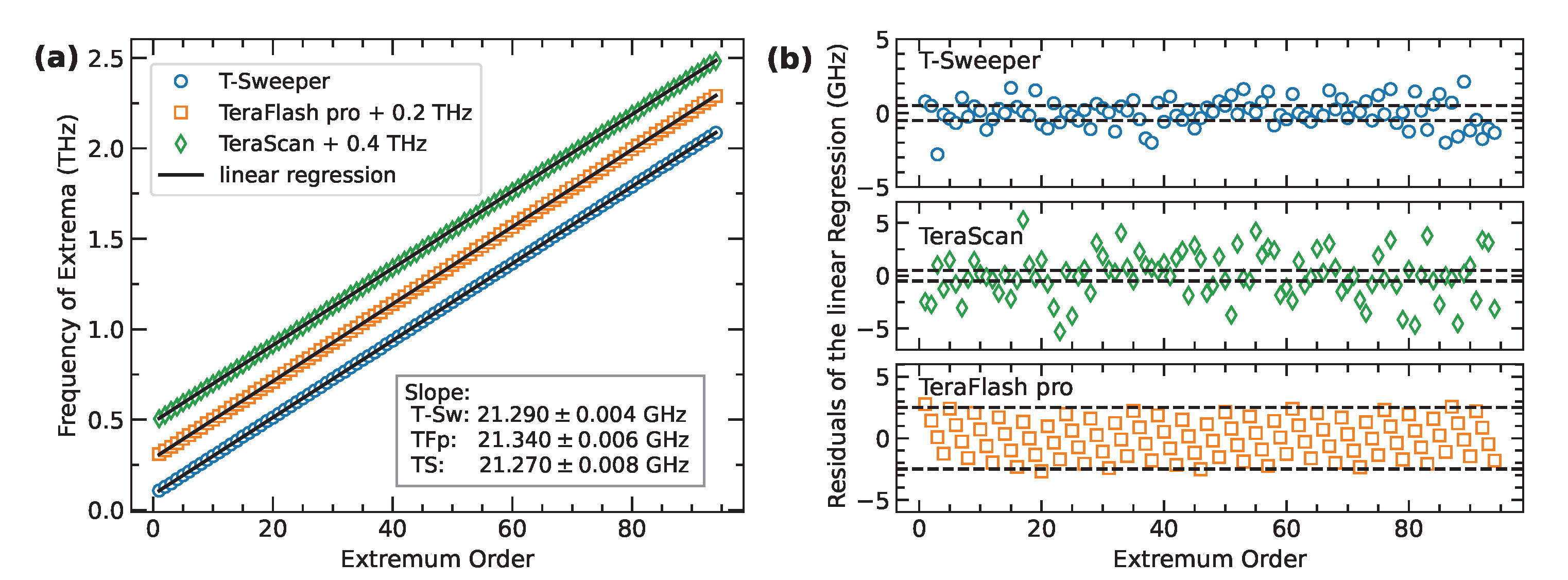
3.1. Frequency Calibration

Frequency is one of the highest-precision quantities measurable by human endeavour. Frequency standards are ultimately traceable to the International Atomic Time Standard based on atomic clocks, providing precision down to ${10}^{-16}$ [27,28]. Accurate frequency determination is obviously important for spectroscopic measurements.

Due to the broadband frequency range of the optoelectronic FDS-System, a frequency calibration standard must have multiple narrow spectral features. A common approach is to employ gas absorption lines, whose frequencies are known with high precision [29]. Atmospheric water vapour provides a convenient set of absorption lines in the 0.5–4 $\mathrm{T}$$\mathrm{Hz}$ range that is widely used for frequency calibration of THz spectrometers. Figure 3a depicts the transmission spectrum through the ambient atmosphere showing water vapour absorption lines, measured by the three devices. Figure 3b plots the deviations of the measured lines from the frequencies listed by HITRAN [29], with results obtained by TeraFlash and TeraScan for comparison. For all three instruments, the deviations are randomly distributed and lie within the uncertainty of their frequency resolution, confirming the accuracy of their frequency scales. It is observed that T-Sweeper demonstrates the smallest deviations from the HITRAN data, due to its high frequency resolution ( 1 $\mathrm{G}$$\mathrm{Hz}$) and low noise. TeraFlash has the largest deviations due to its lowest frequency resolution ( 5 $\mathrm{G}$$\mathrm{Hz}$).

Water vapour lines have the drawback of being unevenly distributed with varying line strengths, sparse below 1 $\mathrm{T}$$\mathrm{Hz}$, and with no suitable lines below $0.5$ $\mathrm{T}$$\mathrm{Hz}$. An alternative approach to frequency calibration is to employ a Fabry-Perot etalon [30,31]. An etalon has the advantage of an evenly spaced comb of equal-amplitude peaks across the whole spectral range of etalon transparency window, allowing systematic errors or drifts in frequency to be easily detected. However, the frequency resolution of an etalon is limited by its finesse, and commonly available etalons are low finesse, providing peaks that are 10–20 $\mathrm{G}$$\mathrm{Hz}$ FWHM (full width at half-maximum). Moreover, an etalon must be calibrated with a frequency standard, for example by using gas absorption lines.

A high-resistivity silicon wafer can serve as a low-finesse etalon [30]. High-resistivity Si has negligible THz absorption and a near-constant refractive index of 3.42 in the range of measurement, and is compact and convenient to use. The free spectral range (FSR) of an etalon is the frequency spacing between successive etalon maxima (or minima). FSR is given by $\mathrm{FSR}=c/nd$, where n is the refractive index of the etalon material and d is its thickness. A Si wafer can thus be chosen to provide the desired FSR.

The transmission spectrum of a Si wafer has been measured and the maxima identified. These occur at frequencies of $f_p=2p·\mathrm{FSR}$, where p is the peak order. The FSR of the etalon can therefore be determined by plotting $f_p$ versus p and applying a linear fit, as shown in Figure 4a. The FSR values obtained were $42.580\pm 0.008$ $\mathrm{G}$$\mathrm{Hz}$ for T-Sweeper, $42.780\pm 0.022$ $\mathrm{G}$$\mathrm{Hz}$ for TeraFlash, and $42.540\pm 0.016$ $\mathrm{G}$$\mathrm{Hz}$ for TeraScan. The values are in agreement within the measurement uncertainty. In order to reveal systematic errors or drifts in the frequency scale, Figure 4b plots the frequency residuals for each instrument, calculated as $0.5f_p-$$p·\mathrm{FSR}$. In the case of T-Sweeper and TeraScan, the residuals are randomly distributed around zero, confirming the absence of systematic frequency errors. The standard deviation of the residuals of the T-Sweeper is smaller than those of TeraScan by a factor of 2.3. In the case of TeraFlash, the residuals follow a saw-tooth pattern arising from coarser frequency resolution; however, they are also evenly distributed around zero.

3.2. Linearity Calibration

Amplitude linearity calibration refers to testing that the measured signal amplitude is linear with the incident signal. This is necessary because many types of instrumental effects can result in non-linear amplitude measurements. Two types of amplitude non-linearity are most frequently observed: (i) amplitude saturation at high signal levels; and (ii) amplitude tail at low signal levels when approaching the noise floor. Amplitude linearity can be tested by employing a series of attenuators of known power, or combinations of attenuators [32,33]. In order to test broadband systems, such as TDS and FDS, attenuators must have frequency-independent attenuation that is accurately known.

Amplitude calibration was performed using a set of high-resistivity Si plates [32]. The normal-incidence amplitude transmission through a Si plate is 0.7; and a stack of N plates will have multiplicative transmission of $0.7^N$ . Thus, a stack of Si plates can provide a variable, controlled, and known attenuation, such as that required for linearity testing. However, it should be noted that Si plates must be tested to verify their refractive index and transparency.

The T-Sweeper had its linearity tested using this method. Figure 5a plots the transmitted amplitude as a function of the number of Si plates placed in the beam path, on a semi-log scale. If the amplitude response is linear, the amplitude would be expected to decrease linearly; the black dashed lines demonstrate the expected slope of 0.7. Figure 5b shows the fitted slopes over the entire spectrum.

It is observed that at all frequencies between 0.1–$2.2$ $\mathrm{T}$$\mathrm{Hz}$ the slopes are close to the expected value of 0.7, with variations within the measurement uncertainty, and the mean value of 0.695 ± 0.021. This linearity calibration method therefore reveals the operational frequency range of the instrument (using the present settings). At higher frequencies, the slopes deviate from linearity when the number of plates exceeds 7, revealing the operational dynamic range limits at these frequencies. Above $2.2$ $\mathrm{T}$$\mathrm{Hz}$ the signal is dominated by noise, especially for a high number of silicon plates.

4. Material Measurement Comparison

4.1. Parameter Extraction

For all three instruments—T-Sweeper, TDS and FDS—the frequency-dependent (f) refractive index ($n\left(f\right)$) and absorption coefficient ($\alpha \left(f\right)$) of material under test can be calculated from the frequency-dependent field amplitude ($E\left(f\right)$) and phase ($\mathsf{\Phi }\left(f\right)$) by using the equations [16,17,18]:

$$n\left(f\right)=\frac{\left({\mathsf{\Phi }}_s\left(f\right)-{\mathsf{\Phi }}_{ref}\left(f\right)\right)c}{2\pi fd}$$

(1)

$$\alpha \left(f\right)=-\frac{2}{d}·ln\left[\frac{{(n+1)}^2}{4n}\frac{E_s\left(f\right)}{E_{ref}\left(f\right)}\right]$$

(2)

where c is the speed of light, d is the sample thickness, and the subscripts s and ref refer to the sample and reference data, respectively. In addition, the maximum measurable absorption is an important parameter in the interpretation for certain samples. The parameter is determined by the dynamic range of the device and represents absorption such that the transmitted amplitude is reduced to the level of the noise floor [23].

$${\alpha }_{max}=\frac{2}{d}·ln\left[DR·\frac{4n}{{(n+1)}^2}\right]$$

(3)

In the case of TDS, the field amplitude ($E\left(f\right)$) and phase ($\mathsf{\Phi }\left(f\right)$) are obtained from the time-domain data by applying Fourier transform. The frequency resolution corresponds to the length of the time-domain scan length.

In the case of the T-Sweeper, the manufacturer’s software (Fraunhofer Heinrich Hertz Institute, Berlin, Germany) outputs the amplitude and phase spectrum. The phase spectrum is wrapped by $-\pi$ to $+\pi$; it is unwrapped using the function of the NumPy library for the python programming language. When interpreting the results of the unwrapping, it should be noted that phase unwrapping can produce errors, especially in combination with noise [18], which must be corrected. The signal data obtained from T-Sweeper is used to calculate the complex transmission function. The magnitude of this corresponds to the transmission in Equation (2) and the argument to the phase difference in Equation (1) [34]. Complex values are used because experience shows that the calculated values, especially the phase, are more accurate using this approach. The measured data of the T-Sweeper and the TeraScan were filtered with a forward and backward digital filter of the Butterworth type. The lowpass Butterworth filter had an order of 5 and a cut-off of 0.1 times the Nyquist frequency.

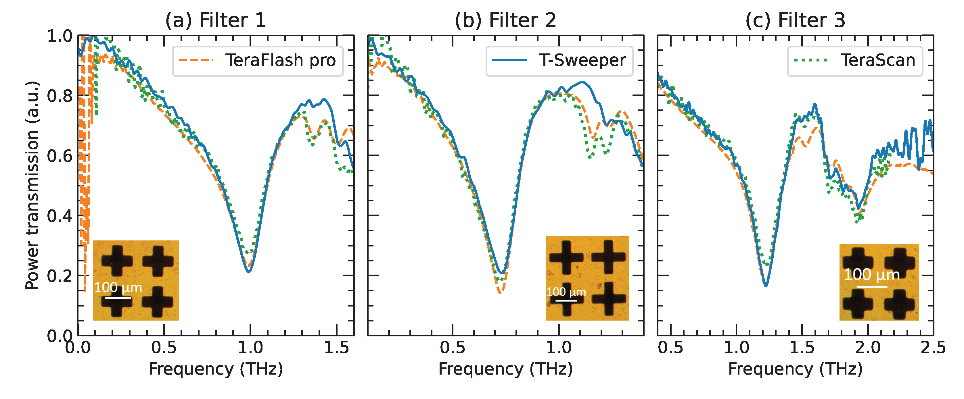
4.2. Resonant Mesh Filters

Resonant mesh filters offer good test materials because they have well-defined spectral features. Such filters typically consist of a thin wafer or film of THz-transparent polymer with deposited or embedded metal pattern of crosses on a square grid. The grid size (g), the size of the crosses (a), and widths of the lines (b) determine the central frequency of the filter and its bandwidth [35]. The filters used in this work were manufactured by Novalia Ltd by printing a 40 $\mathrm{n}$$\mathrm{m}$ thick aluminium structure on a 23 $\mathsf{\mu }$$\mathrm{m}$ thick polyester (PET) substrate. Figure 6 shows the transmission of three of these filters, which were measured with all three instruments.

Overall, the measured transmission spectra for each filter agree well among the devices. There is close agreement in the profile of the loss notch. The slight variations in the notch minima are due to the sensitivity of the filter transmission to their position in the THz beam. For example, a minimum of 0.2359 ± 0.0031 was measured in Filter 3 with TeraScan, compared to a 0.1668 ± 0.0045 with the T-Sweeper. This may be attributed to the fact that the dimensions of the mesh are similar to the wavelength. At higher frequencies, transmission measured by T-Sweeper is slightly above those measured by TeraFlash pro and TeraScan, which may be due to higher noise.

4.3. Lactose Monohydrate

Lactose monohydrate is frequently used in tests of THz spectroscopy due to its characteristic absorption spectrum containing several strong features [36]. The measured sample was a $1.09$ $\mathrm{m}$$\mathrm{m}$ thick pellet. Figure 7 shows the absorption coefficient and refractive index of lactose in the frequency range 0.1–$2.5$ $\mathrm{T}$$\mathrm{Hz}$ for all three devices.

Also plotted (dashed lines) in Figure 7a are the values of maximum measurable absorption for the DR of each instrument [25], showing the limits of measurement. The strong resonance at $1.36$ $\mathrm{T}$$\mathrm{Hz}$ can only be fully captured by TeraFlash, as the other two devices have insufficient dynamic range. Figure 7b shows good agreement in the measured refractive index, except around $0.6$ $\mathrm{T}$$\mathrm{Hz}$ where TeraScan data deviated significantly. The peak in Figure 7c has been examined more closely with the T-Sweeper $0.533$ $\mathrm{T}$$\mathrm{Hz}$, TeraFlash $0.53$ $\mathrm{T}$$\mathrm{Hz}$ and TeraScan $0.534$ $\mathrm{T}$$\mathrm{Hz}$. Figure 7c shows that the spectrum measured by TeraFlash is very similar to that of the T-Sweeper. In contrast to the other two devices, slightly lower absorption is measured by TeraScan, but overall, good agreement is observed among three instruments, in particular between T-Sweeper and TeraFlash.

4.4. Ultra-High Molecular Weight Polyethylene (UHMWPE)

Polyethylene has low THz absorption and is widely used in THz applications. All grades of polyethylene have a prominent absorption peak at around $2.2$ $\mathrm{T}$$\mathrm{Hz}$ that is due to a lattice vibration of the PE molecule [37]. Figure 8 shows the absorption coefficient and refractive index of UHMWPE (d = $10.1$ $\mathrm{m}$$\mathrm{m}$) obtained with the three devices.

Figure 8a shows that the frequency range of TeraScan is insufficient to record the entire absorption peak, with only the low-frequency part being detected. The peak maximum was measured at $2.185$$\mathrm{T}$$\mathrm{Hz}$ by TeraFlash and $2.198$ $\mathrm{T}$$\mathrm{Hz}$ by T-Sweeper. The peak profile measured by the T-Sweeper is skewed at the peak maximum, explaining the difference in the measured peak frequencies. The skewed profile is caused by the noise and the filtering of the signal. Considering the FWHM of the peak, as determined using the Python library SciPy, these are $0.134$ $\mathrm{T}$$\mathrm{Hz}$ for the TeraFlash pro and $0.139$ $\mathrm{T}$$\mathrm{Hz}$ for the T-Sweeper. Figure 8b shows good agreement in the measurements of the refractive index, except at frequencies below $0.5$ $\mathrm{T}$$\mathrm{Hz}$ where the TeraScan deviates significantly. Overall, the measured values of UHMWPE are in good agreement for all three instruments.

5. Conclusions

In this paper, a novel pre-production THz spectrometer was tested and calibrated. The T-Sweeper is a fast-scanning frequency-domain spectrometer designed for industrial applications. It was calibrated, tested and compared with commercially available TDS and FDS instruments, a TeraFlash pro (TDS) and a TeraScan (FDS).

To specify the operation of the T-Sweeper, its operational range of frequencies and the frequency dependent dynamic range have been measured and shown to be 0.1–3 $\mathrm{T}$$\mathrm{Hz}$ and 94 dB, respectively, when using 10,000 measurement averages. Frequency calibration was performed using atmospheric water vapour and a silicon wafer etalon, confirming that the T-Sweeper has a linear frequency axis with no offsets or drift. Amplitude linearity was tested using a set of silicon plates, confirming that the amplitude axis of the T-Sweeper is linear up to the limits of its dynamic range.

In addition, spectroscopy measurements were carried out comparing the performance of the T-Sweeper with TeraFlash and TeraScan, using several types of material samples (resonant mesh filters, lactose monohydrate and UHMWPE). The T-Sweeper performance was observed to be repeatable and in good agreement with other devices, within its range of operation and within measurement uncertainty.

T-Sweeper was confirmed as an accurate, reliable instrument, with good repeatability, suitable for industrial use case scenarios.

References

1. Fuse, N.; Takahashi, T.; Ohki, Y.; Sato, R.; Mizuno, M.; Fukunaga, K. Terahertz spectroscopy as a new tool for insulating material analysis and condition monitoring. IEEE Electr. Insul. Mag. 2011, 27, 26–35. [Google Scholar] [CrossRef]
2. Puc, U.; Abina, A.; Rutar, M.; Zidanšek, A.; Jeglič, A.; Valušis, G. Terahertz spectroscopic identification of explosive and drug simulants concealed by various hiding techniques. Appl. Opt. 2015, 54, 4495–4502. [Google Scholar] [CrossRef] [PubMed]
3. Wietzke, S.; Jansen, C.; Reuter, M.; Jung, T.; Kraft, D.; Chatterjee, S.; Fischer, B.; Koch, M. Terahertz spectroscopy on polymers: A review of morphological studies. J. Mol. Struct. 2011, 1006, 41–51. [Google Scholar] [CrossRef]
4. Komandin, G.; Zaytsev, K.; Dolganova, I.; Nozdrin, V.; Chuchupal, S.; Anzin, V.; Spektor, I. Quantification of solid-phase chemical reactions using the temperature-dependent terahertz pulsed spectroscopy, sum rule, and Arrhenius theory: Thermal decomposition of α-lactose monohydrate. Opt. Express 2022, 30, 9208–9221. [Google Scholar] [CrossRef]
5. Abdul-Munaim, A.M.; Aller, M.M.; Preu, S.; Watson, D.G. Discriminating gasoline fuel contamination in engine oil by terahertz time-domain spectroscopy. Tribol. Int. 2018, 119, 123–130. [Google Scholar] [CrossRef]
6. Lin, H.; Russell, B.P.; Bawuah, P.; Zeitler, J.A. Sensing water absorption in hygrothermally aged epoxies with terahertz time-domain spectroscopy. Anal. Chem. 2021, 93, 2449–2455. [Google Scholar] [CrossRef]
7. Neu, J.; Rahm, M. Terahertz time domain spectroscopy for carrier lifetime mapping in the picosecond to microsecond regime. Opt. Express 2015, 23, 12900–12909. [Google Scholar] [CrossRef]
8. Alberding, B.G.; Thurber, W.R.; Heilweil, E.J. Direct comparison of time-resolved terahertz spectroscopy and Hall Van der Pauw methods for measurement of carrier conductivity and mobility in bulk semiconductors. JOSA B 2017, 34, 1392–1406. [Google Scholar] [CrossRef]
9. Naftaly, M.; Vieweg, N.; Deninger, A. Industrial applications of terahertz sensing: State of play. Sensors 2019, 19, 4203. [Google Scholar] [CrossRef]
10. Ellrich, F.; Bauer, M.; Schreiner, N.; Keil, A.; Pfeiffer, T.; Klier, J.; Weber, S.; Jonuscheit, J.; Friederich, F.; Molter, D. Terahertz quality inspection for automotive and aviation industries. J. Infrared Millim. Terahertz Waves 2020, 41, 470–489. [Google Scholar] [CrossRef]
11. True, J.; Xi, C.; Jessurun, N.; Ahi, K.; Asadizanjani, N. Review of THz-based semiconductor assurance. Opt. Eng. 2021, 60, 060901. [Google Scholar] [CrossRef]
12. Tao, Y.H.; Fitzgerald, A.J.; Wallace, V.P. Non-contact, non-destructive testing in various industrial sectors with terahertz technology. Sensors 2020, 20, 712. [Google Scholar] [CrossRef]
13. Ye, D.; Wang, W.; Zhou, H.; Huang, J.; Wu, W.; Gong, H.; Li, Z. In-situ evaluation of porosity in thermal barrier coatings based on the broadening of terahertz time-domain pulses: Simulation and experimental investigations. Opt. Express 2019, 27, 28150–28165. [Google Scholar] [CrossRef]
14. Krimi, S.; Klier, J.; Jonuscheit, J.; von Freymann, G.; Urbansky, R.; Beigang, R. Highly accurate thickness measurement of multi-layered automotive paints using terahertz technology. Appl. Phys. Lett. 2016, 109, 021105. [Google Scholar] [CrossRef]
15. Sun, J.; Hu, F. Three-dimensional printing technologies for terahertz applications: A review. Int. J. Microw.-Comput.-Aided Eng. 2020, 30, e21983. [Google Scholar] [CrossRef]
16. Coutaz, J.L.; Garet, F.; Wallace, V.P. Principles of Terahertz Time-Domain Spectroscopy; CRC Press: Boca Raton, FL, USA, 2018. [Google Scholar]
17. Neu, J.; Schmuttenmaer, C.A. Tutorial: An introduction to terahertz time domain spectroscopy (THz-TDS). J. Appl. Phys. 2018, 124, 231101. [Google Scholar] [CrossRef]
18. Withayachumnankul, W.; Naftaly, M. Fundamentals of measurement in terahertz time-domain spectroscopy. J. Infrared Millim. Terahertz Waves 2014, 35, 610–637. [Google Scholar] [CrossRef]
19. Safian, R.; Ghazi, G.; Mohammadian, N. Review of photomixing continuous-wave terahertz systems and current application trends in terahertz domain. Opt. Eng. 2019, 58, 110901. [Google Scholar] [CrossRef]
20. TeraScan 780/1550 Topsellers for Frequency—Domain SpectroscopyBrochures; TOPTICA Photonics AG: Gräfelfing, Munich, Germany, 2022.
21. Liebermeister, L.; Nellen, S.; Kohlhaas, R.B.; Lauck, S.; Deumer, M.; Breuer, S.; Schell, M.; Globisch, B. Optoelectronic frequency-modulated continuous-wave terahertz spectroscopy with 4 THz bandwidth. Nat. Commun. 2021, 12, 1071. [Google Scholar] [CrossRef]
22. Liebermeister, L.; Nellen, S.; Kohlhaas, R.B.; Lauck, S.; Deumer, M.; Breuer, S.; Schell, M.; Globisch, B. Terahertz Multilayer Thickness Measurements: Comparison of Optoelectronic Time and Frequency Domain Systems. J. Infrared Millim. Terahertz Waves 2021, 42, 1153–1167. [Google Scholar] [CrossRef]
23. Naftaly, M.; Gregory, A. Terahertz and Microwave Optical Properties of Single-Crystal Quartz and Vitreous Silica and the Behavior of the Boson Peak. Appl. Sci. 2021, 11, 6733. [Google Scholar] [CrossRef]
24. Naftaly, M.; Dudley, R. Methodologies for determining the dynamic ranges and signal-to-noise ratios of terahertz time-domain spectrometers. Opt. Lett. 2009, 34, 1213–1215. [Google Scholar] [CrossRef]
25. Jepsen, P.U.; Fischer, B.M. Dynamic range in terahertz time-domain transmission and reflection spectroscopy. Opt. Lett. 2005, 30, 29–31. [Google Scholar] [CrossRef]
26. Taylor, J. Introduction to Error Analysis, the Study of Uncertainties in Physical Measurements; Univerity Science Books: Sausalito, CA, USA, 1997. [Google Scholar]
27. Katori, H. Tricks for ticks. Nat. Phys. 2017, 13, 414. [Google Scholar] [CrossRef]
28. Baynham, C.F.; Godun, R.M.; Jones, J.M.; King, S.A.; Nisbet-Jones, P.B.; Baynes, F.; Rolland, A.; Baird, P.E.; Bongs, K.; Gill, P.; et al. Absolute frequency measurement of the optical clock transition in with an uncertainty of using a frequency link to international atomic time. J. Mod. Opt. 2018, 65, 585–591. [Google Scholar] [CrossRef]
29. Gordon, I.; Rothman, L.; Hargreaves, R.; Hashemi, R.; Karlovets, E.; Skinner, F.; Conway, E.; Hill, C.; Kochanov, R.; Tan, Y.; et al. The HITRAN2020 molecular spectroscopic database. J. Quant. Spectrosc. Radiat. Transf. 2022, 277, 107949. [Google Scholar] [CrossRef]
30. Naftaly, M.; Dudley, R.; Fletcher, J. An etalon-based method for frequency calibration of terahertz time-domain spectrometers (THz TDS). Opt. Commun. 2010, 283, 1849–1853. [Google Scholar] [CrossRef]
31. Kinoshita, M.; Iida, H.; Shimada, Y. Frequency calibration of terahertz time-domain spectrometer using air-gap etalon. IEEE Trans. Terahertz Sci. Technol. 2014, 4, 756–759. [Google Scholar] [CrossRef]
32. Naftaly, M.; Dudley, R. Linearity calibration of amplitude and power measurements in terahertz systems and detectors. Opt. Lett. 2009, 34, 674–676. [Google Scholar] [CrossRef]
33. Iida, H.; Kinoshita, M. Amplitude Calibration in Terahertz Time-Domain Spectroscopy Using Attenuation Standards. J. Infrared, Millimeter, Terahertz Waves 2018, 39, 120–129. [Google Scholar] [CrossRef]
34. Duvillaret, L.; Garet, F.; Coutaz, J.L. A reliable method for extraction of material parameters in terahertz time-domain spectroscopy. IEEE J. Sel. Top. Quantum Electron. 1996, 2, 739–746. [Google Scholar] [CrossRef]
35. Melo, A.M.; Gobbi, A.L.; Piazzetta, M.H.; Da Silva, A.M. Cross-shaped terahertz metal mesh filters: Historical review and results. Adv. Opt. Technol. 2012, 2012, 530512. [Google Scholar] [CrossRef]
36. Roggenbuck, A.; Schmitz, H.; Deninger, A.; Mayorga, I.C.; Hemberger, J.; Güsten, R.; Grüninger, M. Coherent broadband continuous-wave terahertz spectroscopy on solid-state samples. New J. Phys. 2010, 12, 043017. [Google Scholar] [CrossRef]
37. Sommer, S.; Raidt, T.; Fischer, B.M.; Katzenberg, F.; Tiller, J.C.; Koch, M. THz-spectroscopy on high density polyethylene with different crystallinity. J. Infrared Millim. Terahertz Waves 2016, 37, 189–197. [Google Scholar] [CrossRef]
Figure 1. T-Sweeper. (a) Photograph of the instrument. (b) Schematic drawing of instrument operation, components, and the optical and THz beam paths. Extracted from [22]. Tx—transmitter; Rx—receiver; DAQ—data acquisition.
Applsci 12 08257 g001
Figure 2. (a) Spectral power and dynamic range using 1 to 100,000 averages. (b) The dynamic range at the peak and at four selected frequencies as a function of number of averages, showing the 10 per decade slope (dashed lines) and saturation above 20,000 averages.
Applsci 12 08257 g002
Figure 3. (a) Absorption spectrum of atmospheric water vapour measured by T-Sweeper, TDS and FDS. The grey vertical lines correspond to the values from HITRAN. (b) Deviations of the measured lines from the line data listed by HITRAN [29].
Applsci 12 08257 g003
Figure 4. (a) Frequency of the peak maxima plotted versus peak order, with the linear fit for all three devices. For clarity, values of the TeraScan and TeraFlash pro have been offset. The slopes of linear regression are shown in the bottom right inset. Since this is the distance between the successive minima and maxima, this must be doubled for the calculation of FSR (cf. above). (b) Frequency residuals of extreme values, measured with T-Sweeper, TeraFlash and TeraScan. The dashed lines represent half the frequency resolution.
Applsci 12 08257 g004
Figure 5. (a) Measured transmitted amplitude as a function of the number of Si plates, for different frequencies. Dashed lines show the expected slope. (b) The fitted slopes for all frequencies up to 2.7 T Hz . For clarity, only every 20th datapoint is shown.
Applsci 12 08257 g005
Figure 6. Measured transmission spectra of three resonant mesh filters, using all three instruments. The filter notch frequency is around 0.99 T Hz for Filter 1, 0.73 T Hz for Filter 2, and 1.22 T Hz for Filter 3. Insets show microscope images of each filter, showing the differences in mesh dimensions.
Applsci 12 08257 g006
Figure 7. Absorption coefficient (a) and refractive index (b) of a lactose pellet measured with all three devices. The absorption graph also includes the maximum measurable absorption (cf. Equation (3)); the intersection of α m a x with the measured absorption curve shows the limits of measurement for each instrument. (c) Expanded absorption feature at 0.53 T Hz .
Applsci 12 08257 g007
Figure 8. Absorption coefficient (a) and refractive index (b) of UHMWPE measured by TeraFlash, T-Sweeper, and the TeraScan. The narrow range of values measured reveals the noise in the extracted parameters.
Applsci 12 08257 g008