Research on Image Matching of Improved SIFT Algorithm Based on Stability Factor and Feature Descriptor Simplification

Abstract

In view of the problems of long matching time and the high-dimension and high-matching rate errors of traditional scale-invariant feature transformation (SIFT) feature descriptors, this paper proposes an improved SIFT algorithm with an added stability factor for image feature matching. First of all, the stability factor was increased during construction of the scale space to eliminate matching points of unstable points, speed up image processing and reduce the dimension and the amount of calculation. Finally, the algorithm was experimentally verified and showed excellent results in experiments on two data sets. Compared to other algorithms, the results showed that the algorithm proposed in this paper improved SIFT algorithm efficiency, shortened image-processing time, and reduced algorithm error.

1. Introduction

Image matching [1,2] is one of the important research contents in computer vision and image processing, and is widely used in visual 3D reconstruction [3], tracking [4], object recognition [5] and content-based image retrieval [6]. Its purpose is to find one or more transformations in the transformation space so that two or more images of the same scene from different times, different sensors or different perspectives are spatially consistent. There are many types of image matching methods, among which feature-based matching has better robustness to image distortion, noise and occlusion. However, this matching depends to a large extent on the quality of feature extraction. One of the research hotspots is pattern recognition [7,8,9,10]. The most basic one is the scale-invariant feature transform (SIFT) algorithm proposed by Lowe in 2004 [11,12]. However, it only considers the Euclidean distance between the feature vectors when matching, and does not use any structural information contained in the dataset itself; therefore, the search efficiency is relatively low. When the image noise or the difference between matching objects is large, the mismatching situation is obvious. To solve this problem, Ooi and Weinberger proposed using a Kd tree to divide the space and then perform a nearest neighbor query [13,14], but this means of establishing an index structure carries a relatively high cost. Chen and Torr proposed the M estimation method [15] and the maximum likelihood estimation by sample and consensus (MLESAC) [16] algorithm to estimate the matching matrix. The M estimation method relies completely on the linear least squares method, so the initial value of the estimated matrix low accuracy and poor stability; the MLESAC algorithm is incapable of modeling outliers and has low estimation accuracy. In response to these problems, Choi proposed a better performance random sample consensus (RANSAC) algorithm [17] to purify the matching pairs consistently. Since RANSAC depends on the setting of the number of iterations, the results have errors and may not be optimal. At present, researchers have proposed a variety of description methods for local feature regions of images, such as descriptors based on Gaussian differentiation, invariant moments, controllable filters, time-frequency, pixel gray value distribution or pixel gradient value distribution. Of these methods, the most concerned is Lowe’s SIFT descriptor.

The construction of this feature descriptor is achieved by establishing a three-dimensional gradient directional histogram for the neighborhood of feature points. The SIFT feature is not only invariant to the scale change and rotation of the image, but also has strong adaptability to the illumination change and image deformation and has a high discrimination ability. On this basis, researchers have improved and extended SIFT features, such as the PCA-SIFT descriptor proposed by Ke and Sukthankar [18], and the Gradient location-orientation histogram (GLOH) descriptor proposed by Mikolajczyk and Schmid [19], the Rotation-invariant feature transform (RIFT) descriptor proposed by Lazebnik [20] and the Speeded up robust features (SURF) descriptor proposed by Bay [21].

In the literature, [22] the performance of descriptors similar to SIFT was found to be the best after evaluating the performance of many representative descriptors. Local binary pattern (LBP) is one of the more effective texture analysis features for two-dimensional images [23]. It is essentially a texture descriptor based on pixel gray order that uses local patterns as texture primitives for analysis.

It has the characteristics of simple calculation and invariance to linear illumination changes, and has been widely used in face recognition, background extraction and image retrieval [24,25,26,27]. Reference [28] was the first to apply an LBP operator to the construction of local image feature descriptors, and proposed a Centersymmetric local binary pattern (CS-LBP) local image feature area description method. Experimental results showed that the CS-LBP descriptor has better image matching than the SIFT descriptor and has obvious storage advantages since the SIFT has color space requirements and computational overhead.

Tan and Triggs extended the LBP operator to a ternary code and proposed a Local trinary pattern (LTP) operator [29]. The LTP feature has stronger discrimination than the LBP feature, but its histogram dimension is greatly increased, which is not suitable for directly describing the local feature area of the image. Extending the CS-LBP descriptor directly to the Center symmetric local trinary pattern (CS-LTP) descriptor reduces the dimensionality of the descriptor to a certain extent, but it still cannot meet the needs of practical applications.

There are many derivatives algorithms based on the SIFT algorithm: the GLOH, proposed by Mikolajczyk [30]; the CSIFT, proposed by AbdelHakim [31]; the ASIFT, proposed by Morel [32]; the simplified SSIFT proposed by Liu Li [33]; the PSIFT proposed by Cai Guorong [34]; local feature description based on Laplace, proposed by Tang Yonghe [35]; and image matching based on the adaptive redundant keypoint elimination method in the SIFT [36], the efficiency of SIFT still has a lot of room for improvement.

To address the SIFT algorithm’s poor real-time performance, this paper first changed the scale space calculation method and then added a stability factor to reduce the matching error and calculation time; then, by establishing the feature descriptor of the cross-shaped partition, the dimension of the descriptor was reduced from 128 to 96, which reduced the amount of matching calculation and shortened the matching time.

The structure of the rest of the article is arranged as follows: Section 2 presents the original and Section 3 the improved SIFT algorithm. Section 4 analyzes the experimental results, and Section 5 presents the conclusions.

2. Original SIFT Algorithm

The traditional SIFT algorithm is divided into four parts: scale space extreme value detection, key localization, orientation determination, and key point description.

2.1. Scale Space Extreme Value Detection

Potentially sensitive points that are invariant to scale and rotation are identified using differential Gaussian functions. The scale space of the image is mainly obtained by convolving the Gaussian differential function and the original image, as shown in Equations (1) and (2) [12]:

$$G(x,y,z)=\frac{1}{2\pi {\delta }^2}{e}^{\frac{(x-\frac{m}{2}{)}^2+{(y-\frac{n}{2})}^2}{2{\delta }^2}}$$

(1)

$$L(x,y,\delta )=G(x,y,z)\times I(x,y)$$

(2)

where is $L(x,y,\delta )$ is the scale space function, and $G(x,y,z)$ is the Gaussian blur function. $I(x,y)$ is the original image function, where $(x,y)$ are the image pixel coordinates; $\delta$ is the spatial scale; and $(m,n)$ is the image dimension.

The difference of Gaussian (DoG) detection was used to find the space extremum detection, as shown in Equation (3):

$$D(x,y,\delta )=\left(G\right(x,y,k\delta )-G(x,y,\delta \left)\right)\times I(x,y)=L(x,y,k\delta )-L(x,y,\delta )$$

(3)

In the equation, k is the multiplication factor, and S is the integer number [36]. The value of k is shown in Formula (4):

$$k=2^{\frac{1}{s}}$$

(4)

The key points composed of local extreme points in the DoG space are initially detected by comparing the images of two adjacent layers of each DoG space in the same group. In order to find the extreme point in DoG space, each pixel is compared with all its neighbors to see if it is larger or smaller than its neighbors in the image domain and scale domain. As shown in Figure 1, the detection point in the middle (the “X” in the picture) is compared with its 8 adjacent points of the same scale and the 9 × 2 points corresponding to the upper and lower adjacent scales, a total of 26 points, to ensure that extreme points are detected in both scale space and 2D image space.

2.2. Key Point Positioning

The extreme point in the discrete space is not the real extreme point. The method of using known discrete space point interpolation to obtain the continuous space extreme point is called sub-pixel interpolation.

To improve the stability of key points, curve fitting was performed on the scale-space DoG function. Using the Taylor expansion of the function in the scale space:

$$D\left(x\right)=D+\frac{\partial D^T}{\partial X}X+\frac{1}{2}{X}^T\frac{{\partial }^{2}D}{\partial X^2}X$$

(5)

In the formula, the key points obtained by $X={(x,y,\delta )}^T$ generated a strong edge response, so the unstable edge response points needed to be eliminated so that the threshold could be set.

2.3. Direction Determination

After the key points were found, considering that they are in the scale space, it was necessary to use local image features to assign a reference direction to all key points so that the descriptor had rotation invariance. Therefore, the image gradient method was used to obtain the stable direction of the local structure. The magnitude and direction of the gradient are shown in Equations (6) and (7):

$$m(x,y)=\sqrt{{(L(x+1,y)-L(x-1,y))}^2+{(L(x,y+1)-L(x,y-1))}^2}$$

(6)

$$\theta (x,y)=ta{n}^{-1}\left(((L(x,y+1)-L(x,y-1))/(L(x+1,y)-L(x-1,y)))\right)$$

(7)

where $m(x,y)$ is the gradient value; L is the scale space value where the key point is located; and $\theta$ is the gradient direction. The histogram was used to count the gradient directions of the key point in a certain neighborhood, find the direction corresponding to the highest histogram peak and then use it as the main direction of the key point.

2.4. Description of Key Points

Three pieces of information were obtained from the above: position, scale, and orientation. A descriptor was then established for each key point, and a set of vectors was used to describe the key point so that it did not change because of changes in lighting or perspective. This descriptor included not only the key points, but also the pixels around the key points that affected it. At the same time, the descriptor had to have uniqueness to improve the probability of correctly matching of feature points. The generation of keypoint descriptors is shown in Figure 2. The red dots in Figure 2 represent feature points. First, a square pixel area of a 16 × 16 grid was selected around the feature points; second, the 4 × 4 grid was divided; finally, the cumulative gradient values of 8 directions (one direction every 45 degrees) were calculated in each sub-region, and each feature point generated a 4 × 4 × 8 (128) dimensional feature descriptor.

As above, the 4 × 4 × 8 = 128 gradient information was the feature vector of the key point. To remove the influence of illumination changes after the eigenvectors were formed, they had to be normalized. The normalized eigenvectors are shown in Formula (8):

$$w_i=\frac{f_i}{\sqrt{{\displaystyle \sum _{j=1}^{128}}{f}_j}}$$

(8)

where $w_i$ is the normalized vector; $f_i$ is the original feature vector; and $j=1,2,3\cdots$. Larger gradient values were truncated by setting the threshold value. After that, a normalization process was performed to improve the discrimination of the features.

3. Improved SIFT Algorithm

To address the low real-time performance of the SIFT algorithm, two innovations were proposed in this paper: increase the stability factor in the scale space and simplify the feature descriptor. This section describes these improvements.

3.1. Scale Space Increases the Stability Factor

The traditional scale space construction formula is

$$\delta (o,s)={\delta }_0{2}^{o+\frac{s}{S}},oϵ[0,\cdots ,O-1],sϵ[0,\cdots ,S+2]$$

(9)

where $\delta$ is the scale space coordinate; O is the number of octaves; S is the number of layers in the group; ${\delta }_0$ is the scale of the reference layer; o is the index of the octave of the group; and s is the index of the layer in the group.

When building the Gaussian pyramid at the beginning, the input image should be pre-blurred as the image of the 0th layer of the 0th group, which is equivalent to discarding the highest sampling rate of the spatial domain. Therefore, the usual practice is to double the scale of the image to generate the −1 group. Apply a Gaussian blur of ${\delta }_{-1}=0.5$ to it, if the size of the input image is doubled with bilinear interpolation, then it is equivalent ${\delta }_{-1}=1$.

When constructing a Gaussian pyramid, the scale coordinates of each layer in the group are calculated as follows:

$$\delta \left(s\right)=\sqrt{{\left(k^s{\delta }_0\right)}^2-{\left(k^{s-1}{\delta }_0\right)}^2}$$

(10)

The value of k is shown in Formula (4).

To reduce error and matching time, a stabilizer P is added, and then a new Gaussian pyramid is constructed. The scale coordinates of each layer in the group are calculated as follows:

$$\delta \left(s\right)=\sqrt{{\left(w^s{\delta }_0\right)}^2-{\left(w^{s-1}{\delta }_0\right)}^2}$$

(11)

Definition 1.

Stabilizer factor P

To reduce error and matching time, the stabilizer P is added, where $P=\frac{w}{k}$. The stabilizer factor P is shown in Equation (12):

$$P=0.4^S+0.9$$

(12)

Proof. 

Because the number under the square root of formula (11) is greater than or equal to 0:

$${\left(w^s{\delta }_0\right)}^2-{\left(w^{s-1}{\delta }_0\right)}^2\ge 0.$$

(13)

According to [36], ${\delta }_0=1.6$, so

$${\left(w^s\right)}^2-{\left(w^{s-1}\right)}^2\ge 0.$$

(14)

According to $w=pk$, so

$${\left(p^s{k}^s\right)}^2-{\left(p^{s-1}{k}^{s-1}\right)}^2\ge 0.$$

(15)

Since the value of $k>0 and p>0$,

$$\left(p^2{k}^2\right)\ge 1.$$

(16)

According to [36], usually $3\le S\le 5$, so

$$P>\frac{1}{2^{\frac{1}{S}}}\ge 0.87,$$

(17)

and because we want to remove redundant feature points, if $P<1$, then $0.87\le P<1$.

Since k is a decreasing function, so must w be; k is also an exponential function. To facilitate the derivation, P was designed as an exponential function as follows:

$$P=A^S+b$$

(18)

To ensure that P is a decreasing function, let $0<A<1$. When S is infinite, $AS=0 and P=B$. To ensure that the value of P can remove redundant points, let $B=0.9$ because $0.87\le P<1$, $A^S$ needs to meet $0<A^S<1$. Usually $3\le S\le 5$, so

$$0<A^S<0.1^{\frac{1}{3}}<0.47.$$

(19)

Let $A=0.4$ to ensure that the filtering window and feature points are not too small.

Therefore, $P=0.4^S+0.9$. □

3.2. Simplified Feature Descriptor

In the original SIFT algorithm, there were 128 high-dimensional feature descriptors and redundant data. The computational complexity of computing the feature descriptor is

$$O(keypoints.size\times d1\times d2\times (n^2+scal{e}^2))$$

(20)

where $O\left(\right)$ represents the time complexity of the corresponding algorithm; $keypoints.size$ represents the number of feature points; $d_1$ and $d_2$ represent the dimension of the feature descriptor; n represents the number of iterations of the algorithm; and $scale$ represents the Gaussian scale. The time complexity of the 128 dimensions is

$$O(keypoints.size\times 4\times 4\times (n^2+8^2)).$$

(21)

The higher the dimension of the feature descriptor, the higher the time complexity. Therefore, this article simplified the descriptor. The specific division of the simplified descriptor is shown in Figure 3, the red dots in Figure 3 represent feature points. Compared with the square area divided by the SIFT algorithm, the $4\times 4$ grid pixels with 4 corners were discarded. The basis for this was that the smaller the distance between the pixel and the feature point, the smaller the contribution to the matching. The the weight distribution of the descriptor data was in line with the Gaussian kernel, so the pixel information that was far away and had little influence on the matching effect was discarded. Therefore, obtaining a 3 × 4 × 8 (96)-dimensional feature descriptor reduced the descriptor dimension of the original SIFT algorithm by 25%. The time complexity of 96 dimensions is

$$O(keypoints.size\times 3\times 4\times (n^2+8^2)),$$

(22)

so the consumption time was shortened, and the computational complexity and amount of computation of the algorithm was reduced. Although a small amount of feature information in the corners was discarded, the uniqueness of the descriptor improved, and the matching of feature points with the same name was faster and more stable.

If $T=(t_1,t_2,\cdots ,t_{96})$ is a 96-dimensional feature descriptor of a feature point, it needs to be normalized to remove the influence of illumination changes.

Definition 2.

Normalized feature vector According to Formula (8) and the 96-dimensional feature descriptor model, the improved normalized feature vector is shown in Formula (21):

$$\overline{t_i}=\frac{t_i}{\sqrt{{\displaystyle \sum _{j=1}^{96}}{t}_j}}$$

(23)

Therefore, the feature descriptor $\overline{T}=(\overline{t_1},\overline{t_2},\cdots ,\overline{t_{9}6})$ was obtained.

4. Experimental Results and Analysis

4.1. Experimental Environment

To show the adaptability of this algorithm to different types of datasets, two different types were selected: The first was the kitti dataset, which is used in unmanned driving, which is closer to the real perspective of mobile robots and unmanned vehicles, and it is close to life scenes. The second was the Euroc dataset, which is collected in the factory environment, close to the industrial scene. The kitti dataset contained 20 sets of pictures, the pixel size of which was 1242 × 375. The Euroc dataset contained 20 pictures, the pixel size of which were 752 × 480. The purpose of selecting these two datasets was to show the effect of the algorithm in this paper on life and industrial scenes. It had good authenticity.

The experimental equipment in this paper was a Legion Y7000p laptop, equipped with an Inte(R) Core(TM) i7-10750H CPU, a frequency of 2.6 GHz, and 16 G of memory. The programming platform was VS2019; the language was C++; and the operating system was 64-bit Windows 10.

4.2. Comparison of Experimental Results

4.2.1. Comparison of Experimental Results Based on Kitti Dataset

Indicator description: RN represented the number of reference image feature points; WN: the number of image feature points to be matched; MN: the number of matching points; PT: the matching time; and rems represented the rems error.

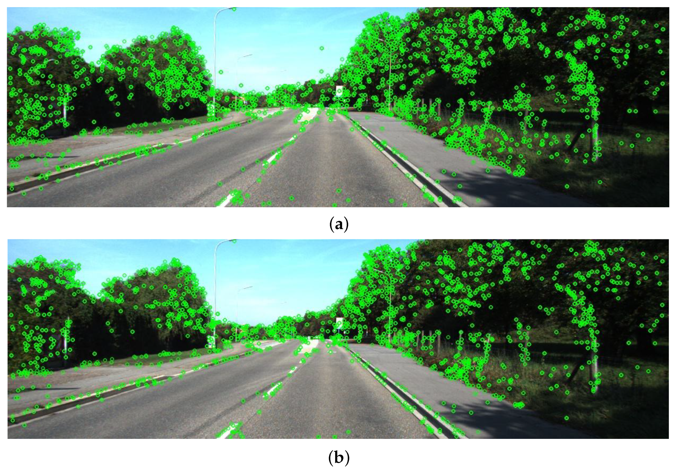
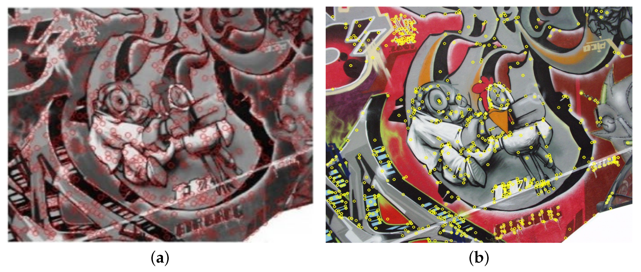
First, the Kitti dataset was used, and the feature point extraction results of a group of pictures were randomly selected for display. These included reference images and images to be registered. The serial number in the dataset was 17). The feature-point extraction results of the SIFT algorithm of the reference image and the algorithm of this paper are shown in Figure 4; the results of the SIFT algorithm of the image to be registered and the algorithm of this paper are shown in Figure 5. Of these, Figure 4a and Figure 5a are the feature points extracted by the SIFT algorithm, and Figure 4b and Figure 5b are those extracted by the algorithm in this paper, which increased the stability factor and simplified the description. The number of feature points obtained by the algorithm was reduced Figure 4a. The number of feature points extracted by the SIFT algorithm was 6203. After optimization by the algorithm in this paper, the number of feature points in Figure 4b was 4725. The number of features extracted by the SIFT algorithm in Figure 5a was 4348, and the number optimized by the algorithm in this paper was 3429. From Figure 4 and Figure 5, the feature points extracted by the algorithm were also sparser than those of the SIFT algorithm, which proved the role of the stability factor.

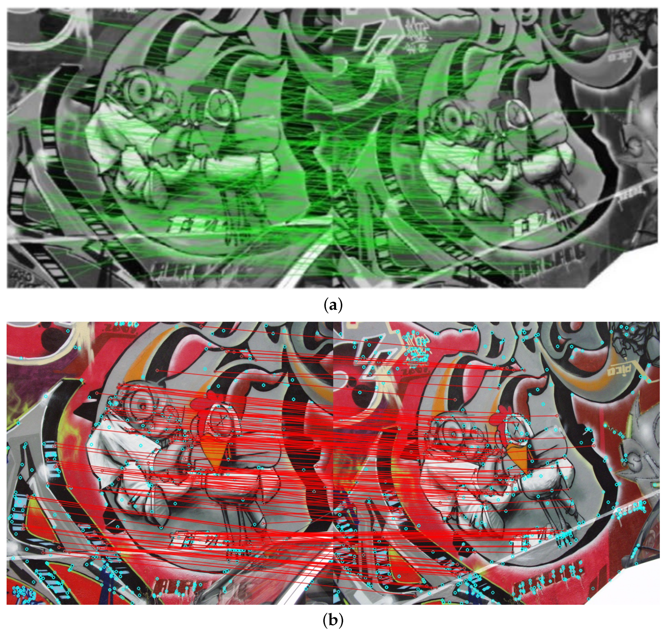
The matching results of the reference image and the image to be registered are shown in Figure 6, and the matching results of the SIFT algorithm are shown in Figure 6a. The matching time of the SIFT algorithm was 3.284 s with a root mean square error of 0.153. Using the feature descriptor to remove the four-corner rectangular area made the feature description ability faster and eliminated some less ideal matching point pairs. The matching results of the optimized algorithm are shown in Figure 6b. The matching time of the algorithm was 2.63 s, with a root mean square error of 0.122, which proved the advantage of this algorithm in this group of pictures.

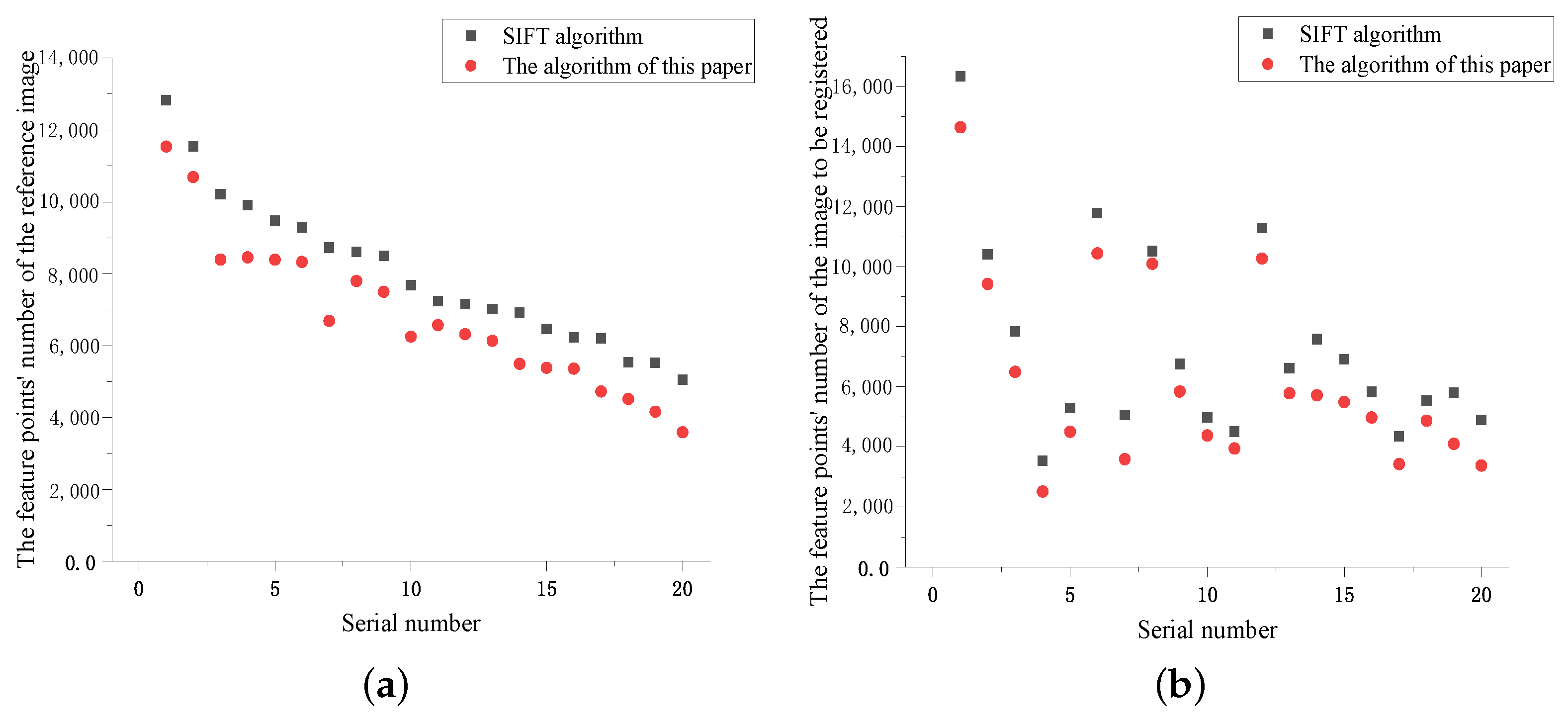
The specific experimental data of the Kitti dataset is displayed in

Table 1. Comparison of the results of Kitti dataset.

Number	SIFT Algorithm				The Algorithm of This Paper
	RN	WN	MN	PT(s)	rems	RN	WN	MN	PT(s)	rems
1	12,823	16,329	66	6.839	0.146	11,537	14,633	44	6.055	0.001
2	11,545	10,407	86	6.450	0.134	10,686	9419	54	5.817	0.131
3	10,204	7845	66	5.049	0.227	8387	6490	46	4.067	0.132
4	9909	3540	71	4.490	0.204	8452	2509	45	3.627	0.065
5	9486	5295	90	4.344	0.161	8390	4505	63	3.678	0.122
6	9276	11,774	71	5.346	0.384	8326	10,443	48	5.102	0.154
7	8725	5057	69	4.244	0.192	6689	3589	48	3.216	0.129
8	8604	10,518	83	4.850	0.147	7797	10,094	60	4.069	0.118
9	8497	6751	66	4.244	0.199	7497	5837	46	3.520	0.071
10	7674	4971	80	3.994	2.465	6251	4376	57	3.545	0.152
11	7240	4507	71	3.635	0.176	6567	3947	45	3.115	0.0.131
12	7152	11,281	65	4.014	0.517	6318	10,269	45	3.495	0.015
13	7011	6622	78	3.949	0.119	6136	5778	53	3.615	0.134
14	6914	7581	72	3.701	0.130	5391	5716	54	2.938	0.103
15	6457	6914	65	3.748	0.028	5383	5491	45	2.859	0.103
16	6223	5830	72	3.521	0.145	4355	4976	52	2.940	0.143
17	6203	4348	74	3.283	0.153	4725	3429	53	2.629	0.121
18	5538	5531	79	3.205	0.142	4514	4871	58	2.452	0.114
19	5520	5799	80	3.304	0.150	4159	4102	57	2.225	0.108
20	5057	4900	65	2.710	0.145	3589	3381	47	1.911	0.128

, and Figure 7 is a comparison diagram of the corresponding experimental results. Figure 7a,b, shows that the algorithm in this paper increased the stability factor when constructing the scale space compared with the SIFT algorithm. Feature points were fewer and more robust, and the algorithm running time was reduced, as shown in Figure 7c. The accuracy of image matching increased and the error decreased, as shown in Figure 7d, proving the superiority of this algorithm over the SIFT.

4.2.2. Comparison of Experimental Results Based on the Euroc Dataset

To avoid the contingency of the experiment, the Euroc dataset was also used to verify the algorithm in this paper. One group was randomly selected from the 20 groups of images in the dataset for display. The feature point extraction result of the reference image and of the image to be compared are shown in Figure 8 and Figure 9. After the optimization of the algorithm in this paper, the number of feature points of the reference image was reduced from 4649 to 3662, and the number of points decreased from 4308 to 3383. The matching results are shown in Figure 10. The running time of the SIFT algorithm corresponding to Figure 10a is 4.354 s; the running time of the algorithm in Figure 10b was 3.224 s, a reduction of 26.0%. The rems error dropped from 0.071 to 0.057.

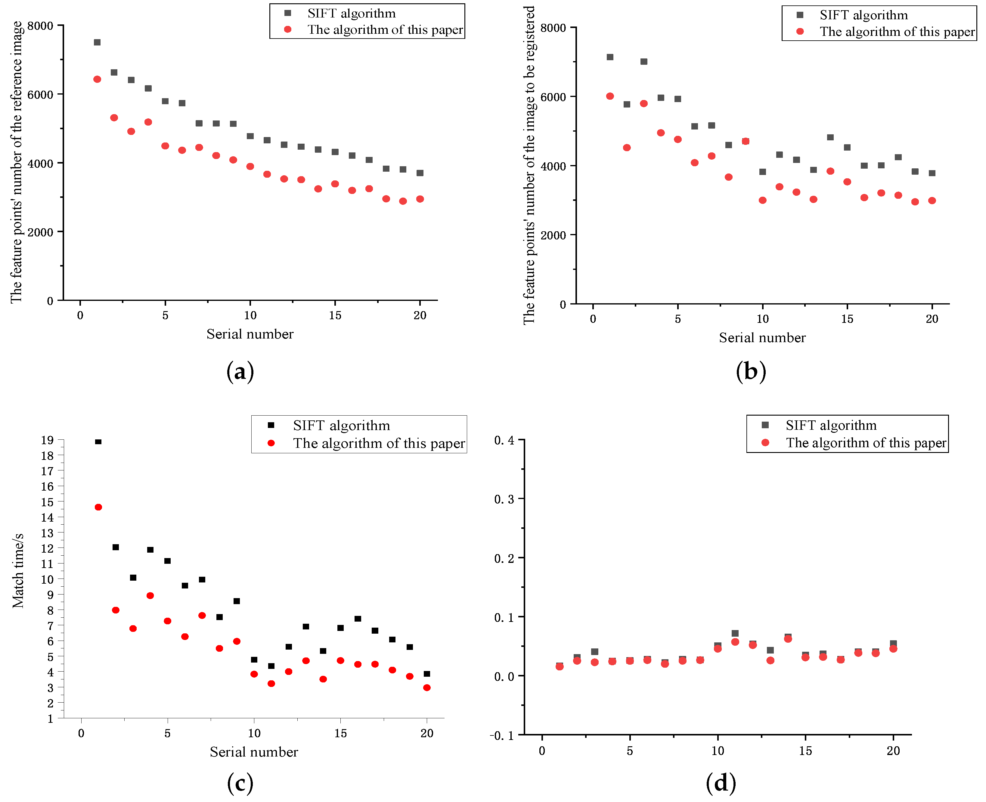
The specific experimental data of the kitti dataset is displayed in

Table 2. Comparison of the results of Euroc.

Number	SIFT Algorithm				The Algorithm of This Paper
	RN	WN	MN	PT(s)	rems	RN	WN	MN	PT(s)	rems
1	7497	7131	1132	18.869	0.016	6425	6005	1002	14.621	0.015
2	6623	5770	501	12.036	0.030	5307	4513	430	7.963	0.025
3	6400	7003	346	10.063	0.040	4908	5790	270	6.777	0.022
4	6156	5960	692	11.869	0.024	5178	4942	523	8.904	0.023
5	5784	5922	441	11.150	0.025	4485	4752	375	7.266	0.024
6	5729	5130	531	9.542	0.027	4360	4079	428	6.252	0.026
7	5141	5159	677	9.933	0.021	4441	4273	513	7.617	0.019
8	5138	4589	306	7.522	0.027	4206	3662	281	5.497	0.025
9	5130	4698	424	8.551	0.026	4079	4698	380	5.955	0.026
10	4774	3817	158	4.764	0.050	3891	2991	128	3.828	0.045
11	4649	4308	91	4.354	0.071	3662	3383	72	3.224	0.057
12	4518	4161	160	5.595	0.053	3529	3228	110	3.993	0.051
13	4463	3870	273	6.903	0.042	3505	3019	266	4.696	0.025
14	4382	4813	127	5.330	0.065	3238	3835	101	3.509	0.062
15	4308	4518	324	6.813	0.034	3193	3529	308	4.704	0.030
16	4204	3994	390	7.408	0.036	3243	3068	298	4.463	0.031
17	4081	4003	455	6.639	0.027	3243	3207	311	4.473	0.026
18	3826	4238	253	6.064	0.040	2947	3137	239	4.096	0.038
19	3802	3826	247	5.588	0.040	2879	2947	227	3.691	0.037
20	3697	3777	117	3.851	0.053	2941	2985	131	2.958	0.045

, and Figure 11 is a comparison diagram of the corresponding experimental results. Figure 11a,b compares the number of feature points of the reference image and the image to be compared. Compared with the SIFT algorithm, the number of feature points was greatly reduced, with an average reduction ratio of 20.4 and 19.3%, respectively. Figure 11c shows the comparison results of the image matching time, which was reduced on average by 30.0% compared with the SIFT algorithm; Figure 11d shows that the error comparison results of rems, decreased by 12.7%. The results on the Euroc dataset also demonstrated the advantages of our algorithm in matching time and error.

4.3. Comparison with Other Algorithms

To prove the advantage and significance of the algorithm proposed in this paper, this section compares its the experimental results with a state-of-the-art algorithm in the same dataset (three sets of datasets in Reference [36]). The comparison results are shown in Figure 12, Figure 13, Figure 14, Figure 15, Figure 16, Figure 17, Figure 18, Figure 19 and Figure 20.

Explanation of the meaning of the indicators in the

Table 3. Comparison of matching results of different affine distorted images.

Algorithm	MN	REMS	FT(s)	PT(s)	ST(s)
SIFT	479	$11.429$	$24.24$	$11.504$	$32.744$
Adaptive RKEM	245	$9.139$	$35.612$	$0.734$	$36.346$
This paper	166	$8.208$	$15.73$	$5.196$	$20.926$

,

Table 4. Comparison of matching results of images of different scales images.

Algorithm	MN	REMS	FT(s)	PT(s)	ST(s)
SIFT	263	$15.791$	$3.794$	$0.141$	$3.9235$
Adaptive RKEM	179	$9.139$	$6.172$	$0.020$	$6.192$
This paper	114	$8.486$	$2.443$	$0.019$	$2.462$

and

Table 5. Comparison of matching results of different illumination images.

Algorithm	MN	REMS	FT(s)	PT(s)	ST(s)
SIFT	361	$20.062$	$6.580$	$0.801$	$7.381$
Adaptive SIFT	228	$12.573$	$17.014$	$0.029$	$17.043$
This paper	184	$11.64$	$5.419$	$0.027$	$5.446$

: MN: number of matching points; FT: Feature extraction time (s); PT: match time; ST: total time.

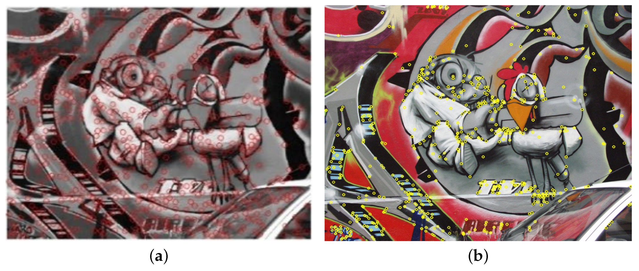
The first set is of images of different affine distortions. The detection results of the reference image feature points, the feature points of the image to be registered, and the image matching results from the adaptive SIFT algorithm and the algorithm in this paper are shown in Figure 12, Figure 13 and Figure 14. The specific data are shown in Table 3. It can be seen from the results that the algorithm in this paper had fewer matching points. The feature-point extraction and matching times as well as total time were all reduced.

The second set is of images of different scales. The detection results of reference image feature points and image feature points to be registered and the adaptive SIFT algorithm and the image matching results obtained by the algorithm in this paper are shown in Figure 15, Figure 16 and Figure 17. See Table 4 for specific data. It can be seen from the results that compared with the adaptive SIFT algorithm, the algorithm in this paper had fewer matching points, and the feature-point extraction and matching times were reduced as was total time.

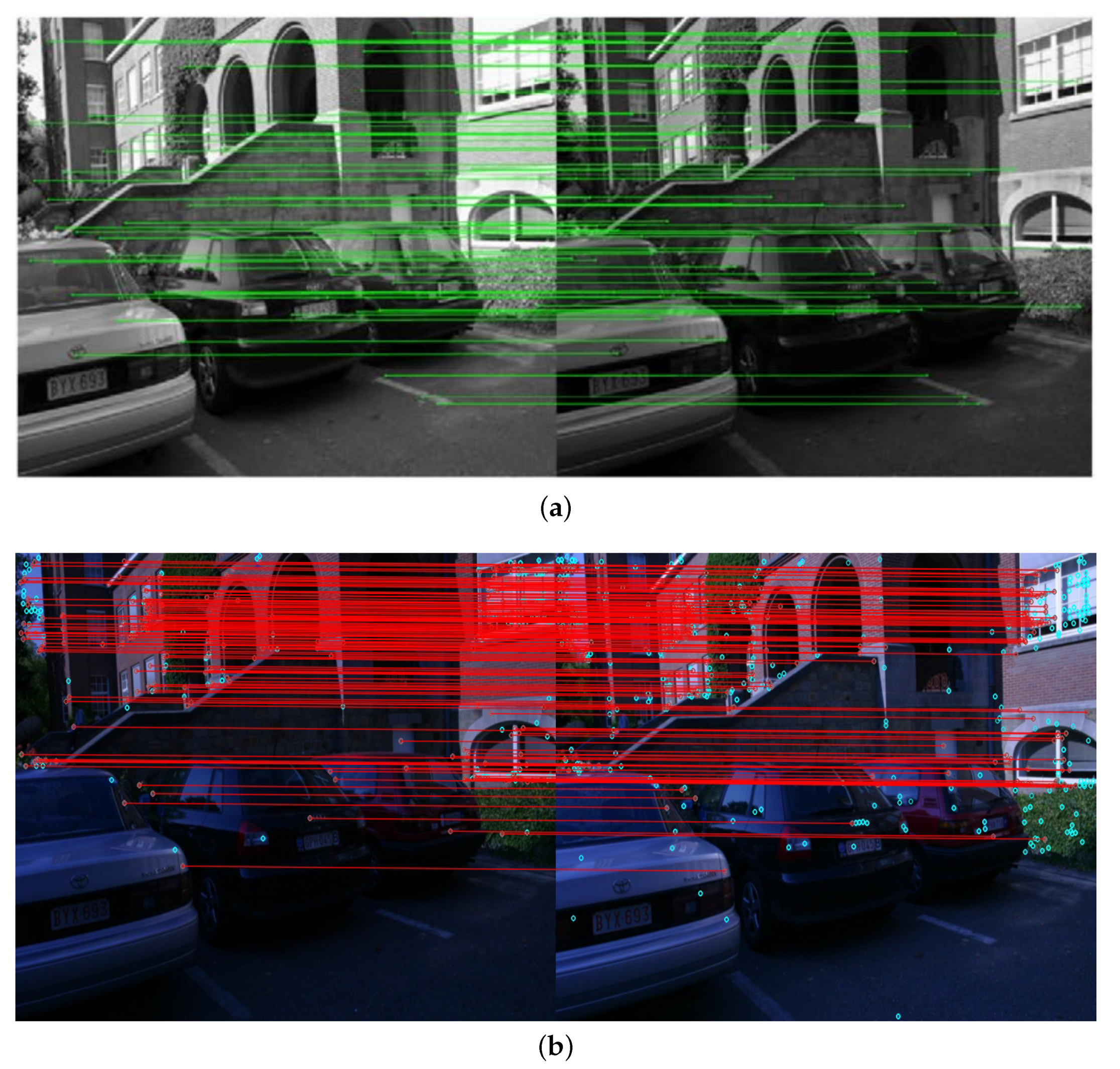
The third set is of images of different lighting. The detection results of reference image feature points and image feature points to be registered, and the image matching results obtained by the adaptive SIFT algorithm and the algorithm in this paper are shown in Figure 18, Figure 19 and Figure 20. See Table 5 for specific data. It can be seen from the results that the algorithm in this paper had fewer matching points, and the feature point extraction and matching times as well as total time were all reduced.

The three sets of data all show that the proposed algorithm had fewer matching points and less running time than the adaptive SIFT algorithm.

4.4. Summary of Experimental Results

To help readers intuitively feel the advantages of the algorithm in this paper, the index improvement of the algorithm compared with the SIFT algorithm and the adaptive SIFT algorithm is summarized, as shown in

Table 6. Comparison of matching results of different illumination images.

Dataset	PM	PT	REMS
Kitti dataset	$29.9\%$	$11.6\%$	$15.3\%$
Euroc dataset	$17.5\%$	$22.5\%$	$30.6\%$
Different affine distortion images	$32.2\%$	$18.8\%$	$10.2\%$
Different scale images	$36.3\%$	$5\%$	$7.1\%$
Different illumination images	$19.3\%$	$6.9\%$	$7.4\%$
Overall	$27.04\%$	$12.96\%$	$14.12\%$

.

5. Conclusions

To address the slow matching speed of the SIFT algorithm, this paper proposed a method of increasing the stability factor in the construction scale space, reducing the number of feature points and improving the stability of the feature points. According to the concept of reducing the time dimension, the four corners of the square description area of the SIFT feature point neighborhood were removed so that the dimension of the feature vector would be reduced, the operation speed accelerated, and the matching efficiency of the feature descriptor improved. To prove the effects and advantages of the algorithm, it was verified by the kitti and Euroc datasets. Then the algorithm was compared with a state-of-the-art algorithm. The results showed that the algorithm in this paper reduced the number of matching points for feature extraction time, matching time, and rems error by 27.04, 12.96, and 14.12%, respectively.

References

- Ma, J.; Jiang, X.; Fan, A.; Jiang, J.; Yan, J. Image matching from handcrafted to deep features: A survey. Int. J. Comput. Vis. 2021, 129, 23–79. [Google Scholar] [CrossRef]
- Jiang, X.; Ma, J.; Xiao, G.; Shao, Z.; Guo, X. A review of multimodal image matching: Methods and applications. Inf. Fusion 2021, 73, 22–71. [Google Scholar] [CrossRef]
- Li, C.; Yu, L.; Fei, S. Large-scale, real-time 3D scene reconstruction using visual and IMU sensors. IEEE Sens. J. 2020, 20, 5597–5605. [Google Scholar] [CrossRef]
- Ciaparrone, G.; Sánchez, F.L.; Tabik, S.; Troiano, L.; Tagliaferri, R.; Herrera, F. Deep learning in video multi-object tracking: A survey. Neurocomputing 2020, 381, 61–88. [Google Scholar] [CrossRef]
- Kechagias-Stamatis, O.; Aouf, N. Automatic target recognition on synthetic aperture radar imagery: A survey. IEEE Aerosp. Electron. Syst. Mag. 2021, 36, 56–81. [Google Scholar] [CrossRef]
- Wang, M.; Li, H.; Tao, D.C.; Lu, K.; Wu, X.D. Multimodal graph-based reranking for web image search. IEEE Trans. Image Process. 2012, 21, 4649–4661. [Google Scholar] [CrossRef]
- Wang, M.; Yang, K.Y.; Hua, X.S.; Zhang, H.J. Towards a rele-vant and diverse search of social images. IEEE Trans. Multimed. 2010, 12, 829–842. [Google Scholar] [CrossRef]
- Li, J.; Allinson, N.M. A comprehensive review of current local features for computer vision. Neurocomputing 2008, 71, 1771–1787. [Google Scholar] [CrossRef]
- Erxue, C.; Zengyuan, L.; Xin, T.; Shiming, L. Application of scale invariant feature transformation to SAR imagery registration. Acta Autom. Sin. 2008, 34, 861–868. [Google Scholar]
- Yan, Z.; Dong, C.; Wei, W.; Jianda, H.; Yuechao, W. Status and development of natural scene understanding for vision-based outdoor mobile robot. Acta Autom. Sin. 2010, 36, 1–11. [Google Scholar]
- Haifeng, L.; Yufeng, M.; Tao, S. Research on object tracking algorithm based on SIFT. Acta Autom. Sin. 2010, 36, 1204–1208. [Google Scholar]
- Lowe, D.G. Distinctive image features from scale-invariant keypoints. Int. J. Comput. Vis. 2004, 60, 91–110. [Google Scholar] [CrossRef]
- Ooi, B.C.; McDonell, K.J.; Sacks-Davis, R. Spatial Kd-tree: An indexing mechanism for spatial databases. In Proceedings of the IEEE International Computers Software and Applications Conference, Tokyo, Japan, 7–9 October 1987. [Google Scholar]
- Weinberger, K.Q.; Saul, L.K. Distance Metric Learning for Large Margin Nearest Neighbor Classification. J. Mach. Learn. Res. 2009, 10, 207–244. [Google Scholar]
- Chen, J.H.; Chen, C.S.; Chen, Y.S. Fast algorithm for robust template matching with M-estimators. IEEE Trans. Signal Process. 2003, 51, 230–243. [Google Scholar] [CrossRef]
- Torr, P.H.S.; Zisserman, A. MLESAC: A new robust estimator with application to estimating image geometry. Comput. Vis. Image Underst. 2000, 78, 138–156. [Google Scholar] [CrossRef]
- Choi, S.; Kim, T.; Yu, W. Performance evaluation of RANSAC family. In Proceedings of the British Machine Vision Conference, London, UK, 7–10 September 2009. [Google Scholar]
- Yan, K.; Sukthankar, R. PCA-SIFT: A more distinctive representation for local image descriptors. In Proceedings of the IEEE Conference on Computer Vision and Pattern Recognition, Washington, DC, USA, 27 June–2 July 2004. [Google Scholar]
- Mikolajczyk, K.; Schmid, C. A performance evaluation of local descriptors. IEEE Trans. Pattern Anal. Mach. Intell. 2005, 27, 1615–1630. [Google Scholar] [CrossRef]
- Lazebnik, S.; Schmid, C.; Ponce, J. A sparse texture representation using local affine regions. IEEE Trans. Pattern Anal. Mach. Intell. 2005, 27, 1265–1278. [Google Scholar] [CrossRef]
- Bay, H.; Tuytelaars, T.; Gool, L.V. SURF: Speeded up robust features. In Proceedings of the 9th European Conference on Computer Vision, Graz, Austria, 7–13 May 2006. [Google Scholar]
- Ojala, T.; Pietikainen, M.; Maenpaa, T. Multiresolution grayscale and rotation invariant texture classification with local binary patterns. IEEE Trans. Pattern Anal. Mach. Intell. 2002, 24, 971–987. [Google Scholar] [CrossRef]
- Ahonen, T.; Hadid, A.; Pietiainen, M. Face description with local binary patterns: Application to face recognition. IEEE Trans. Pattern Anal. Mach. Intell. 2006, 28, 2037–2041. [Google Scholar] [CrossRef]
- Jian, X.; Xiaoqing, D.; Shengjin, W.; Youshou, W. Background subtraction based on a combination of local texture and color. Acta Autom. Sin. 2009, 35, 1145–1150. [Google Scholar]
- Huang, D.; Ardabilian, M.; Wang, Y.H.; Chen, L.M. Asymmetric 3D/2D face recognition based on LBP facial representation and canonical correlation analysis. In Proceedings of the 16th International Conference on Image Procesing, Cairo, Egypt, 7–10 November 2009. [Google Scholar]
- Guo, Z.H.; Zhang, L.; Zhang, D.; Mou, X.Q. Hierarchical multiscale LBP for face and palmprint recognition. In Proceedings of the 16th International Conference on Image Procesing, Hong Kong, China, 26–29 September 2010. [Google Scholar]
- Guo, Z.H.; Zhang, L.; Zhang, D. A completed modeling of local binary pattern operator for texture classification. IEEE Trans. Image Process. 2010, 19, 1657–1663. [Google Scholar] [PubMed]
- Heikkila, M.; Pietikainen, M.; Schmid, C. Description of interest regions with local binary patterns. Pattern Recognit. 2009, 42, 425–436. [Google Scholar] [CrossRef]
- Tan, X.Y.; Triggs, B. Enhanced local texture feature sets for face recognition under difficult lighting conditions. IEEE Trans. Image Process. 2010, 19, 1635–1650. [Google Scholar] [PubMed]
- Mikolajczyk, K.; Schmid, C. A performance evaluation of local descriptors. In Proceedings of the International Conference on Computer Vision and Pattern Recognition, Madison, WI, USA, 18–20 June 2003. [Google Scholar]
- Abdel Hakim, A.E.; Farag, A.A. CSIFT: A SIFT descriptor with color invariant characteristics. In Proceedings of the International Conferenceon Computer Vision and Pattern Recognition, New York, NY, USA, 17–22 June 2006. [Google Scholar]
- Morel, J.M.; Yu, G. ASIFT: A new framework for fully affine invariant image comparison. SIAM J. Imaging Sci. 2009, 2, 438–469. [Google Scholar] [CrossRef]
- Li, L.; Fuyuan, P.; Kun, Z. Simplified SIFT algorithm for fast image matching. Infrared Laser Eng. 2008, 37, 181–184. [Google Scholar]
- Cai, G.R.; Li, S.; Wu, Y.; Su, S.; Chen, S. A perspective invariant image matching algorithm. Acta Autom. Sin. 2013, 39, 1053–1061. [Google Scholar] [CrossRef]
- Yonghe, T.; Huanzhang, L.; Moufa, H. Local feature description algorithm based on Laplacian. Opt. Precis. Eng. 2011, 19, 2999–3006. [Google Scholar]
- Hossein-Nejad, Z.; Agahi, H.; Mahmoodzadeh, A. Image matching based on the adaptive redundant keypoint elimination method in the SIFT algorithm. Pattern Anal. Appl. 2021, 24, 669–683. [Google Scholar] [CrossRef]
Figure 1.
Spatial extremum detection.
Figure 2.
Depiction of the 128-dimensional feature descriptor.
Figure 3.
96-dimensional feature descriptor.
Figure 4.
The extraction result of feature points of the 17th reference image. (a) Feature point extraction result of the SIFT algorithm; (b) feature point extraction result of this algorithm.
Figure 5.
Extraction results of feature points of the 17th group of images to be registered. (a) Feature point extraction result of the SIFT algorithm; (b) feature point extraction result of this algorithm.
Figure 6.
Matching results of the 17th group of pictures. (a) The matching results of the SIFT algorithm; (b) the matching results of the algorithm in this paper.
Figure 7.
Comparison of the kitti dataset’s specific experimental data in four categories. (a) the number of feature points of the reference image; (b) the number of feature points of the images to be compared; (c) matching time; (d) Rems errors.
Figure 8.
The extraction result of feature points of the 11th reference image. (a) Feature point extraction result of the SIFT algorithm; (b) feature point extraction result of this algorithm.
Figure 9.
Extraction results of feature points of the 11th group of images to be registered. (a) Feature point extraction result of the SIFT algorithm; (b) feature point extraction result of this algorithm.
Figure 10.
The matching results of the 11th group of pictures. (a) The matching results of the SIFT algorithm; (b) the matching results of the algorithm in this paper.
Figure 11.
Comparison of the Euroc dataset’s specific experimental data in four caegories: (a) the number of feature points of the reference image; (b) the number of feature points of the images to be compared; (c) matching time; and (d) Rems errors.
Figure 12.
The extraction result of feature points of the reference image. (a) The extraction result of the adaptive RKEM algorithm; (b) the extraction result of the algorithm in this paper.
Figure 13.
The extraction result of feature points of the image to be registered. (a) The adaptive RKEM algorithm; (b) The extraction result of the algorithm in this paper.
Figure 14.
Matching results of images with different affine distortions. (a) The adaptive RKEM algorithm; (b) The algorithm in this paper.
Figure 15.
Extraction result of feature points of the reference image. (a) The adaptive RKEM algorithm; (b) The algorithm in this paper.
Figure 16.
The extraction result of feature points of the image to be registered. (a) The adaptive RKEM algorithm; (b) The algorithm in this paper.
Figure 17.
Matching results of images with different affine distortion. (a) The adaptive RKEM algorithm; (b) The algorithm in this paper.
Figure 18.
The extraction result of feature points of the reference image. (a) the adaptive RKEM algorithm; (b) the algorithm in this paper.
Figure 19.
Figure 20.