
Fault Diagnosis Method for Rolling Bearings Based on Two-Channel CNN under Unbalanced Datasets


College of Coastal Defense Force, Naval Aviation University, Yantai 264001, China
*
Author to whom correspondence should be addressed.
Appl. Sci. 2022, 12(17), 8474; https://0-doi-org.brum.beds.ac.uk/10.3390/app12178474
Submission received: 26 July 2022
/
Revised: 18 August 2022
/
Accepted: 22 August 2022
/
Published: 25 August 2022
(This article belongs to the Collection Bearing Fault Detection and Diagnosis)
Abstract
:As a critical component in industrial systems, timely and accurate fault diagnosis of rolling bearings is closely related to reliability and safety. Since the equipment usually operates in normal conditions with few fault samples, unbalanced data distribution problems lead to poor fault diagnosis ability. To address the above problems, a two-channel convolutional neural network (TC-CNN) model is proposed. Firstly, the frequency spectrum of the vibration signal is extracted using the Fast Fourier Transform (FFT), and the frequency spectrum is used as the input to the one-dimensional convolutional neural network (1D-CNN). Secondly, the time-frequency image of the vibration signal is extracted using generalized S-transform (GST), and the time-frequency image is used as the input to the two-dimensional convolutional neural network (2D-CNN). Then, feature extraction in the convolution and pooling layers is performed in the above two CNN channels, respectively. The feature vectors obtained from the two CNN models are stitched together in the fusion layer, and the fault classes are identified using an SVM classifier. Finally, using the rolling bearing experimental dataset of Case Western Reserve University (CWRU), the fault diagnosis effect of the proposed TC-CNN model under various data imbalance conditions is verified. In comparison with other related works, the experimental results demonstrate the better fault diagnosis results and robustness of the method.
1. Introduction
In modern industries, machinery is more complex and intelligent, and many sensors are installed in the system to detect the health condition of the equipment. These sensors collect a large amount of system operation data. Intelligent fault diagnosis algorithms can explore the in-depth features and apply them to fault diagnosis, and scholars have achieved many results for data-driven fault diagnosis methods [1,2,3]. Most of the failures of rotating machinery systems are due to the failure of rolling bearings. Failure of rolling bearings can affect system operation, which leads to economic loss and time wastage. Therefore, the reliability and safety of rolling bearings are crucial for the whole equipment. The fault diagnosis problem of rolling bearings needs more extensive research [4,5,6,7,8,9,10].
Deep belief network (DBN) [11], auto-encoder (AE) [12], CNN [13], etc. intelligent fault diagnosis algorithms have been rapidly developed [14,15]. He et al. used a genetic algorithm-optimized DBN to diagnose gear transmission chain faults [11]. Gu et al. constructed a deep neural network (DNN) based on multiple AEs, and directly input the time domain vibration signal into the DNN for feature learning and fault diagnosis [16]. This method only extracts time domain features and does not consider the features of other domains, so it does not fully utilize the features of the signals. Saucedo-Dorantes et al. designed a rolling bearing fault diagnosis model consisting of multiple stacked auto-encoders (SAE) [17]. Multiple SAEs are used to extract the time domain, frequency domain, and time-frequency domain features of the signal simultaneously, and then the features from different domains are combined. This method is better than the PCA+neural network (NN) and LDA+NN. Compared with AE and DBN, CNN are more advantageous in processing time series data and images [18]. In recent years, researchers have used CNN to extract discriminative features directly. Levent combined the feature extraction and classification stages of CNN to reduce the computational complexity [19]. Pan et al. combined CNN with the second-generation wavelet transform to enhance the robustness of fault diagnosis [20]. Qiao et al. enhanced the sensitivity of CNN to fault features through an adaptive weight vector [21]. Peng et al. converted the vibration signal of the rolling bearing into a grayscale image, used the grayscale image to extract fault features, and achieved a better fault diagnosis result [22].
Although all of the above CNN models achieve good diagnostic results, these methods are premised on balanced datasets. However, in the actual working condition, rolling bearings have faults occur infrequently, resulting in insufficient failure data compared to normal data, thus affecting the fault diagnosis accuracy and stability [23]. The imbalanced data make the features learned by CNN more biased to normal state sample features and under-fit to fault sample. The common idea is to compose a balanced dataset by increasing the number of faulty samples, thus eliminating the adverse effects of imbalance learning. Chawla et al. proposed the synthetic minority oversampling technique (SMOTE) to randomly generate virtual samples to balance the training set [24]. Tang et al. used a Wasserstein generative adversarial network (WGAN) to balance training samples and reduce differences in fault data distribution [25]. Wang et al. used GAN to generate new samples and diagnosed faults by superposition denoising auto-encoder (SDAE) [26]. Mao et al. applied the fast Fourier transform (FFT) to preprocess the acquired data and generate synthetic minority class samples using GAN [27]. Xuan et al. proposed a multi-view GAN (MV-GAN) to extend the image dataset automatically [28]. Li et al. used GAN to generate empirical mode decomposition (EMD) energy spectrum data, and the fault diagnosis results were better than traditional oversampling techniques [29]. Han et al. combined adversarial learning with CNN to improve the robustness [30]. Akhenia et al. used multiple time-frequency feature extraction methods to extract two-dimensional time spectrum images from bearing fault signals and then used single image GAN (SinGAN) to generate additional datasets [31]. Tong et al. used auxiliary classifier GAN with spectral normalization (ACGAN-SN) for bearing fault detection. The experimental results proved that ACGAN-SN has better stability than GAN [32]. Ruan et al. modified the GAN generator based on the fault diagnosis results of CNN. In addition, the envelope spectrum error is taken as another correction term, so that fault samples can contain more information [33]. Although all the above methods can solve the fault diagnosis problem under unbalanced datasets to some extent, the following problems exist: generating new samples will change the distribution of the original data, which tends to increase the training time as well as lose important sample information, meaningless noise data may be generated when the data are extremely unbalanced, and the reliability of fault diagnosis results based on noise data are poor. Furthermore, the availability of generated data is related to the adequacy of the initial data. Due to the infrequent occurrence of faults, limited fault data are obtained. Learning trends and characteristics of fault data can be challenging if the initial fault data are insufficient.
This paper proposed a TC-CNN model to address the above problems. The TC-CNN model discovers more information by simultaneously extracting fault features in the frequency domain and time-frequency domain of the vibration signal. Feature discovery engineering is the focus of fault diagnosis. As long as the separability of data features is good enough, it is easy to obtain good results no matter how strong the data imbalance is. Adding fault features or making them easier to learn is another effective way to solve problems. Compared with the DAE model proposed in [16], the proposed method can simultaneously extract fault features in two feature domains and reduce the difficulty of fault diagnosis by increasing the dimension of features [17] used EMD for feature extraction, and time-frequency features were expressed as a set of intrinsic pattern functions (IMFs). The difference of the proposed method is that: GST is used to extract time-frequency features and represent them in the form of images, which takes advantage of the convolutional structure of CNN in image feature extraction. Summarizng the main contributions of this paper: (1) A TC-CNN model based on 1D-CNN and 2D-CNN is proposed, which increases the dimensionality of extracted features by extracting features in both the frequency domain and time-frequency domain. (2) FFT is used to extract the frequency spectrum as the input of 1D-CNN, and GST is used to extract the time-frequency image as the input of the 2D-CNN. (3) Feature extraction is carried out in two CNN channels, respectively. The splicing of the two feature vectors is performed in the fusion layer. The features learned from frequency spectrums and time-frequency images are fused and incorporated into the training and learning process of TC-CNN.
The rest of this article can be summarized as follows: Section 2 introduces the two feature extraction methods used in TC-CNN. Section 3 introduces the theory related to CNN, and the framework of the TC-CNN model is given. Section 4 verifies the performance of TC-CNN through several experiments. Moreover, the proposed TC-CNN model is compared with the approximate and existing models to show its advantages. Section 5 summarizes the limitations of the proposed method and future research priorities.
2. Feature Extraction Method
2.1. FFT
FFT is a common tool for signal processing and is widely used in feature extraction, radar signal processing, etc. The specific implementation is shown as follows.
For a finite-length discrete signal , , its discrete Fourier transform (DFT) can be expressed as:
where , . FFT decomposes into an even sequence and an odd sequence :
where and are both of length . In addition, then we can obtain:
The following formula can be obtained:
Because :
where and are the DFTs of and at , respectively. Since both and have a period of , can be expressed as:
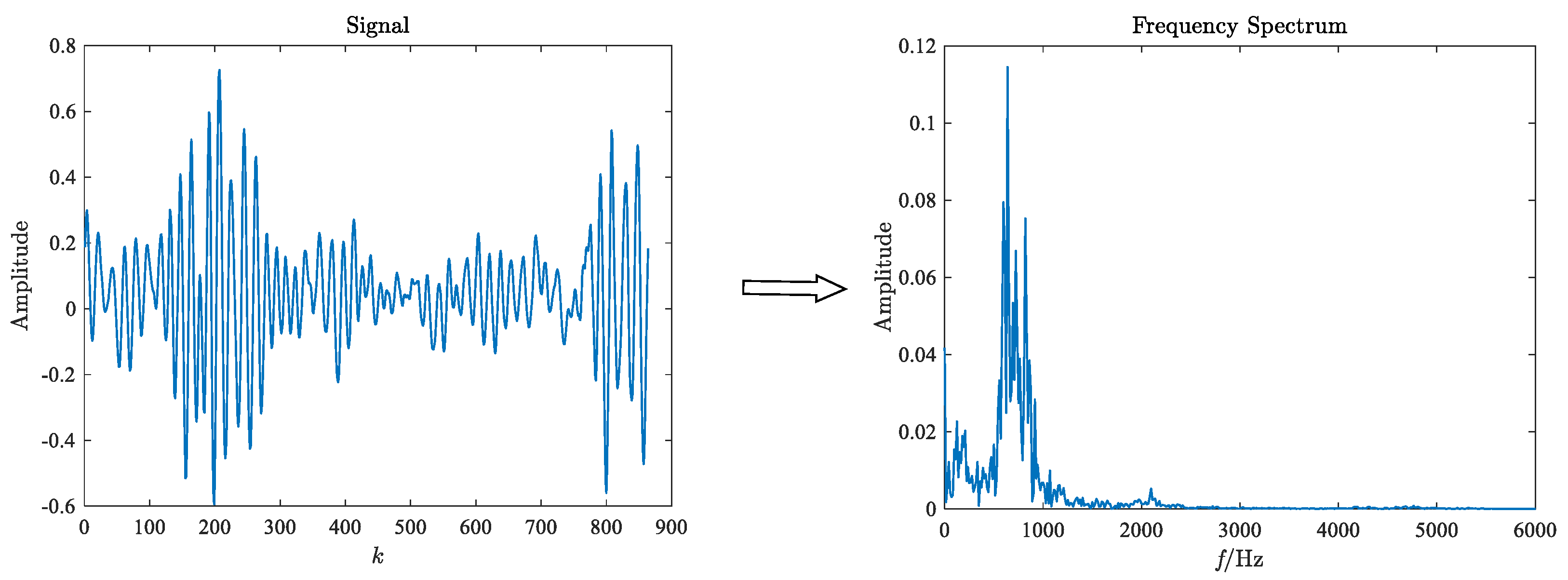
where . The frequency spectrum obtained by performing FFT on a signal is shown as follows.
2.2. GST
Vibrational signal analysis techniques such as EMD [34], Short time Fourier transform (STFT) [35], Wigner–Ville distribution (WVD) [36], and wavelet packet transform (WPT) [37] are widely used in fault diagnosis. Compared with GST, these methods have some shortcomings when used as deep learning inputs. For EMD because IMF is frequency independent, it is impossible to judge the correlation between fault characteristics and IMF, so IMFs have difficulty being unified as deep learning inputs. STFT obtains the time-frequency spectrum based on a sliding time window. When the window width is short, it has high time resolution and low frequency resolution. Once STFT determines the window function, the corresponding time-frequency resolution is also determined. For non-stationary signals, WVD is similar to STFT. WVD analyzes the time-frequency distribution of vibration signals. However, WVD has the problem of cross-interference in engineering applications, and unlike manual analysis, it is difficult for deep learning methods to distinguish cross-term interference automatically. WPT can decompose the high frequency parts compared to wavelet transform, which improves the resolution of a high frequency band. However, the characteristic frequency of bearing faults in rotating machinery is generally less than ten times that of the rotation frequency so WPT may increase computational cost. In conclusion, GST is chosen as the time-frequency domain feature extraction method, and the specific implementation method is described as follows.
The formula for the Fourier transform is:
Since the classical Fourier transform cannot locate both time and frequency, a window function can be introduced, then the formula for the Fourier transform is:
If the window function is a normalized Gaussian window function with scaling and translation, then the window function is:
The frequency spectrum of the signal is:
Because (10) is a function of three independent variables, it is not practical as a tool for time-frequency analysis. If is simplified to , then the S-transform is defined as:
The S-transform is the extension of the continuous wavelet transform (CWT). In (11), the window width is fixed, which means that the width of the time-frequency window has the same resolution for all frequency components. The test signals of rotating machines are generally non-stationary signals with many frequency components. The change is more violent in the high-frequency part, and the duration is relatively short. At this time, the time window should be taken narrower. On the contrary, the time window should be taken wider. Based on the above analysis, it is possible to relate the scale factor to the frequency. Let the scale factor become a function of the frequency f to adjust the width of the time window adaptively with frequency. Let , where . According to (10), the generalized S-transform can be obtained:
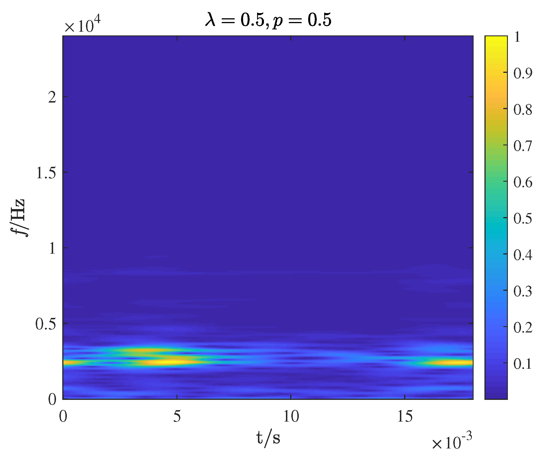
When , GST is the standard S-transform. The Gaussian window function can be chosen flexibly with the change of frequency scale, which makes the GST better adapted to the analysis and processing of different practical signals. In general, p should not be too large, although GST does not theoretically limit its value. Since p is very sensitive to the frequency change in the actual signal analysis, the value is too large to make the window function too narrow, which is unsuitable for the time-frequency analysis. On the other hand, when p gradually becomes small, the analysis result will be closer to STFT. When p is fixed, the modulation factor can adjust to increasing and decreasing curvature to the modulation effect caused by p. For the original signal in Figure 1, its GST time-frequency image is shown in Figure 2, where , the horizontal coordinate is time, and the vertical coordinate is frequency.
3. TC-CNN Model Framework
CNN has achieved excellent results in various fields with its feature extraction and pattern recognition capabilities, so CNN is used as a theoretical analysis tool. This section briefly introduces the principle of CNN first and then gives the rolling bearing fault diagnosis process using the TC-CNN model.
3.1. CNN
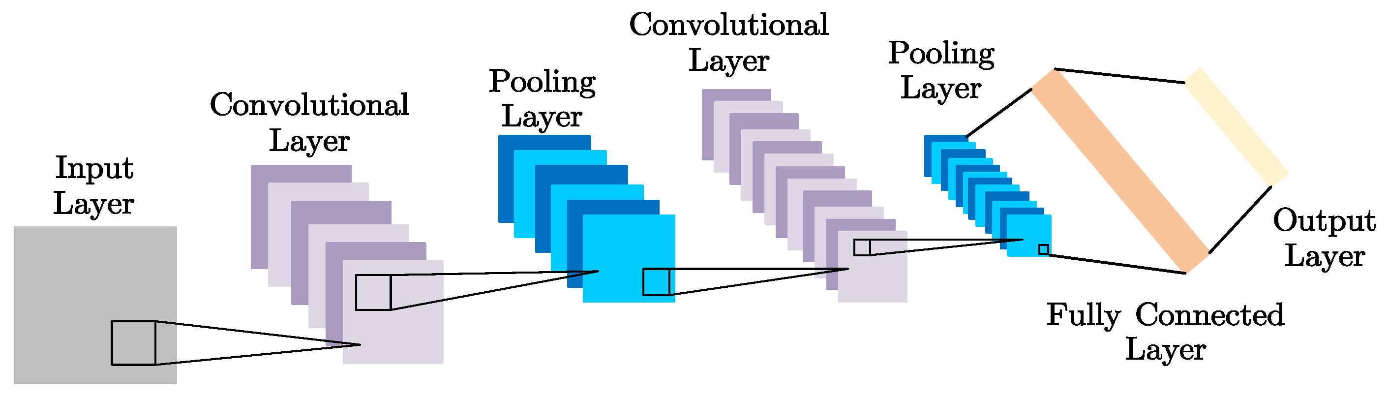
CNN consists of the input layer, the hidden layer, the fully connected layer, and the output layer [38]. The hidden layer is alternately composed of convolutional layers and pooling layers. The fully connected layer and the output layer form the classifier of CNN. The convolution layer is convolved with the feature map of the input layer by a convolution kernel, and the output feature is obtained through the activation function. The feature map is filtered in the pooling layer. A typical CNN structure is shown in Figure 3 [39].
3.1.1. Convolutional Layer
The convolution layer contains several convolution kernels. The feature maps or feature vectors from the previous layer are input to the convolutional layer, which are convolved with convolutional kernels and mapped with the activation function to the new feature information. CNN uses the following formula for convolution operation:
where l denotes the lth layer, is the feature matrix of the mth or previous layer input, is the weight matrix of the th convolution kernel, is the bias vector, is the feature matrix of the lth layer output, and f is the activation function.
3.1.2. Activation Function
The nonlinear activation function is an indispensable key module in CNN. In order to prevent the gradient explosion or gradient dispersion, the commonly used ReLU function is used in this paper:
3.1.3. Pooling Layer
CNN sets up a pooling layer to perform downsampling operations to simplify and refine the output feature information, reducing the dimension and capturing more feature information. CNN uses the following formula for pooling operation:
where is the output matrix, and S is the size of the pooling layer.
3.1.4. Fully Connected Layer
As the output layer of the network, the fully connected layer is the classifier, and its role is to map the feature information learned by the network to the label space of the samples. In this paper, SVM is used as the classifier. The extracted features are processed through SVM to achieve classification.
3.2. The Proposed TC-CNN Model
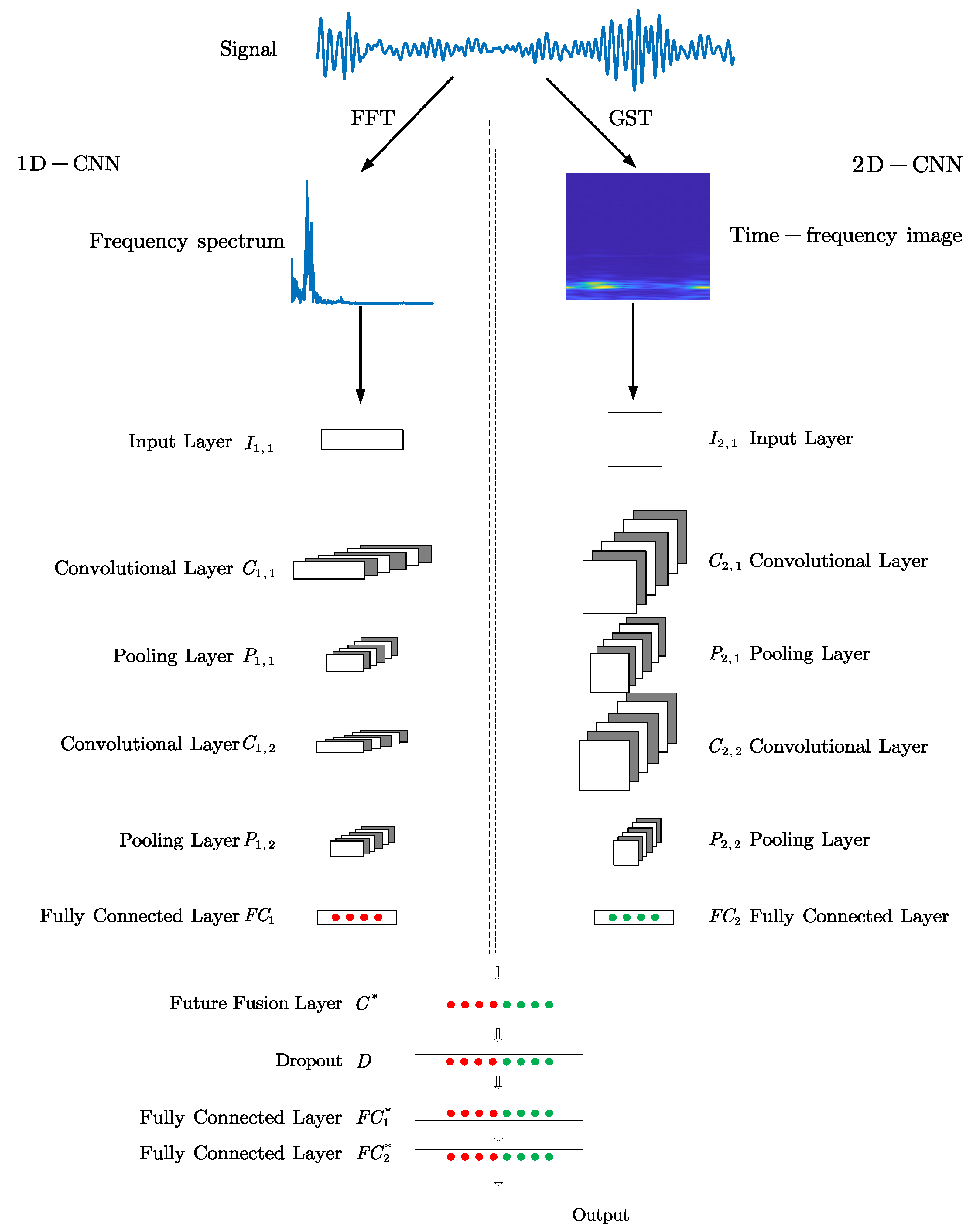
The proposed TC-CNN model combines FFT, GST, and CNN, and the flowchart of the proposed TC-CNN structure used to rolling bearing fault diagnosis is shown in Figure 4.
The parallel convolution structure of 1D-CNN and 2D-CNN is used for feature extraction. The model includes a 1D convolutional structure based on the frequency spectrum and a 2D convolutional structure based on the GST time-frequency image. The proposed method can fully utilize the sample fault information and make the fault information complement each other. Both CNN models have two convolutional layers, two pooling layers, and one fully connected layer. The features extracted by and are stitched by feature fusion layer . To improve the generalization ability, the Dropout operation is added between and .
The fault diagnosis process can be divided into four parts: (1) Firstly, frequency spectrums and GST time-frequency images are obtained by FFT and GST on the original sampled data. (2) The frequency spectrum and GST time-frequency image are input to the feature extractor for fault feature extraction and obtain the combined fault features by a feature fusion layer. (3) The convolutional network is used for supervised learning of combined fault features, and the weights and parameters in the model are trained and updated. (4) The fault classification performance of TC-CNN is verified through the fault dataset.
3.3. Evaluation Criterion
Accuracy is a common evaluation criterion in neural networks. However, the evaluation cannot be performed by accuracy alone if the dataset is unbalanced. The model will make the classification result favor the majority class during the training process so that the model has high accuracy. However, the classification result of minority class samples is more meaningful. High accuracy is not equivalent to a better classification result. Therefore, the F1 score is also used to measure the model more accurately and comprehensively in the paper. The basic form of the confusion matrix is given:
| Predicted | |||
| Actual | Positive | Negative | |
| Positive | True Positive (TP) | False Positive (FP) | |
| Negative | False Negative (FN) | True Negative (TN) | |
3.3.1. Accuracy
Accuracy is the percentage of correctly predicted outcomes over the total sample:
3.3.2. Precision
Precision is the probability of the sample that is True among all the samples that are predicted to be True:
3.3.3. Recall
Recall is the probability of a positive sample being predicted out of an actual positive sample:
3.3.4. F1 Score
The higher values of precision and recall are better. However, precision and recall may have one high value and another low value, so the F1 score is introduced to combine precision and recall. F1 score measures the ability to find positive samples:
For the multiclassification problem, this paper uses the macro F1 score calculation as follows:
where n is the total number of fault classes, is the F1 score of the class i, .
4. Experimental Analysis
4.1. Experimental Data
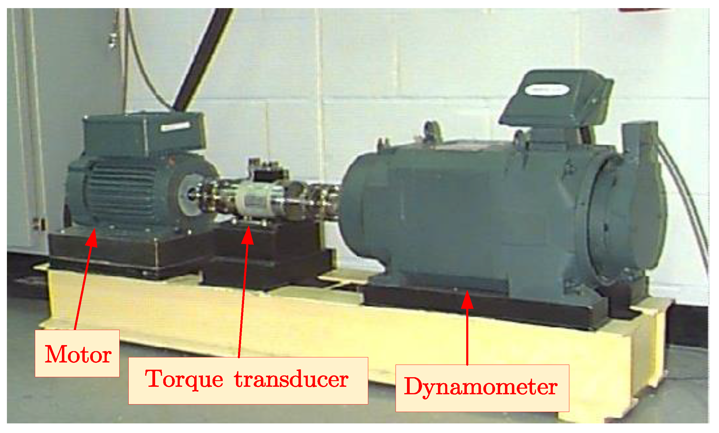
In this paper, the bearing fault dataset of CWRU is used to verify the performance of the TC-CNN fault diagnosis model [40]. The experimental facility is shown in Figure 5.
The main components of this experimental facility include a 2-hp motor (left), a torque transducer (middle), and a dynamometer (right). The test bearing (6205-2RS JEM SKF) supports the motor shaft. The signals are collected from the drive end bearing with a sample rate of 48,000 Hz, a motor load of 0 hp, and an average motor speed of 1724 rpm. The fault locations mainly included ball defects (BD), outer ring defects (OR), and inner ring defects (IR). Faults in this database of bearings are generated by electrical machining with fault sizes of 0.007 inches, 0.014 inches, and 0.021 inches. Each fault location has the above three damage conditions, representing different severity. Therefore, there are ten classes of data, and the information is listed in Table 1.
The symbol @6:00 in Table 1 indicates that the fault direction is at 6 o’clock.
4.2. Model Parameters
The paper is set with a sample of 1024 data points, , in GST: (1) The original test signal of dimension is performed FFT, and the dimension frequency spectrum is obtained. (2) The original test signal of dimension is compressed to a time-frequency image through GST. The purpose of compression is to highlight the primary feature information and not drown out other information, reduce the interference of background information, and improve the proportion of main features. The time-frequency image and frequency spectrum are the input of 2D-CNN and 1D-CNN, respectively. (3) The features extracted from the two CNN models are combined to obtain the final fault features. The network model parameters are obtained based on actual test results. The parameters set for the two networks are shown in Table 2.
The last fully connected layer is an SVM classifier, and the kernel function is Gaussian kernel. The kernel parameter , and the penalty factor . The remaining parameters are as follows: the dropout ratio is 0.5, the learning rate is 0.005, the mini-batch size is 8, the total epochs is 500, and the loss function is cross-entropy.
4.3. Fault Diagnosis Results under a Balanced Dataset
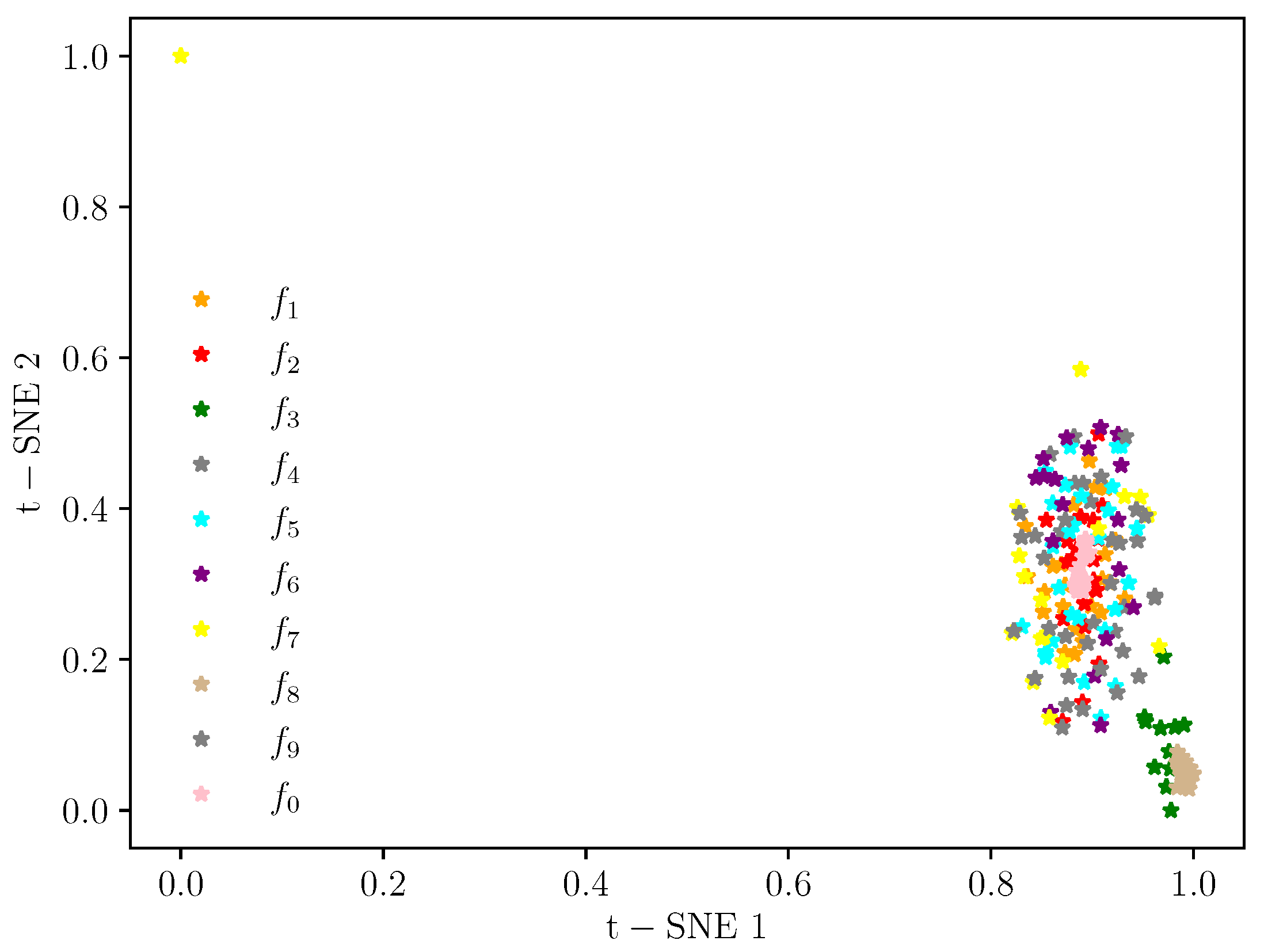
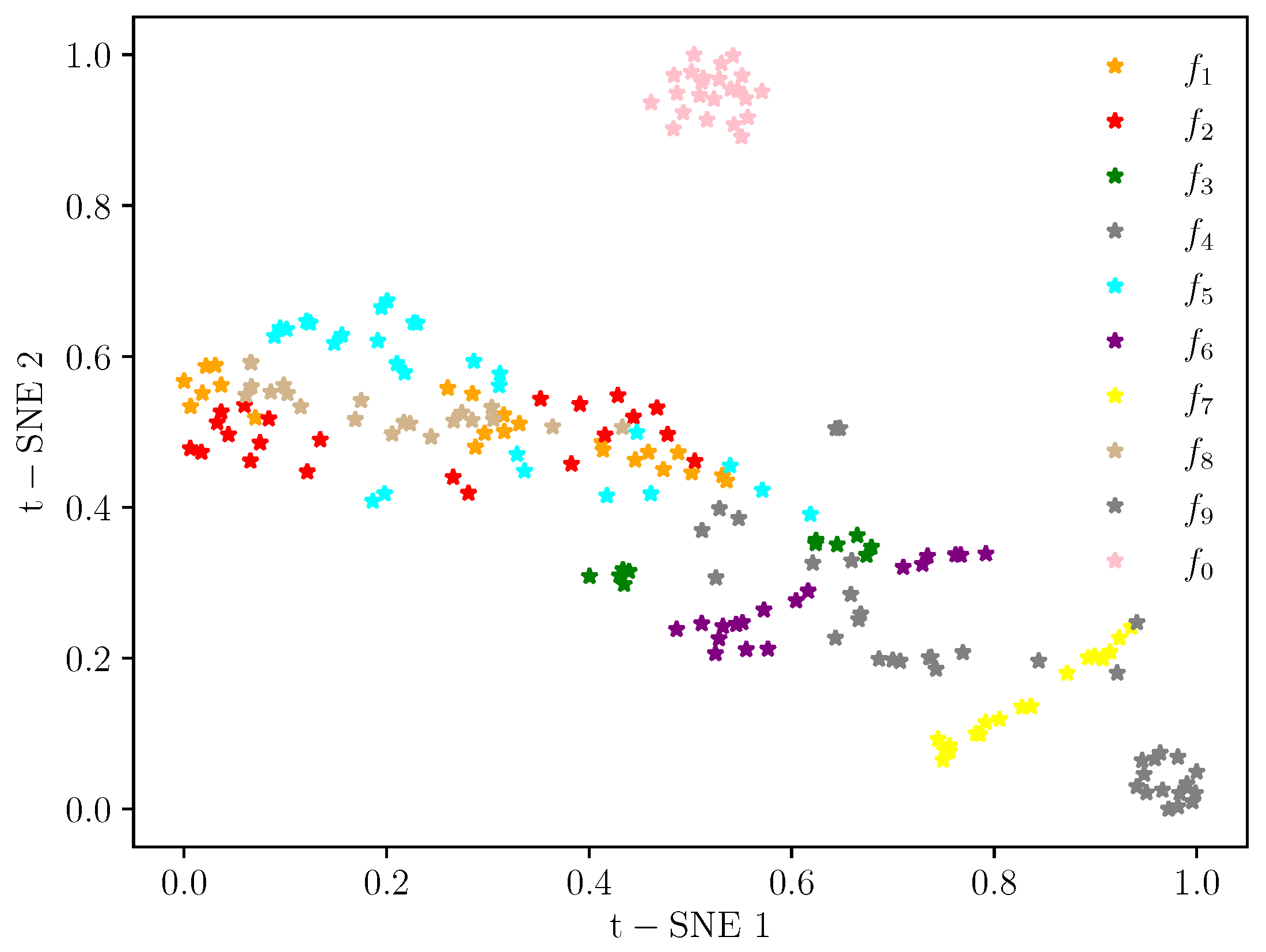
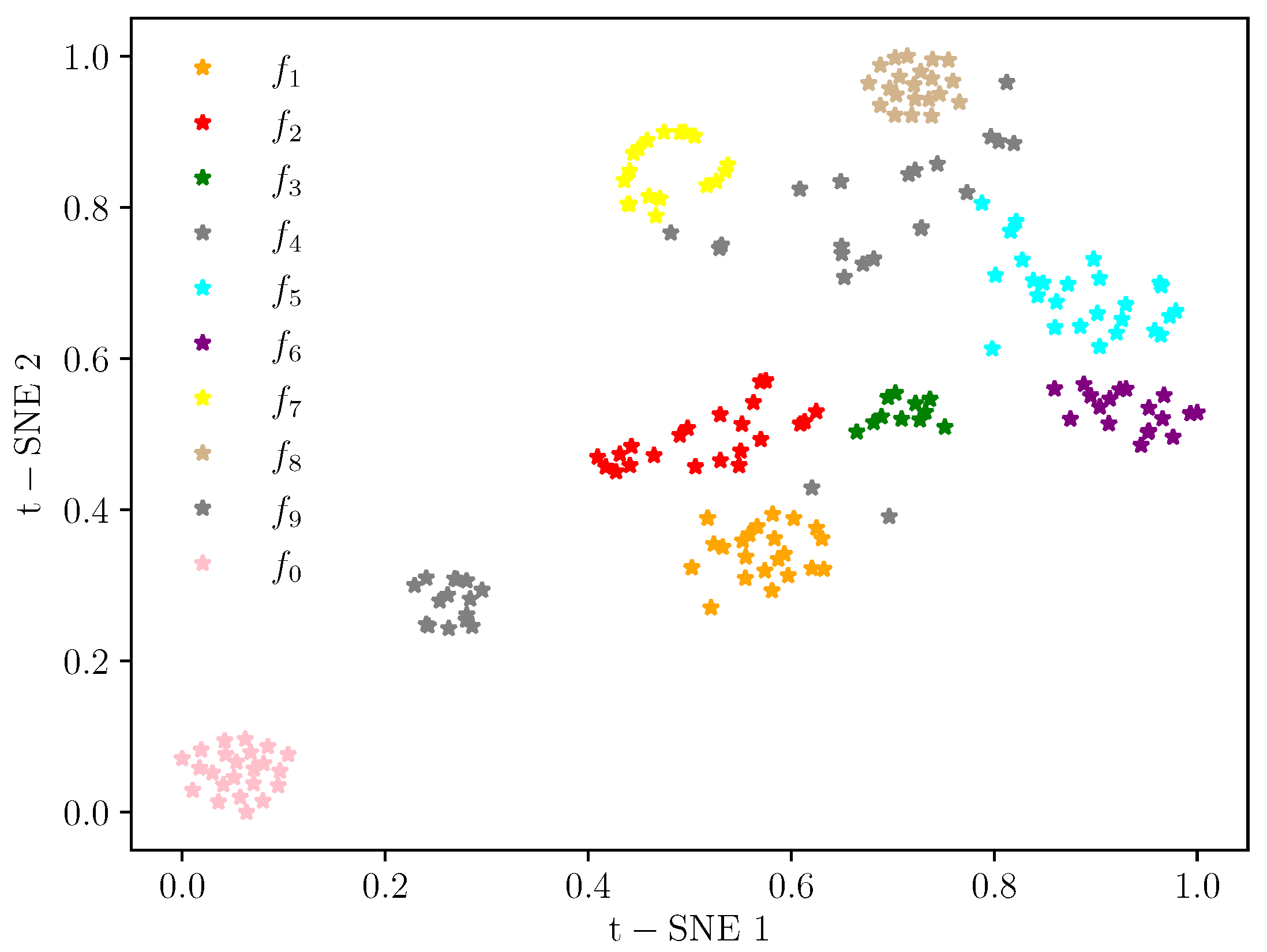
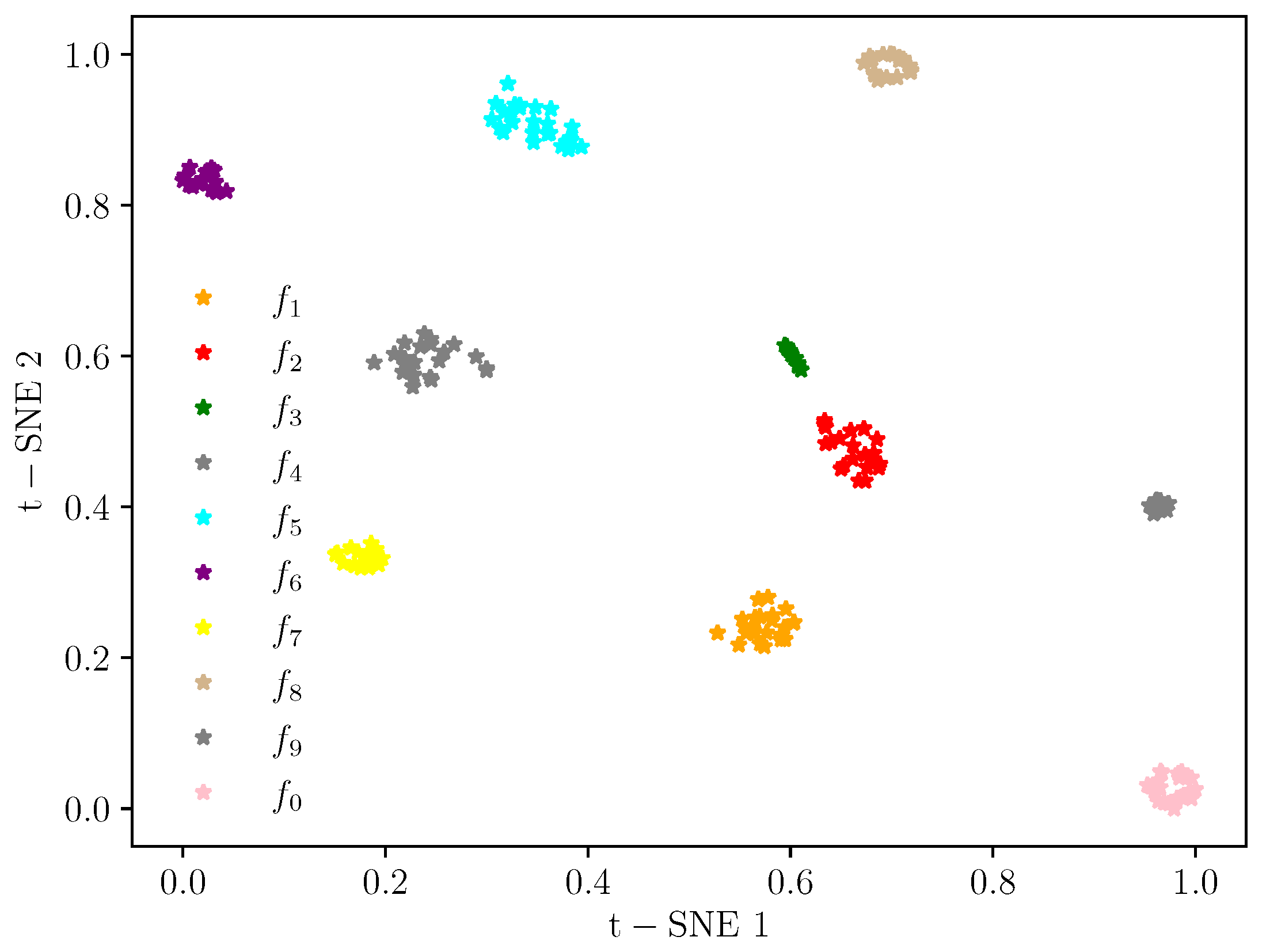
In addition, 200 samples are randomly constructed for each class, and a sample set containing 2000 samples is constructed. Visualize the hierarchical feature learning process of TC-CNN using the t-distributed Stochastic Neighbor Embedding (t-SNE) method [41]. The learned features of the original input signal, fully connected layers , and of the test dataset are mapped to two-dimensional features using t-SNE, respectively. The mapped features of different layers are shown in Figure 6, Figure 7, Figure 8 and Figure 9.
Figure 6, Figure 7, Figure 8 and Figure 9 show the feature map changes for different classes during the model learning process. As shown in Figure 6, the original data features for all classes are relatively scattered and difficult to distinguish. Figure 7 and Figure 8 show the learned features of the fully connected layers and , respectively. Compared with the original input data, it can be seen that, after the convolution and pooling operations, the samples are gradually clustered. Furthermore, the clustering of features in the fully connected layer is better than that in . Finally, in Figure 9, features of the same class are very concentrated. The distance between the feature distributions in is the largest compared to the feature mapping results in and . The classifier easily performs the classification of the dataset, illustrating the excellent classification results.
The proposed methods in this paper are compared with 1D-CNN, 2D-CNN [22], CWT+2D-CNN [38], DBN [42], and 1D-CNN+2D-CNN.
(1) 1D-CNN consists of an input layer, two 1D convolutional layers, two pooling layers, a fully connected layer, a softmax classifier, and an output layer. The kernel sizes of input and output channels of the convolutional and pooling layers are set as 5, 6, 3, and 6, respectively. The rest of the structural parameters are the same as the 1D-CNN in the proposed model.
(2) Since the dimension of the original signal data are 1024, the original signal data are transformed into a 32 × 32 dimensional matrix as the input of 2D-CNN. The classifier is softmax. The rest of the structural parameters are the same as the 2D-CNN in the proposed model.
(3) CWT+2D-CNN uses CWT to extract the time-frequency features, and the Morlet cmor3-3 wavelet basis function is selected. The CWT time-frequency image is used as the input of the 2D-CNN, and the classifier is softmax. The rest of the structural parameters are the same as the 2D-CNN in the proposed model.
(4) The DBN contains an input layer, two hidden layers, and one output layer, and the network structure is [1024, 50, 20, 10]. The learning rate is 0.05, a mini-batch size is 8, and the number of iterations is 500.
(5) 1D-CNN+2D-CNN has the same network structure as TC-CNN. The difference is that TC-CNN uses FFT and GST to extract features. The inputs of the two channels are frequency spectrum and time-frequency images, respectively. In the 1D-CNN+2D-CNN, the inputs of the two channels are the original signal and the 2D matrix transformed into the original signal, respectively.
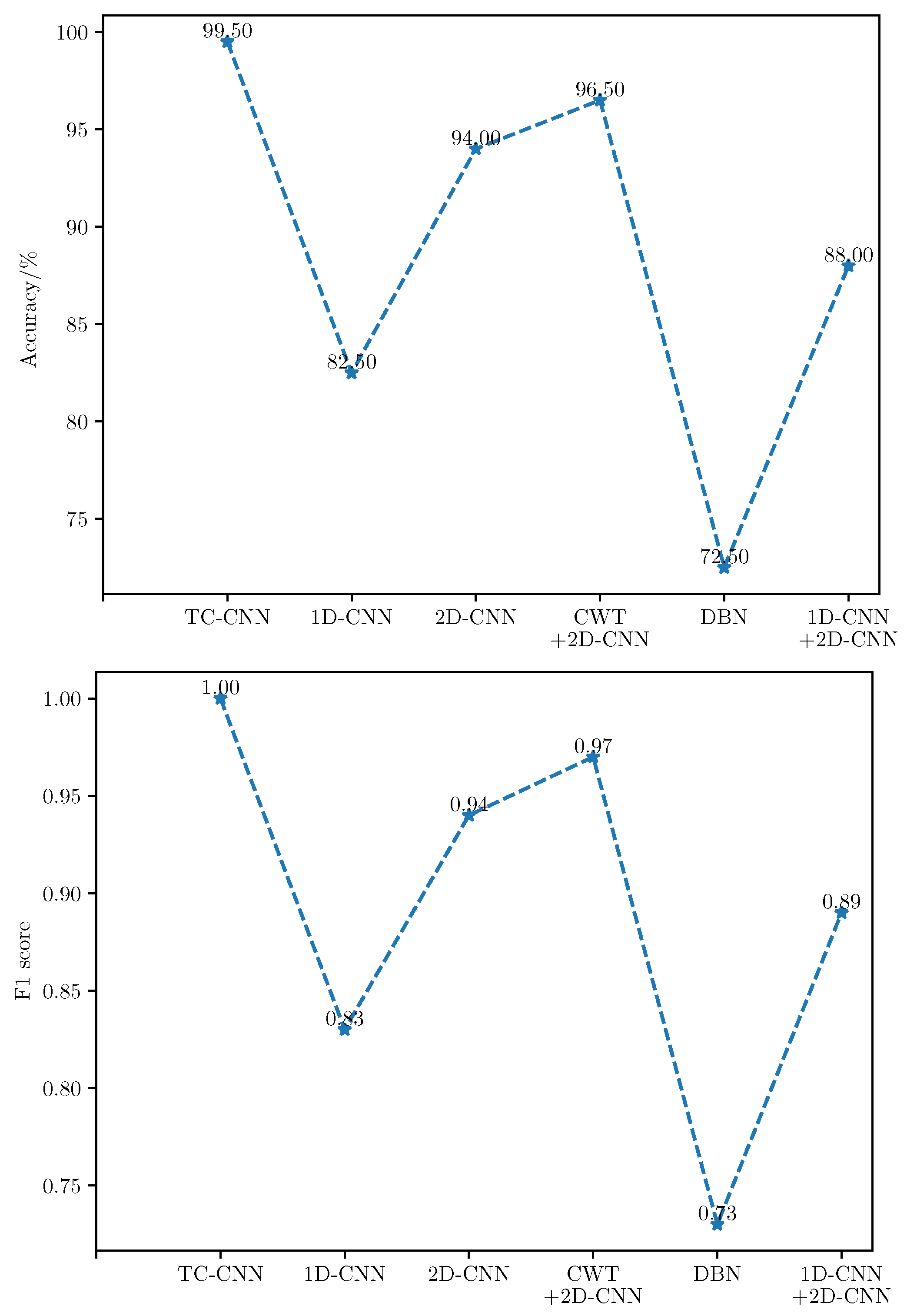
To avoid biased results due to random splits of the training and testing datasets, k-fold cross-validation is applied. All samples are divided into k mutually exclusive subsets of the same size, subsets are used as training samples, and the remaining subset is used as testing samples. The training samples are divided into the training set and validation set. A total of k experiments are performed to obtain k Accuracy and F1 score results, and the average is taken as the final experimental result. This paper set , the sample set is divided into 10 subsets, and the ratio of training set, validation set, and test set is set to: 7:2:1. The Accuracy and F1 score on balanced data samples are shown in Table 3 and Table 4 and Figure 10.
According to the results, it can be found that the methods with convolutional and pooling layers are more capable of fault diagnosis, and the DBN obtains the lowest values of Accuracy and F1 score among these models. Compared with the single-channel CNN model, the fault diagnosis performance of TC-CNN is improved due to information richness. Comparing 1D-CNN with 2D-CNN and CWT+2DCNN shows that 2D-CNN is generally better than 1D-CNN for fault diagnosis. 1D-CNN+2D-CNN also utilizes a two-channel model. Compared with single-channel CNN, its fault diagnosis effect is better than 1D-CNN but worse than 2D-CNN. The reason is that the inputs of both channels are original signals. When the data set is balanced, some extracted features are redundant or unimportant, leading to over-fitting of the model. The diagnostic results of the above-mentioned various models with balanced data sets verify the superiority of TC-CNN.
4.4. Fault Diagnosis Results under the Unbalanced Dataset
The diagnostic performance of TC-CNN is discussed in the previous section based on the balanced datasets. Traditional deep learning models need to be trained with a large number of samples to ensure good performance. In practice, however, the amount of faulty data is very small, and data imbalance is a common phenomenon. Therefore, it is necessary to solve the fault diagnosis problem under unbalanced datasets effectively. In this section, normal data and fault data are mixed in different proportions. The stability of TC-CNN for fault diagnosis is further demonstrated based on the experimental results of the datasets with different proportions. The normal and faulty samples in the training set are mixed in the ratios of 2:1, 5:1, 10:1, 20:1, 30:1, and 50:1, respectively. In the test set, the ratio of normal data to fault data is always 1:1. The distribution of the training set is shown in Table 5.
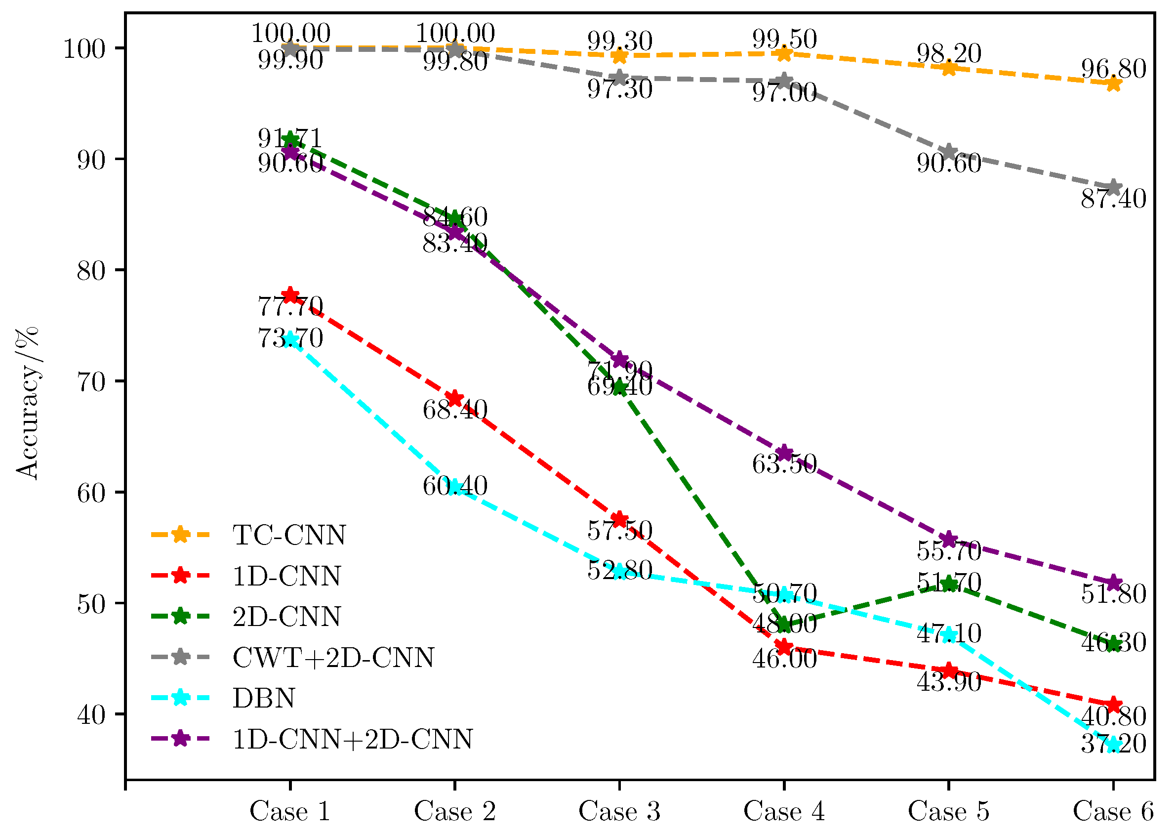
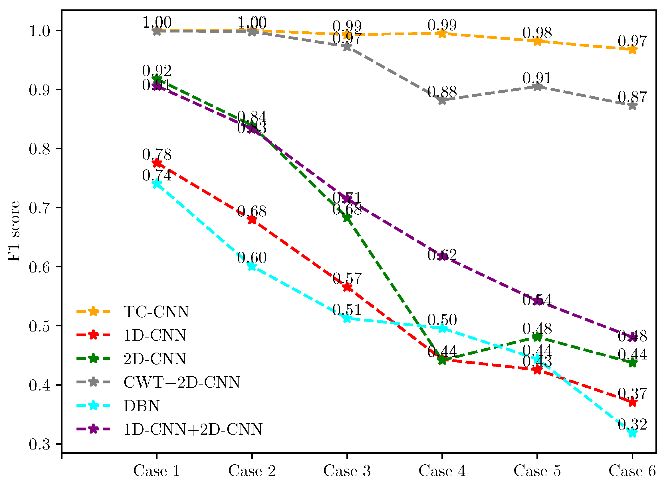
The fault diagnosis results are shown in Figure 11 and Figure 12. The fault detection capability of these methods varies with the number of fault samples. In case 1, the diagnostic Accuracy and F1 score for the six methods are (100.00%, 1.00), and (77.70%, 0.78), (91.71%, 0.92), (99.90%, 1.00), (73.70%, 0.74), and (90.60%, 0.91), respectively.
Then, in case 6, the number of faulty training samples is only 1/50 of the normal training samples, and the diagnostic Accuracy and F1 score of the proposed method are 96.80% and 0.97, respectively. The results of other methods are (40.80%, 0.37), (46.30%, 0.44), (46.30%, 0.44), (87.40%, 0.87), (37.20%, 0.32), and (51.80%, 0.48). When the ratio of the number of normal samples to the number of faulty samples reaches 50:1, TC-CNN still has excellent fault diagnosis ability. The diagnostic Accuracy is only 3.20% lower than in case 1, and the F1 score decreases by 0.03. On the contrary, the fault diagnosis performance of the remaining methods decreases significantly with the reduction of the fault sample size. When the fault data in the training dataset decrease as the imbalance rate increases, the model trained by these methods lacks a good ability to identify the fault data in this case. As a result, most of the faulty samples in the test dataset could not be classified correctly, resulting in low Accuracy and F1 score. When the imbalance ratio of data distribution increases, the superiority of the TC-CNN model gradually emerges. The TC-CNN model uses FFT and GST to add fault feature information, which extracts deeply into the data features and makes fault samples easier to distinguish.
When the imbalance ratio is small, such as 2:1, the diagnostic performance of TC-CNN is not much improved compared to CWT+2D-CNN. The feature richness advantage possessed by TC-CNN is relatively small when fault samples are balanced. When the data imbalance ratio is increased from 5:1 to 50:1, the fault diagnosis performance of TC-CNN does not decrease significantly compared with CWT+2D-CNN. Because CWT+2D-CNN only extracts time-frequency features, TC-CNN additionally extracts time-frequency features. The features of different dimensions complement each other, enrich the fault feature information, and make the fault samples easier to identify. When the imbalance ratios are 2:1 and 5:1, respectively, the fault diagnosis performance of 1D-CNN+2D-CNN is slightly lower than that of 2D-CNN. However, as the imbalance ratio gradually increases, the fault diagnosis performance of 1D-CNN+2D-CNN is better than that of 2D-CNN, indicating that 2D-CNN is more susceptible. The reason is that, when training samples are relatively sufficient, 1D-CNN+2D-CNN may extract some redundant features leading to overfitting of the model. However, when the data volume gradually decreases, 1D-CNN+2D-CNN can extract more features that can be utilized and, therefore, has better fault diagnosis performance. The fault diagnosis capability of TC-CNN is significantly stronger than that of 1D-CNN+2D-CNN because FFT and GST can extract more fault information with fewer fault samples, thus attenuating the effect of data imbalance. The training difficulty of DBN gradually increases as the number of training samples decreases, and it cannot effectively represent fault information. In addition, the DBN model has a limited ability to handle noise and other disturbing factors, thus significantly reducing its performance.
Therefore, TC-CNN has better fault diagnosis performance compared with traditional methods, although the severely unbalanced data set leads to performance degradation in all models. In the case of various data imbalance ratios, the TC-CNN model has excellent fault detection results and is less affected by the lack of fault data.
5. Conclusions
Summarizing the characteristics of the proposed method, firstly, the frequency domain features and time-frequency domain features are extracted using FFT and GST, respectively, which increases the dimensional of the extracted features, diversifies the fault features, and complements the fault information. Secondly, a two-channel model that combines 1D-CNN and 2D-CNN is proposed, with the frequency spectrum and time-frequency image as the input. Then, the features of individual channels are fused and incorporated into the training and learning process to achieve the fusion of feature layers. The experimental results show that the method can accurately identify different fault types and better fault diagnosis performance than many deep learning methods. In addition, the method shows good robustness and stability on highly unbalanced datasets. The limitation of the proposed method is that: the model input considered in this paper is a vibration signal. Using FFT and GST for feature extraction is very appropriate, which can achieve better fault diagnosis results. However, FFT and GST may not have good feature extraction effects for other types of features, such as current or sound signals. Using suitable feature extraction methods for current or sound signals is necessary. Therefore, the main work in the future is to research more effective feature extraction methods and further improve the fault diagnosis effect of the TC-CNN model under unbalanced datasets by fusing multiple types of signal features. Meanwhile, GAN can be combined with the proposed method in future work to achieve better diagnosis results.
Author Contributions
Conceptualization, Y.Q. and X.S.; methodology, Y.Q. and X.S.; validation, Y.Q. and X.S.; data curation, Y.Q.; writing—original draft preparation, Y.Q.; writing—review and editing, X.S. All authors have read and agreed to the published version of the manuscript.
Funding
This research received no external funding.
Institutional Review Board Statement
Not applicable.
Informed Consent Statement
Not applicable.
Data Availability Statement
This paper uses the rolling bearing fault diagnosis datasets of CWRU, which can be obtained from https://engineering.case.edu/bearingdatacenter/download-data-file. Last accessed on 21 August 2022. More detailed data used to support the results of this study are available from the corresponding authors upon request.
Conflicts of Interest
The authors declare no conflict of interest.
References
- Ma, B.; Cai, W.; Han, Y.; Yu, G. A novel probability confidence CNN model and its application in mechanical fault diagnosis. IEEE Trans. Instrum. Meas. 2021, 70, 3517111. [Google Scholar] [CrossRef]
- Yang, X.; Yan, X. A transferrable data-driven method for IGBT open-circuit fault diagnosis in three-phase inverters. IEEE Trans. Power Electron. 2021, 70, 13474–13488. [Google Scholar] [CrossRef]
- Samanta, A.; Chowdhuri, S.; Williamson, S.S. Machine learning-based data-driven fault detection/diagnosis of Lithium-Ion battery: A critical review. Electronics 2021, 10, 1309. [Google Scholar] [CrossRef]
- Zheng, Z.; Fu, J.; Lu, C.; Zhu, Y. Research on rolling bearing fault diagnosis of small dataset based on a new optimal transfer learning network. Measurement 2021, 177, 109285. [Google Scholar] [CrossRef]
- Rabah, A.; Abdelhafid, K. Rolling bearing fault diagnosis based on improved complete ensemble empirical mode of decomposition with adaptive noise combined with minimum entropy deconvolution. J. Vibroeng. 2018, 20, 240–257. [Google Scholar] [CrossRef]
- Andreas, K.; Robbersmyr, K.G. Cross-correlation of whitened vibration signals for low-speed bearing diagnostics. Mech. Syst. Signal Process. 2019, 118, 226–244. [Google Scholar] [CrossRef]
- Chen, Z.; Cen, J.; Xiong, J. Rolling bearing fault diagnosis using time-frequency analysis and deep transfer convolutional neural network. IEEE Access 2020, 8, 150248–150261. [Google Scholar] [CrossRef]
- Udmale, S.S.; Singh, S.K. Application of spectral kurtosis and improved extreme learning machine for bearing fault classification. IEEE Trans. Instrum. Meas. 2019, 68, 4222–4233. [Google Scholar] [CrossRef]
- Kannan, V.; Li, H.; Dao, D.V. Demodulation band optimization in envelope analysis for fault diagnosis of rolling element bearings using a real-coded genetic algorithm. IEEE Access 2019, 7, 168828–168838. [Google Scholar] [CrossRef]
- Roy, S.S.; Dey, S.; Chatterjee, S. Autocorrelation aided random forest classifier-based bearing fault detection framework. IEEE Sensors J. 2020, 20, 10792–10800. [Google Scholar] [CrossRef]
- He, J.; Yang, S.; Gan, C. Unsupervised fault diagnosis of a gear transmission chain using a deep belief network. Sensors 2017, 17, 1564. [Google Scholar] [CrossRef]
- Ma, M.; Sun, C.; Chen, X. Deep coupling autoencoder for fault diagnosis with multimodal sensory data. IEEE Trans. Ind. Informatics 2018, 14, 1137–1145. [Google Scholar] [CrossRef]
- Jing, L.; Zhao, M.; Li, P.; Xu, X. A convolutional neural network based feature learning and fault diagnosis method for the condition monitoring of gearbox. Measurement 2017, 111, 1–10. [Google Scholar] [CrossRef]
- Dixit, S.; Verma, N.K.; Ghosh, A.K. Intelligent fault diagnosis of rotary machines: Conditional auxiliary classifier GAN coupled with meta learning using limited data. IEEE Trans. Instrum. Meas. 2021, 70, 3517811. [Google Scholar] [CrossRef]
- Nasiri, A.; Taheri-Garavand, A.; Omid, M.; Carlomagnoc, G.M. Intelligent fault diagnosis of cooling radiator based on deep learning analysis of infrared thermal images. Appl. Therm. Eng. 2019, 163, 114410. [Google Scholar] [CrossRef]
- Gu, Y.; Cao, J.; Song, X.; Yao, J. A denoising autoencoder-based bearing fault diagnosis system for time-domain vibration signals. Wirel. Commun. Mob. Comput. 2021, 2021, 9790053. [Google Scholar] [CrossRef]
- Saucedo-Dorantes, J.J.; Arellano-Espitia, F.; Delgado-Prieto, M.; Osornio-Rios, R.A. Diagnosis methodology based on deep feature learning for fault identification in metallic, hybrid and ceramic bearings. Sensors 2021, 21, 5832. [Google Scholar] [CrossRef]
- Shao, H.; Jiang, H.; Zhao, H.; Wang, F. An enhancement deep feature fusion method for rotating machinery fault diagnosis. Knowl.-Based Syst. 2017, 119, 200–220. [Google Scholar] [CrossRef]
- Levent, E. Bearing fault detection by one-dimensional convolutional neural networks. Math. Probl. Eng. 2017, 2017, 8617315. [Google Scholar] [CrossRef]
- Pan, J.; Zi, Y.; Chen, J.; Zhou, Z.; Wang, B. LiftingNet: A novel deep learning network with layerwise feature learning from noisy mechanical data for fault classification. IEEE Trans. Ind. Electron. 2018, 65, 4973–4982. [Google Scholar] [CrossRef]
- Qiao, H.; Wang, T.; Wang, P.; Zhang, L.; Xu, M. An adaptive weighted multiscale convolutional neural network for rotating machinery fault diagnosis under variable operating conditions. IEEE Access 2019, 7, 118954–118964. [Google Scholar] [CrossRef]
- Peng, X.; Zhang, B.; Gao, D. Research on fault diagnosis method of rolling bearing based on 2DCNN. In Proceedings of the 2020 Chinese Control and Decision Conference, Hefei, China, 22–24 August 2020; pp. 693–697. [Google Scholar] [CrossRef]
- He, Z.; Shao, H.; Cheng, J.; Zhao, X.; Yang, Y. Support tensor machine with dynamic penalty factors and its application to the fault diagnosis of rotating machinery with unbalanced data. Mech. Syst. Signal Process. 2020, 141, 106441. [Google Scholar] [CrossRef]
- Chawla, N.V.; Bowyer, K.W.; Hall, L.O.; Kegelmeyer, W.P. SMOTE: Synthetic minority over-sampling technique. J. Artif. Intell. Res. 2002, 16, 321–357. [Google Scholar] [CrossRef]
- Tang, H.; Gao, S.; Wang, L.; Li, X.; Li, B.; Pang, S. A novel intelligent fault diagnosis method for rolling bearings based on wasserstein generative adversarial network and convolutional neural network under unbalanced dataset. Sensors 2021, 21, 6754. [Google Scholar] [CrossRef]
- Wang, Z.; Wang, J.; Wang, Y. An intelligent diagnosis scheme based on generative adversarial learning deep neural networks and its application to planetary gearbox fault pattern recognition. Neurocomputing 2018, 310, 213–222. [Google Scholar] [CrossRef]
- Mao, W.; Liu, Y.; Ding, L.; Li, Y. Imbalanced fault diagnosis of rolling bearing based on generative adversarial network: A comparative study. IEEE Access 2019, 7, 9515–9530. [Google Scholar] [CrossRef]
- Xuan, Q.; Chen, Z.; Liu, Y.; Huang, H.; Bao, G.; Zhang, D. Multiview generative adversarial network and its application in pearl classication. IEEE Trans. Ind. Electron. 2019, 66, 8244–8252. [Google Scholar] [CrossRef]
- Lee, Y.O.; Jo, J.; Hwang, J. Application of deep neural network and generative adversarial network to industrial maintenance: A case study of induction motor fault detection. In Proceedings of the IEEE International Conference on Big Data, Boston, MA, USA, 11–14 December 2017; pp. 3248–3253. [Google Scholar] [CrossRef]
- Han, T.; Liu, C.; Yang, W.; Jiang, D. A novel adversarial learning framework in deep convolutional neural network for intelligent diagnosis of mechanical faults. Knowledge Based Syst. 2019, 165, 474–487. [Google Scholar] [CrossRef]
- Akhenia, P.; Bhavsar, K.; Panchal, J.; Vakharia, V. Fault severity classification of ball bearing using SinGAN and deep convolutional neural network. Proc. Inst. Mech. Eng. Part J. Mech. Eng. Sci. 2022, 236, 3864–3877. [Google Scholar] [CrossRef]
- Tong, Q.; Lu, F.; Feng, Z.; Wan, Q.; An, G.; Cao, J.; Guo, T. A novel method for fault diagnosis of bearings with small and imbalanced data based on generative adversarial networks. Appl. Sci. 2022, 12, 7346. [Google Scholar] [CrossRef]
- Ruan, D.; Song, X.; Gühmann, C.; Yan, J. Collaborative optimization of CNN and GAN for bearing fault diagnosis under unbalanced datasets. Lubricants 2021, 9, 105. [Google Scholar] [CrossRef]
- Li, Y.; Xu, M.; Liang, X.; Huang, W. Application of bandwidth EMD and adaptive multiscale morphology analysis for incipient fault diagnosis of rolling bearings. IEEE Trans. Ind. Electron. 2017, 64, 6506–6517. [Google Scholar] [CrossRef]
- Liu, H.; Li, L.; Ma, J. Rolling bearing fault diagnosis based on STFT-deep learning and sound signals. Shock Vib. 2016, 2016, 6127479.1–6127479.12. [Google Scholar] [CrossRef]
- Cai, J.; Chen, Q. Bearing fault diagnosis method based on local mean decomposition and wigner higher moment spectrum. Exp. Tech. 2016, 40, 1437–1446. [Google Scholar] [CrossRef]
- Rauber, T.W.; de Assis Boldt, F.; Varejao, F.M. Heterogeneous feature models and feature selection applied to bearing fault diagnosis. IEEE Trans. Ind. Electron. 2015, 62, 637–646. [Google Scholar] [CrossRef]
- Gou, L.; Li, H.; Zheng, H.; Li, H.; Pei, X. Aeroengine control system sensor fault diagnosis based on CWT and CNN. Math. Probl. Eng. 2020, 2020, 5357146. [Google Scholar] [CrossRef]
- Xie, Y.; Zhang, T. Feature extraction based on DWT and CNN for rotating machinery fault diagnosis. In Proceedings of the 29th Chinese Control In addition, Decision Conference, IEEE, Chongqing, China, 28–30 May 2017; pp. 3861–3866. [Google Scholar] [CrossRef]
- Zhao, B.; Zhang, X.; Li, H.; Yang, Z. Intelligent fault diagnosis of rolling bearings based on normalized CNN considering data imbalance and variable working conditions. Knowl.-Based Syst. 2020, 199, 105971. [Google Scholar] [CrossRef]
- Saif, W.S.; Alshawi, T.; Esmail, M.A.; Ragheb, A.; Alshebeili, S. Separability of histogram based features for optical performance monitoring: An investigation using t-SNE technique. IEEE Photonics J. 2019, 11, 7203012. [Google Scholar] [CrossRef]
- Ma, L.; Yang, Y.; Wang, H. DBN based automatic modulation recognition for ultra-low SNR RFID signals. In Proceedings of the 2016 35th Chinese Control Conference, IEEE, Chengdu, China, 27–29 July 2016; pp. 7054–7057. [Google Scholar] [CrossRef]
Figure 1.
Frequency spectrum extraction using FFT.

Figure 2.
Generalized S-transform time-frequency image.

Figure 3.
A typical CNN structure.

Figure 4.
Flowchart of the proposed TC-CNN structure used for rolling bearing fault diagnosis.

Figure 5.
Rolling bearing experimental facility.

Figure 6.
Feature visualization of input data.

Figure 7.
Feature visualization of fully connected layer .

Figure 8.
Feature visualization of fully connected layer .

Figure 9.
Feature visualization of fully connected layer .

Figure 10.
Comparison of test set fault diagnosis results.

Figure 11.
Accuracy of different methods for six unbalanced dataset cases.

Figure 12.
F1 scores of different methods for six unbalanced dataset cases.


Table 1.
Rolling bearing fault information.
| Location | Fault Diameter (inch) | Fault Orientation | Label |
|---|---|---|---|
| Ball | 0.007 | - | |
| Ball | 0.014 | - | |
| Ball | 0.021 | - | |
| Inner race | 0.007 | - | |
| Inner race | 0.014 | - | |
| Inner race | 0.021 | - | |
| Outer race | 0.007 | Center @6:00 | |
| Outer race | 0.014 | Center @6:00 | |
| Outer race | 0.021 | Center @6:00 | |
| Normal | - | - |
Table 2.
Parameters of the TC-CNN.
| Layer Name | Parameter | Layer Size |
|---|---|---|
| - | ||
| - | ||
| Conv(), kernel size = 6 | ||
| Conv(), kernel size = 5 | ||
| kernel size = 4 | ||
| kernel size = 2 | ||
| Conv(), kernel size = 5 | ||
| Conv(), kernel size = 5 | ||
| kernel size = 3 | ||
| kernel size = 2 | ||
| - | 656 | |
| - | 2704 | |
| - | 3360 | |
| D | - | 3360 |
| 84 | ||
| SVM | 10 | |
| O | - |
Table 3.
The comparison of fault diagnosis accuracy.
| Method | Accuracy (%) | ||
|---|---|---|---|
| Training Set | Validation Set | Test Set | |
| TC-CNN | 100.00 | 99.50 | 99.50 |
| 1D-CNN | 100.00 | 81.25 | 82.50 |
| 2D-CNN | 100.00 | 95.00 | 94.00 |
| CWT+2DCNN | 97.71 | 96.25 | 96.50 |
| DBN | 100.00 | 74.00 | 72.50 |
| 1D-CNN+2D-CNN | 100.00 | 91.00 | 88.00 |
Table 4.
The comparison of F1 score.
| Label | Method | |||||
|---|---|---|---|---|---|---|
| TC-CNN | 1D-CNN | 2D-CNN | CWT+2DCNN | DBN | 1D-CNN+2D-CNN | |
| 1.00 | 0.74 | 0.86 | 0.94 | 0.58 | 0.73 | |
| 1.00 | 0.70 | 0.77 | 0.96 | 0.71 | 0.75 | |
| 1.00 | 0.87 | 1.00 | 0.90 | 1.00 | 1.00 | |
| 1.00 | 0.81 | 1.00 | 1.00 | 0.58 | 0.87 | |
| 0.98 | 0.71 | 0.92 | 0.98 | 0.51 | 0.88 | |
| 1.00 | 0.81 | 1.00 | 1.00 | 0.72 | 0.89 | |
| 1.00 | 0.96 | 1.00 | 1.00 | 0.74 | 0.97 | |
| 1.00 | 1.00 | 1.00 | 0.90 | 1.00 | 1.00 | |
| 1.00 | 0.81 | 0.95 | 1.00 | 0.52 | 0.83 | |
| 1.00 | 0.98 | 0.97 | 1.00 | 0.96 | 1.00 | |
| F1 score (macro) | 1.00 | 0.83 | 0.94 | 0.97 | 0.73 | 0.89 |
Table 5.
Distribution of the training dataset.
| Unbalanced Cases | Size of Normal Condition | Size of Each Kind of Fault Conditions | |||
|---|---|---|---|---|---|
| Training Dataset | Testing Dataset | Training Dataset | Testing Dataset | ||
| Case 1 | 2:1 | 300 | 100 | 150 | 100 |
| Case 2 | 5:1 | 300 | 100 | 60 | 100 |
| Case 3 | 10:1 | 300 | 100 | 30 | 100 |
| Case 4 | 20:1 | 300 | 100 | 15 | 100 |
| Case 5 | 30:1 | 300 | 100 | 10 | 100 |
| Case 6 | 50:1 | 300 | 100 | 6 | 100 |
Publisher’s Note: MDPI stays neutral with regard to jurisdictional claims in published maps and institutional affiliations. |
© 2022 by the authors. Licensee MDPI, Basel, Switzerland. This article is an open access article distributed under the terms and conditions of the Creative Commons Attribution (CC BY) license (https://creativecommons.org/licenses/by/4.0/).
Share and Cite
MDPI and ACS Style
Qin, Y.; Shi, X. Fault Diagnosis Method for Rolling Bearings Based on Two-Channel CNN under Unbalanced Datasets. Appl. Sci. 2022, 12, 8474. https://0-doi-org.brum.beds.ac.uk/10.3390/app12178474
AMA Style
Qin Y, Shi X. Fault Diagnosis Method for Rolling Bearings Based on Two-Channel CNN under Unbalanced Datasets. Applied Sciences. 2022; 12(17):8474. https://0-doi-org.brum.beds.ac.uk/10.3390/app12178474
Chicago/Turabian StyleQin, Yufeng, and Xianjun Shi. 2022. "Fault Diagnosis Method for Rolling Bearings Based on Two-Channel CNN under Unbalanced Datasets" Applied Sciences 12, no. 17: 8474. https://0-doi-org.brum.beds.ac.uk/10.3390/app12178474
Note that from the first issue of 2016, this journal uses article numbers instead of page numbers. See further details here.