Evaluation of Multiple Linear Regression and Machine Learning Approaches to Predict Soil Compaction and Shear Stress Based on Electrical Parameters

Abstract

This study investigated the relationships between the electrical and selected mechanical properties of soil. The analyses focused on comparing various modeling relationships under study methods that included machine learning methods. The input parameters of the models were apparent soil electrical conductivity and magnetic susceptibility measured at depths of 0.5 m and 1 m. Based on the models, shear stress and soil compaction were predicted. Neural network models outperformed support vector machines and multiple linear regression techniques. Exceptional models were developed using a multilayer perceptron neural network for shear stress (R = 0.680) and a function neural network for soil compaction measured at a depth of 0–0.5 m and 0.4–0.5 m (R = 0.812 and R = 0.846, respectively). Models of very low accuracy (R < 0.5) were produced by the multiple linear regression.

1. Introduction

Smart agriculture dates back to the 1980s when the Global Positioning System became available to the general public. Precision agriculture helps farmers to improve productivity and quality by using minimal resources such as water, fertilizer, pesticides, and seeds [1]. Soil contains a mixture of different shapes, mineralogy, and particle sizes, which has a significant effect on soil behavior. Soils can be classified based on grain size and grain size distribution [2]. Conductivity measures the potential of a material to convey an electrical charge. Lund [3] and Barbosa et al. [4] described soil electrical conductivity (ECa) as the measurement corresponding to soil properties affecting crop productivity and soil texture, drainage conditions, and organic matter content. Soil conductivity relates strongly to soil grain size and texture [4]. Because clay soils hold more moisture and have a greater surface area, ensuring more particle-to-particle contact, it is a better conductor than sand or silts [5]. Soil conductivity can be measured in the field using the physical, direct contact of four electrodes with soil or via electromagnetic induction (EMI), which uses a transmitter coil to induce a field into the soil and a receiver coil to measure the response [3]. Othaman et al. [6] revealed that soil electrical conductivity is directly proportional to the nutrient concentration in soil and inversely proportional to soil depth. Moreso, soil electrical conductivity reflects soil salinity, i.e., the higher the ECa value, the higher the soil salinity, and vice versa.

Magnetic susceptibility (MS) refers to the physical quantity describing material properties in the external magnetic field [7,8]. The measurement of magnetic susceptibility is important in identifying the properties, factors, and processes of soil formation, and it applies to soil mapping [9]. Magnetic susceptibility can be measured with the use of a susceptometer. It is used when magnetic measurements may not be possible and has a broad dynamic resonant frequency range based on a proximity detector oscillator [10].

Some scanning methods and tools are used, in practice, to assess soil parameters based on the measurement of soil electrical conductivity and magnetic susceptibility. ARP03 (automated resistivity profiling) is a multi-pole scanning method that uses a computer-assisted acquisition tool to produce high-resolution maps of electrical resistivity. It generates data in real-time through a distinctive global positioning system [11]. This mobile system is an effective method of characterizing agricultural subsoil and allows for the execution of continuous resistivity profiling without a fixed device. Geophilus electricus (Geophilus) is another scanning system used to map complex electrical resistivity in soils [12]. Combined with GPS, it measures complex values of electrical resistivity in terms of amplitude (electrical conductivity) and phase (soil compaction) of up to 1.5 m in depth. This system is also used to image soil layers and their geometry with depth. Another system is the Veris 3100, which is an electrode-based system that makes direct contact with soil and records measurements by pulling sensors across the field. It records two ECa measurements simultaneously using six rolling electrodes at two different depths every second [13].

Scanning methods are widely used in the determination of agricultural management zones (MZ). Sentinel-2 satellite is a valid scanning method for delineating the management zone in the milieu of precision agriculture, as additional data is not required. Rokhafrouz et al. [14] stated that MZ delineation can be ameliorated by integrating soil, crop, and yield information and knowledge of agronomy and climate. Satellite-derived NDVI (normalized difference vegetation index) is useful for delineating management zones. Mazur et al. [15] stated that the stability of soil chemical properties (pH, P, K, and Mg) that can be used for stratified soil sampling is due to management zone delineation. The online visible and near-infrared (vis–NIR) spectroscopy sensors are methodical in depicting water-holding capacity zones for site-specific irrigation [16]. It also has a strong relationship with moisture content, clay content, and the plasticity index.

The increase in agricultural mechanization and the need to maximize agricultural yields globally have influenced soil compaction [17]. Soil compaction is a substantial form of soil degradation [18] caused by compression from machinery traffic, stock trampling, and humans [19,20], and these also affect trees and shrubs [21]. Soil compaction takes place when soil mislays its natural resistance to the movement of machinery [22] and presents a major problem, resulting in inadequate rooting systems, poor yields [23], low soil fertility, and increased soil erosion [24]. Soil compaction reduces soil porosity, increases soil density and penetration resistance, decreases infiltration, degrades the soil structure, and limits root growth [25,26,27]. Soil compaction is a resultant side effect of land-use intensification. Moreover, increased compaction increases nitrous oxide (N₂O) emissions [28].

Shear stress refers to the force that causes the deformation of materials by slippage along a plane parallel to the imposed stress, which may occur in solids or liquids, and the resultant shear is related to the downslope movement of the earth materials. Soil shear stress depends on soil characteristics, granular composition, humus content, humidity, root density, and the degree of vegetation cover in the case of vegetated areas. Researchers have proven that shear stress induces an ambiguous pore system with vertical and horizontal soil displacement, decreases permeability, and causes excess surface runoff during strong rainfall [29]. Shear stress affects soil structure by drastically reducing macro-porosity and saturated hydraulic conductivity in topsoil [30]. An increase in wheel slip and traction force results in shear stress rising, which may steer the detachment of a weak topsoil layer exposed to erosion and surface runoff [31].

An effective perspective for managing agricultural land variability is the implementation of MZ. An agricultural management zone depicts an area or region of an agricultural field that is inconsistent with the rest of the field and can be managed with a specific, single-rate management practice to maximize yields and environmental impacts [14,32]. The agricultural management zone aims to ensure that no information vital for crop management is lost [33]. Under fast-changing climatic conditions, the management zone is prone to uncertainty, especially in situations where knowledge of agronomy and climate are not incorporated [14].

Artificial intelligence (AI) and machine learning (ML) methods are extensively used to model complex relationships in agriculture [34,35,36,37,38], including soil properties. Yang et al. [39] compared four ML methods, namely, partial least squares regression, least squares support vector machines (SVM), extreme learning machines, and the Cubist regression model employed for the prognosis of soil organic matter and pH. Five machine learning models, including multilayer perceptron and support vector regression, were developed by Wang et al. [40] for the estimation of soil salinity. Bouslihim et al. [41] found random forest and multiple linear regression (MLR) methods to be accurate tools for approximating soil aggregate stability. Wu et al. [42] compared ten machine learning techniques and reported the generalized regression neural network model as an effective method for the evaluation of soil nutrient content. Chen et al. [43] used different machine learning algorithms and stated that random forests, improved by the polarimetric decomposition of parameters, outperformed support vector regression and gradient boosting regression trees. Another promising machine learning approach is Gaussian process regression (GPR). This technique avoids some limitations of data-driven approaches (e.g., neural networks, support vector machines) and produces better models of performance [44,45].

Precision and digital agriculture both rely on the acquisition, processing, and exploitation of large amounts of data, including the soil environment of plant growth and the operation of agricultural machinery. Dynamic field probes measuring the mechanical parameters of agricultural soils play a special role here. Some of them allow for the measurement of soil compactness—understood as cone penetrometric resistance in the vertical profile and in the horizontal plane—over several layers [46]. Others, such as the probe developed by the team of Aguera et al. [47] make it possible to measure soil shear resistance at different depths of the soil profile of a plowing. Unfortunately, these concepts are not yet commercially available. The research into new solutions for monitoring and predicting soil shear stress, compactness, and penetrometric resistance seems justified. Soil shear stress, compaction, electrical conductivity, and magnetic susceptibility correlate significantly with related soil parameters such as soil texture (clay content), bulk density, moisture content, and organic matter content. Therefore, it is reasonable to use ECa and MS scanning as an indirect method to estimate soil shear stress and soil compactness. On the other hand, the prediction of soil shear stress from indirect measurements and other physico-mechanical parameters of soils in agriculture and agrophysics is not a new approach. Zhu et al. [48] invented a method to predict soil shear strength parameters (cohesion and internal friction angle) by combining cone penetration test (CPT) data and soil properties such as bulk density and water content. Using methods of machine learning for prediction, they obtained a prediction error of R = 0.87. Vanapalli et al. [49] attempted to predict shear strength on the basis of soil suction. Thirdly, soil electrical conductivity and magnetic susceptibility measurement platforms and probes are currently the most widely used and adopted in agricultural advisory practices. Research into their alternative uses is, therefore, the subject of this study.

This research aimed to compare the performance of multiple linear regression, two types of artificial neural networks (ANN), and support vector machines to predict soil compaction and the shear stress of clay soil based on apparent conductivity and magnetic susceptibility. As a result of the prediction of these parameters, soil traction performance can be estimated. In addition, energy loss resulting from the transfer of tractor driving force on the soil can be minimized. It can be used in practice, e.g., in controlled traffic farming.

2. Materials and Methods

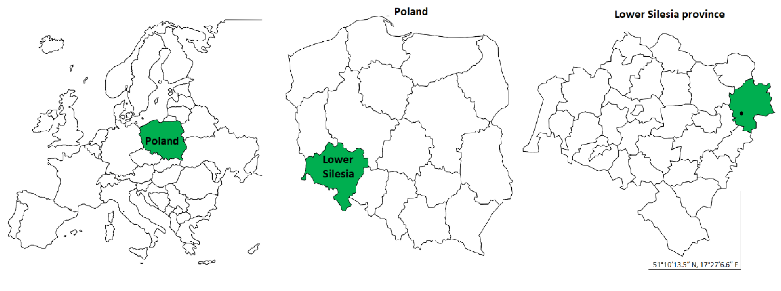
2.1. Experimental Data Acquisition

In the summer of 2019, soil sampling was conducted in the Oleśnica district, Lower Silesia province of Poland, on a 12.86 ha field (Figure 1). After the combined harvesting of winter oilseed rape grown in the 2018–2019 growing season, a universal cultivator, Horsh Terrano, was used to cultivate the field at a depth of 0.01 m. This was preceded by measurement procedures in accordance with the Polish Soil Classification System [50] and USDA Soil Taxonomy [51], which classified the soil as sandy clay loam (sand 57.3%, clay 24.3%, and silt 18.4%).

The Geonics EM38 conductivity meter [52] is a movable field instrument designed to approximate soil ECa and MS in the rooting zone (depth of 1.5 m). Its high speed and accuracy support broadscale soil conductivity measurements. EM38 sets up a primary electromagnetic field; small horizontal electrical currents in the soil are induced, and as a result, a subsequent electromagnetic field is generated. It has a built-in receiver coil that detects both fields, and the proportion of these is the measurement of ECa displayed in units of ms·m⁻¹. EM38 measures electrical conductivity either vertically (EM38V), with a theoretical depth response curve of 0 to 1.5 m, or horizontally (EM38H), with a theoretical depth response curve of 0 to 1 m [53], and allows for a faster method of determining if conductivities increase or decrease with depth. Soil moisture equaled 30% measured over a short interval after the EM38 survey; temperature was equal to 15 °C.

Using the cone penetrometer (Eijkelkamp Soil & Water, Giesbeek, The Netherlands) with GPS, soil compaction was measured for a soil layer between 0–0.5m. A cone with a base of 0.0001 m² and an angle of 60° was used during field measurements with a penetration speed of 0.03 m·s⁻¹. After measuring electrical parameters and analyzing the results, a total of five management zones were mapped. In a 30 m grid, soil compaction measurements were conducted, and coordinates were assigned to each measured point based on the GPS position of the Eijkelkamp Penetrologger. The nearest point of soil electrical conductivity and magnetic susceptibility measurements were linked to each spot of soil compaction measurement using the least-squares method. Based on previous research [54], soil compaction was estimated at a depth of 0–0.5 m, and between 0.4 and 0.5 m was chosen for further analysis.

For shear stress measurement, the field inspection tester VANE-H60 (Eijkelkamp Soil & Water, The Netherlands) was used. This tool allows for a swift determination of soil shear stress. It comprises exchangeable vanes of different dimensions (16 × 32, 20 × 40, 25.4 × 50.8 mm (extended)) and many 0.5-m rods. This equipment makes it possible, depending on the vane used, to measure shear stress between 0 and 260 kPa. The peak value is determined using a scale ring, which must be turned back to the zero position before and after every measurement. The extension rods are specially designed to provide the connection maximum with bending resistance. It has a maximum measuring depth of 3 m (reasonable correlation to full-scale field vane tests), shear stress of 260 kPa, measuring accuracy of <±10%, and reading accuracy of 1%. Dummy tests were performed with rods only to perfect the skin friction of the extension rods. The measurement of shear stress was conducted at the depth of 0.25 m. The measurement points (GPS positions) for shear stress and the method for linking ECa and MS measurements were the same as in the case of soil compaction.

2.2. Multiple Linear Regression

MLR is the most commonly used linear regression model. It is a multivariate statistical technique used to elucidate the relationship between multiple independent variables (X₁, X₂,…, X_k) and a dependent variable (Y) with an explanation and prediction as objectives:

• The explanation objective examines the regression coefficients and their magnitude, sign, and statistical inference for each predictor variable;
• The forecast objective examines the extent to which the explanatory variables can estimate the explicative variable [55].

MLR prediction models are shown as follows:

Y_t = X_tβ + ε_t

(1)

where Y_t is the estimated value at time t, β = (β₀, β₁, …, β_k) is an indication of the relationship between the independent and dependent variables, and X_t = (1, x_1t, x_2t, …, x_jt) is a vector of j-dependent variables at time t. ε_t is a random error term at time t, t = 1, …, N. The error terms should be independent and show a Gaussian distribution behavior. The presumptions of the MLR model could be examined by the Kolmogorov–Smirnov test and the Q* Ljung–Box statistic, as in the timeseries.

2.3. Artificial Neural Networks

ANN is a computer learning system inspired by the functioning of the human nervous system. ANNs are made up of artificial neurons (simple information-processing units) displayed in layers. A minimum of two layers of artificial neurons are necessary for the artificial neural network system—input and output layers. The two types of neural networks used for modeling the relationships under study are the multilayer perceptron (MLP) and radial basis function (RBF) neural networks. In an MLP network, the signal is processed from the input layer through one or two hidden layers to the output layer. Connection weights in MLP are adjusted during the training process by a backpropagation algorithm. An RBF network is a feedforward neural network with only one hidden layer. The activation function of neurons in a hidden layer is usually a Gaussian function [56]. The linear neuron is responsible for the calculation of the RBF network’s output signal. Radial basis function neural networks have generally better forecasting abilities and faster learning speeds in comparison with other neural networks [57].

A set of 154 data was acquired from measurements. The dataset was randomly distributed between training and validation sets in the ratio of 80:20. The data were normalized in a range of <0; 1> before the training process of the neural models. In this study, both the multilayer perceptron and the radial basis function neural models were developed in the Statistica v. 13 software. The input vector comprised a combination of apparent soil electrical conductivity and magnetic susceptibility measured at depths of 0.5 m and 1 m. As an output model parameter, the compaction of certain soil layers or shear stress was used. The form of the input vector determined the number of nodes in the input layer (four). For each model, 2000 different neural structures were trained. Each neural model was characterized by the type of neural network (MLP or RBF), the number of neurons in the hidden layer, and the initial connection weight matrix. The number of neurons in the hidden layer was changed in a range of 10–40. In the case of the multilayer perceptron network, various transfer functions for the neurons in the hidden and output layers were used (sigmoidal, hyperbolic tangent, and exponential).

2.4. Sensitivity Analysis

Sensitivity analysis is a method to emphasize the contribution of independent input variables in the ANN model. We used Statistica v. 13 environments for the sensitivity analysis to provide information about the relative importance of the inputs. Here, the average values replaced the values of each input variable determined using the training dataset. A proportion of two errors is calculated in this method: the error with a certain input replaced by its mean and the error with the original input values. The error ratio can be interpreted as the importance of the input parameter and is used to estimate the degree of influence expressed in percentages the input parameters of an ANN model have on its output. Hadzima-Nyarko et al. [58] used a similar sensitivity analysis in the prediction and analysis of structural damage after an earthquake.

2.5. Support Vector Machines

SVM is a technique widely implemented for the categorization of nonlinear regression. It was first proposed by Vapnik [59]. There is a wide availability of published materials describing the theoretical background of SVM [60,61]. The ε-SVM regression model was implemented for this research. The training dataset is required to apply the SVM technique. The structure of the dataset is as follows: (x₁,y₁), (x₂,y₂), (x₃, y₃), …, (x_n, y_n) where x∈𝕽^m is the input data and y_i∈𝕽 is the corresponding target. The objective of a support vector machine is to estimate the regression function, defined as:

$$f\left(x\right)=w^T\phi \left(x\right)+b$$

(2)

where w∈𝕽^m is the vector of weights and b is the bias.

During the training process, vector w is optimized as long as the deviation from the actual target is less than the predetermined constant, ε, which can be described as:

$$Min \frac{1}{2}{⃦w⃦}^2$$

(3)

subject to

$$y_i-w^T{x}_i-b\le \epsilon$$

(4)

$$w^T{x}_i+b-y_i\le \epsilon$$

$$i=1, \dots , n.$$

Vapnik [62] introduced the nonnegative slack variables $\xi$ and ${\xi }^{*}$ to deal with the feasible constraints of the above optimization problem. This changed the problem in (2) to the following form (for nonlinear regression):

$$Min \frac{1}{2}{⃦w⃦}^2+C{{\displaystyle \sum }}_{i=1}^n{\xi }_i+C{{\displaystyle \sum }}_{i=1}^n{\xi }_i^{*}$$

(5)

subject to the constraints

$$y_i-w^T\phi \left(x_i\right)-b\le \epsilon +{\xi }_i$$

(6)

$$w^T\phi \left(x_i\right)+b-y_i\le \epsilon +{\xi }_i^{*}$$

$${\xi }_i, {\xi }_i^{*}\ge 0, i=1, \dots , N$$

where C is the capacity constant, which can be interpreted as a coefficient of a penalty, and φ(x) is the kernel function, which is decisive for the SVM model performance. In this research, the Gaussian radial basis function (7) was employed.

$$K\left(x_i,x\right)=\exp (-\gamma |\left|x-x_i\right|{|}^2)$$

(7)

In the case of an ε-SVM regression model with RBF kernel function, the three parameters, namely, γ, should be modified to optimize the generalization capacity of the model. In this study, the optimum values of the C, ε, and γ parameters were found with a trial-and-error method. In total, 75% of the data was randomly chosen as a training set and 25% of the data was used as a validation set. The ten-fold cross-validation method was used. The Statistica v. 13 software was used for the development of support vector machine models.

2.6. Criteria of Accuracy Assessment of Models

Five parameters were used in this research for the evaluation of the accuracy of regression models: coefficient of correlation (R), root mean squared error (RMSE), mean absolute error (MAE), mean absolute percentage error (MAPE), and Nash–Sutcliffe coefficient (NSC). These metrics were calculated according to the following equations:

$$R=\frac{{{\displaystyle \sum }}^{\text{}}(Y_{meas}-{\overline{Y}}_{meas})\left(Y_{pred}-{\overline{Y}}_{pred}\right)}{\sqrt{{{\displaystyle \sum }}^{\text{}}{(Y_{meas}-{\overline{Y}}_{meas})}^2{{\displaystyle \sum }}^{\text{}}{\left(Y_{pred}-{\overline{Y}}_{pred}\right)}^2}}$$

(8)

$$RMSE=\sqrt{\frac{1}{n}{{\displaystyle \sum }}_{i=1}^n{\left(Y_{pred}-Y_{meas}\right)}^2}$$

(9)

$$MAE=\frac{1}{n}{{\displaystyle \sum }}_{i=1}^n\left|Y_{pred}-Y_{meas}\right|$$

(10)

$$MAPE=\frac{1}{n}{{\displaystyle \sum }}_{i=1}^n\left|\frac{Y_{meas}-Y_{pred}}{Y_{meas}}\right|$$

(11)

$$NSC=1-\left[\frac{{{\displaystyle \sum }}_{i=1}^n{\left(Y_{meas}-Y_{pred}\right)}^2}{{{\displaystyle \sum }}_{i=1}^n{\left(Y_{meas}-{\overline{Y}}_{pred}\right)}^2}\right]$$

(12)

where Y_pred is the absolute predicted value, ${\overline{Y}}_{pred}$ is the mean predicted value, Y_meas is the absolute measured value, ${\overline{Y}}_{meas}$ is the mean measured value, and n is the amount of data in a dataset.

The high values of R and NSC and low values of RMSE, MAE, and MAPE are not reliable enough for ML model assessment. Therefore, the multi-criteria approach [63,64] was used, and the generalization ability (GA) was the additional metric calculated for the ANN and SVM models. GA, defined by Yoon et al. [65], is calculated as follows:

$$GA=\frac{RMS{E}_{validation}}{RMS{E}_{train}}$$

(13)

El Bilali et al. [66] suggested the following classification of prediction models based on GA metrics:

• The model is perfect if GA  =  1;
• The model is excellent if 0.75 ≤ GA < 1 or 1 < GA ≤ 1.35;
• The model is good if 1.35 < GA ≤ 2 or 0.5 ≤ GA < 0.75;
• The model is poor and unsuitable for prediction if GA > 2 or GA < 0.5.

The objective function (OBJ) used for the multi-criteria assessment of the precision of machine learning models was calculated according to the following equation:

$$OBJ=\left(\frac{N_T-N_V}{N_T+N_V}\right)\frac{RMS{E}_T+MA{E}_T}{R_T^2+1}+\left(\frac{2N_V}{N_T+N_V}\right)\frac{RMS{E}_V+MA{E}_V}{R_V^2+1}$$

where N_T is the amount of data in the training dataset and N_V is the amount of data in the validation (testing) dataset. The lower value of OBJ indicates a more accurate model.

3. Results

The statistics of the experimental data (physical soil properties) are detailed in

Table 1. Statistics of the experimental data.

The Parameter	Minimum	Maximum	Mean	Standard Deviation
Soil compaction (depth 0–0.5 m) (MPa)	0.65	2.20	1.41	0.28
Soil compaction (depth 0.4–0.5 m) (MPa)	0.17	3.39	1.14	0.58
Shear stress (kPa)	96.00	248.00	163.40	32.88

.

As shown in Table 1, the mean value of the soil compaction was lower when measured for a thinner soil layer of 0.1 m between 0.4 and 0.5 m in depth.

3.1. Multiple Linear Regression

Three MLR models were developed in this study. The first regression model used soil compaction (depth 0.4–0.5 m) as the output parameter (RSC_0.4_0.5). The second one used soil compaction (depth 0–0.5 m) as the output parameter (RSC_0_0.5). The third regression model (RSS) used shear stress as the output. All regression models were based on four independent variables (apparent soil electrical conductivity measured at a depth of 0.5 m, apparent soil electrical conductivity measured at a depth of 1 m, magnetic susceptibility measured at a depth of 0.5 m, and magnetic susceptibility measured at a depth of 1 m). Detailed results of the MLR analysis variables are presented in

Table 2. Regression coefficients and probability levels for regression models.

Factor	RSC_0.4_0.5 Constant Term = 1.812				RSC_0_0.5 Constant Term = 1.545				RSS Constant Term = 124.587
	b Coefficient	Standard Error b	p-Value	Significance	b Coefficient	Standard Error b	p-Value	Significance	b Coefficient	Standard Error b	p-Value	Significance
Apparent soil electrical conductivity 0.5 m (ECa0.5)	0.390	0.094	0.017	+	−0.040	0.008	<0.001	+	5.530	1.065	<0.001	+
Magnetic susceptibility 0.5 m (MS0.5)	−0.837	0.089	0.749	−	−1.868	1.238	0.133	−	146.434	147.712	0.323	-
Apparent soil electrical conductivity 1 m (ECa1)	0.390	0.132	0.038	+	0.009	0.005	0.083	−	−1.192	0.644	0.066	-
Magnetic susceptibility 1 m (MS1)	−0.077	0.139	0.502	−	−0.025	0.054	0.642	−	−18.247	6.549	0.006	+

Determination of the level of statistical significance: − nonsignificant; + significant for α = 0.05.

.

The constant term (sometimes called the “intercept”) in a regression model represents the mean value of the response variable when all of the predictor variables in the model are equal to zero.

The beta coefficient (b coefficient) is the degree of change in the outcome variable for every one unit of change in the predictor variable.

The p-values for the coefficients indicate whether these relationships are statistically significant. A low p-value (<0.05) means that the coefficient is likely not to equal zero. A high p-value (>0.05) means that we cannot conclude that the explanatory variable affects the dependent variable. A high p-value is also called an insignificant p-value.

MS measured at 0.5 m of depth is a variable for which statistical significance was not confirmed at the α = 0.05 level in any of the developed models, while magnetic susceptibility measured at a depth of 1 m was a statistically significant trait only in the RSS model. In the RSC_0.4_0.5 model, the statistically significant traits were ECa0.5 and ECa1. In the RSC_0_0.5 model, the only statistically significant trait was ECa0.5. The statistically significant traits in the RSS model were ECa0.5 and MS1.

Based on the outcome from Table 2, and examining only statistically significant traits, multiple regression equations describing each model are as follows:

RSC_0.4_0.5 = 1.812 − (0.045 × ECa0.5) + 0.023 × ECa1

(14)

RSC_0_0.5 = 1.545 − (0.040 × ECa0.5)

(15)

RSS = 124.587 + 5.530 × ECa0.5 − (18.247 × MS1)

(16)

Error metrics for multiple linear regression models are detailed in

Table 3. Error metrics of multiple linear regression models.

Model	RMSE	MAE	MAPE	NSC	R
RSC_0.4_0.5	0.535	0.401	28.468	0.152	0.408
RSC_0_0.5	0.335	0.261	18.187	0.072	0.469
RSS	37.794	30.433	21.299	0.073	0.423

.

3.2. Artificial Neural Networks

For each soil physical parameter, namely, soil compaction (depth 0.4–0.5 m), soil compaction (depth 0–0.5 m), and shear stress, two neural models were developed with the use of MLP (MLPSC_0.4_0.5, MLPSC_0_0.5, and MLP_SS) and RBF (RBFSC_0.4_0.5, RBFSC_0_0.5, and RBF_SS) neural network. The structures of the models and error metrics are presented in

Table 4. Structures and error metrics of the best MLP neural models.

Model	Model Structure	Train					Validation					GA	OBJ
		RMSE	MAE	MAPE	NSC	R	RMSE	MAE	MAPE	NSC	R
MLPSC_0_0.5	4-12-1	0.246	0.191	15.416	0.297	0.545	0.153	0.134	9.550	0.555	0.790	0.621	0.281
MLPSC_0.4_0.5	4-10-1	0.471	0.355	21.302	0.319	0.567	0.387	0.323	20.246	0.546	0.772	0.821	0.562
MLP_SS	4-19-1	29.363	23.289	14.699	0.236	0.486	24.210	20.120	12.912	0.408	0.680	0.824	38.280

and

Table 5. Structures and error metrics of the best RBF neural models.

Model	Model Structure	Train					Validation					GA	OBJ
		RMSE	MAE	MAPE	NSC	R	RMSE	MAE	MAPE	NSC	R
RBFSC_0_0.5	4-17-1	0.264	0.210	16.779	0.187	0.432	0.160	0.138	9.398	0.603	0.812	0.606	0.322
RBFSC_0.4_0.5	4-16-1	0.526	0.387	31.574	0.149	0.386	0.405	0.316	17.085	0.511	0.846	0.769	0.663
RBF_SS	4-25-1	29.637	22.765	14.511	0.221	0.470	26.484	22.313	15.314	0.311	0.648	0.893	39.917

. In all models, four input nodes corresponding to soil electrical parameters were used. One artificial neuron was used for output signal calculation. The parameter characteristic for a certain model structure is the number of neurons in the hidden layer. Besides the coefficients of correlation R and the RMSE, MAE, MAPE, and NSC metrics, a generalization ability and an objective function (OBJ) were calculated for all models.

It can be seen from the data presented in Table 4 and Table 5 that the radial basis function network produced more accurate models of soil compaction when considering only the R-value for the validation dataset. However, after analyzing all error metrics, generalization abilities, and multi-criteria objective functions, it can be stated that the MLP models were better than the RBF models. Comparing neural models of soil compaction and shear stress, it can be seen that, in the case of shear stress, the accuracy of the models was significantly lower, but the generalization ability was higher. According to the classification presented in Section 2.6, all the neural models were excellent.

3.3. Sensitivity Analysis (SA)

A sensitivity analysis was performed using the multilayer perceptron models detailed in Table 4. The relative importance of electrical parameters is presented as their percentage of influence on certain output parameters (Figure 2).

In the case of soil compaction (assessed at depths of 0–0.5 m and between 0.4 and 0.5 m), the most influential electrical parameter was the electrical conductivity measured at the depth of 1 m (60.72% and 33.01%, respectively). The smallest impact on these parameters was observed for magnetic susceptibility. The higher influence on shear stress was calculated for the electrical conductivity measured at the depth of 0.5 m (41.23%). Other electrical parameters affected the shear stress at a similar level of about 20%.

3.4. Support Vector Machines

Tree-independent SVM models were developed in this research (SVMSC_0.4_0.5, SVMSC_0_0.5, and SVM_SS) with soil compaction (depth 0.4–0.5 m), soil compaction (depth 0–0.5 m), and shear stress as output physical soil parameters, respectively. The error metrics, generalization abilities, and multi-criteria objective functions of the models are presented in

Table 6. Error metrics of the SVM models.

Model	Train					Validation					GA	OBJ
	RMSE	MAE	MAPE	NSC	R	RMSE	MAE	MAPE	NSC	R
SVMSC_0_0.5	0.251	0.198	15.605	0.208	0.457	0.216	0.074	6.415	0.242	0.709	0.860	0.281
SVMSC_0.4_0.5	0.539	0.393	29.897	0.187	0.437	0.437	0.207	14.061	0.086	0.555	0.810	0.636
SVM_SS	29.690	23.624	15.466	0.228	0.478	31.125	15.345	9.044	0.016	0.243	1.048	43.642

.

The accuracy of the SVM models was generally low, especially for SVM_SS (using R = 0.243 for the validation dataset). Moderate accuracy was observed for the SVMSC_0.4_0.5 model. The model with soil compaction measured at a depth of 0–0.5 m outperformed other models. This model achieved R = 0.709 for the validation dataset, good generalization ability (0.860), and an OBJ value close to that of the MLP model (0.281).

Four modeling methods were used in this research to develop models of relationships between soil electrical parameters (apparent soil electrical conductivity and magnetic susceptibility) and soil compaction and shear stress. Based on the correlation coefficient betwixt the experimental results and the model prediction (R), error metrics for the validation dataset, and the multi-criteria objective function, neural networks can be recognized as the best modeling technique. In Figure 3, Figure 4 and Figure 5, the performance of the neural models of soil compaction (depth 0–0.5 m), soil compaction (depth 0.4–0.5 m), and shear stress for the validation dataset is presented.

4. Discussion

More accurate results were obtained from neural networks and support vector machines compared to the result of multiple linear regression in predicting soil compaction and shear stress based on electrical parameters. The regression method generated models of unsatisfying accuracy (R = 0.408 for soil compaction (depth 0.4–0.5 m), R = 0.469 for soil compaction (depth 0–0.5 m), and R = 0.423 for shear stress). Better models were produced with the use of machine learning techniques. The neural networks (MLP and RBF) generated the best models (R > 0.8 for soil compaction and R > 0.65 for shear stress). In the case of shear stress, the model with the lowest accuracy was developed using the SVM method (R = 0.243). Generally, models of higher precision were obtained for soil compaction compared to shear stress.

Machine learning techniques were applied in state-of-the-art research for the prediction of various soil parameters. Massah et al. [67] used ANN and SVM to estimate soil penetration resistance based on organic matter content, fertilizing, soil moisture content, and penetration depth. The authors reported that machine learning algorithms outperformed statistical methods. The best SVM model resulted in a correlation coefficient for the test dataset of R = 0.99. The ANN produced slightly worse results (R = 0.91 for the model with 12 neurons in the hidden layer). A support vector regression model was also utilized by Wijewardane et al. [68] when they developed the VisNIR integrated multi-sensing soil penetrometer. The machine learning method was used to calibrate the model for predicting the total carbon and total nitrogen content in soil. The authors reported the high precision of the model (R > 0.9). Erzin and Ecemis [69] employed an ANN technique to develop a prediction model for the normalized cone penetration resistance of silty sands affected by relative density, fine content, and the horizontal coefficient of consolidation. This model was of very high accuracy (R > 0.99 for both the training and testing datasets). Santos et al. [70] compared regression analysis and ANN in modeling the relationships between soil penetration resistance as an output parameter and bulk density and water content as input parameters. The authors reported that the ANN model performed better (R = 0.99) in comparison with regression analysis (R = 0.96). A similar comparison was executed by Quraishi et al. [71] who used MLR and ANN to estimate bulk density as a function of organic matter content, penetration resistance, and clay and moisture content. The authors concluded that the ANN model provided much better prediction accuracy (R = 0.90 for the test dataset) than the MLR model (R = 0.71 for the test dataset). Forkuor et al. [72] stated that machine learning algorithms achieved better results than MLR in predicting soil properties in unsampled locations. Omar et al. [73] compared MLR, ANN, and SVM techniques for the prediction of the compaction properties of fine-grained soils based on the various physical properties of soil, and they observed higher accuracy in ANN and SVM.

There is a shortage of papers comparing the accuracy of multiple linear regression, artificial neural networks, and support vector machine models for the prediction of soil physical properties. However, these techniques have been used and compared in various fields of agriculture and engineering. Our results are similar to those of Han et al. [74], who used MLP, ANN, and SVM methods to model above-ground maize biomass using UAV remote sensing data. Karsavran and Erdik [75] used the same techniques to develop sea-level forecasting models and found out that ANN and SVM models performed better than the MLR technique. The model with the best accuracy resulted from the SVM model, with a correlation coefficient of R = 0.709. Mohammed et al. [76], while predicting overhead costs, used similar models to estimate time and cost indexes and stated that ANN and SVM techniques generated better models than the MLR technique. Fashoto et al. [77] stated that machine learning models outperform traditional methods (multiple linear regression and backward elimination) for estimating maize crop yields. Afradi and Ebrahimabadi [78] used artificial intelligence methods to forecast the penetration rate of tunnel boring machines and observed better performance for the ANN model in comparison with the SVM model.

5. Conclusions

The development of management zones in modern agriculture is of high importance when considering yield maximization, the minimization of costs, and influences on the environment. The technique based on the measurement of electrical parameters of soil is a promising option. However, the use of this technique requires knowledge of the relationships between electrical parameters and other features of the soil. In this study, the relationships between apparent soil electrical conductivity and magnetic susceptibility and the mechanical parameters of soil, soil compaction, and shear stress were investigated to determine the practical use of these relationship models in terms of their acceptable accuracy. Therefore, in this research, four modeling methods were compared. Generally, the neural networks and support vector machine forecasting models of relationships under study outperformed the multiple linear regression models. The performance of the multilayer perceptron and the radial basis function neural models were comparable. In the case of shear stress, the best performance was observed in the multilayer perceptron model. The radial basis function network produced slightly better models for soil compaction. Considering the correlation coefficients between the independent and dependent variables, error metrics, multi-criteria objective functions, and the generalization abilities of the models, it can be stated that neural models can be utilized for precision farming applications.

The results of the present study led to an added conclusion: data from dynamic soil electrical conductivity and magnetic susceptibility probe measurements have the potential for alternative uses in estimating the mechanical parameters of soil layers. This is a premise of particular importance for future research in the field of conserving agricultural soils from natural and anthropogenic erosion, including over-compaction.

References

1. Precision Ag Definition. Available online: https://ispag.org/about/definition (accessed on 20 June 2022).
2. Particle size distribution and textural classes of soils and mineral materials—Classification of Polish Society of Soil Sciences. Soil Sci. Ann. 2009, 60, 5–16.
3. Lund, E.D. Soil Electrical Conductivity. In Soil Science Step-by-Step Field Analysis; Logsdon, S.C.D., Moore, D., Tsegaye, T., Eds.; Soil Science Society of America, Inc.: Madison, WI, USA, 2008; pp. 137–146. [Google Scholar]
4. Barbosa, R.N.; Overstreet, C. What Is Soil Electrical Conductivity? Available online: https://www.lsuagcenter.com/portals/communications/publications/publications_catalog/crops_livestock/farm_equipment/what-is-soil-electrical-conductivity (accessed on 6 April 2022).
5. Williams, B.G.; Hoey, D. The use of electromagnetic induction to detect the spatial variability of the salt and clay contents of soils. Aust. J. Soil Res. 1987, 25, 21–27. [Google Scholar] [CrossRef]
6. Othaman, N.N.C.; Isa, M.N.M.; Ismail, R.C.; Ahmad, M.I.; Hui, C.K. Factors That Affect Soil Electrical Conductivity (EC) Based System for Smart Farming Application. In Proceedings of the 2nd International Conference on Applied Photonics and Electronics (InCape), Putrajaya, Malaysia, 22 August 2019. [Google Scholar]
7. Marcon, P.; Ostanina, K.; Electromagnet, A. Overview of Methods for Magnetic Susceptibility Measurement. In Proceedings of the Progress in Electromagnetics Research Symposium (Piers 2012), Kuala Lumpur, Malaysia, 27–30 March 2012; pp. 420–424. [Google Scholar]
8. Schenck, J.F. The role of magnetic susceptibility in magnetic resonance imaging: MRI magnetic compatibility of the first and second kinds. Med. Phys. 1996, 23, 815–850. [Google Scholar] [CrossRef] [PubMed]
9. Ramos, P.V.; Dalmolin, R.S.D.; Marques, J.; Siqueira, D.S.; de Almeida, J.A.; Moura-Bueno, J.M. Magnetic Susceptibility of Soil to Differentiate Soil Environments in Southern Brazil. Rev. Bras. Cienc. Solo 2017, 41, e0160189. [Google Scholar] [CrossRef]
10. Ghannadzadeh, S.; Coak, M.; Franke, I.; Goddard, P.A.; Singleton, J.; Manson, J.L. Measurement of magnetic susceptibility in pulsed magnetic fields using a proximity detector oscillator. Rev. Sci. Instrum. 2011, 82, 113902. [Google Scholar] [CrossRef]
11. Piroddi, L.; Calcina, S.V.; Trogu, A.; Ranieri, G. Automated Resistivity Profiling (ARP) to Explore Wide Archaeological Areas: The Prehistoric Site of Mont’e Prama, Sardinia, Italy. Remote Sens. 2020, 12, 461. [Google Scholar] [CrossRef]
12. Lueck, E.; Ruehlmann, J. Resistivity mapping with geophilus electricus—Information about lateral and vertical soil heterogeneity. Geoderma 2013, 199, 2–11. [Google Scholar] [CrossRef]
13. Adhikari, K.; Carre, F.; Toth, G.; Montanarella, L. Site Specific Land Management; General Concepts and Applications; Office for Official Publications of the European Communities: Luxembourg, 2009. [Google Scholar] [CrossRef]
14. Rokhafrouz, M.; Latifi, H.; Abkar, A.A.; Wojciechowski, T.; Czechlowski, M.; Naieni, A.S.; Maghsoudi, Y.; Niedbala, G. Simplified and Hybrid Remote Sensing-Based Delineation of Management Zones for Nitrogen Variable Rate Application in Wheat. Agriculture 2021, 11, 1104. [Google Scholar] [CrossRef]
15. Mazur, P.; Gozdowski, D.; Wnuk, A. Relationships between Soil Electrical Conductivity and Sentinel-2-Derived NDVI with pH and Content of Selected Nutrients. Agronomy 2022, 12, 354. [Google Scholar] [CrossRef]
16. Mouazen, A.M.; Alhwaimel, S.A.; Kuang, B.; Waine, T. Multiple on-line soil sensors and data fusion approach for delineation of water holding capacity zones for site specific irrigation. Soil Till. Res. 2014, 143, 95–105. [Google Scholar] [CrossRef]
17. Hamza, M.A.; Anderson, W.K. Soil compaction in cropping systems—A review of the nature, causes and possible solutions. Soil Till. Res. 2005, 82, 121–145. [Google Scholar] [CrossRef]
18. Nawaz, M.F.; Bourrie, G.; Trolard, F. Soil compaction impact and modelling. A review. Agron. Sustain. Dev. 2013, 33, 291–309. [Google Scholar] [CrossRef]
19. Jamali, H.; Nachimuthu, G.; Palmer, B.; Hodgson, D.; Hundt, A.; Nunn, C.; Braunack, M. Soil compaction in a new light: Know the cost of doing nothing—A cotton case study. Soil Till. Res. 2021, 213, 105158. [Google Scholar] [CrossRef]
20. Liu, H.; Colombi, T.; Jack, O.; Keller, T.; Weih, M. Effects of soil compaction on grain yield of wheat depend on weather conditions. Sci. Total Environ. 2022, 807, 150763. [Google Scholar] [CrossRef] [PubMed]
21. Tattar, T.A. 18—Animal Injury. In Diseases of Shade Trees (Revised Edition); Tattar, T.A., Ed.; Academic Press: Cambridge, MA, USA, 1989; pp. 264–272. [Google Scholar]
22. Rossit, D.; Pais, C.; Weintraub, A.; Broz, D.; Frutos, M.; Tohme, F. Stochastic forestry harvest planning under soil compaction conditions. J. Environ. Manag. 2021, 296, 113157. [Google Scholar] [CrossRef]
23. Barros, N.; Rodriguez-Anon, J.A.; Proupin, J.; Perez-Cruzado, C. The effect of extreme temperatures on soil organic matter decomposition from Atlantic oak forest ecosystems. iScience 2021, 24, 103527. [Google Scholar] [CrossRef]
24. Foissner, W. Soil protozoa as bioindicators: Pros and cons, methods, diversity, representative examples. Agric. Ecosyst. Environ. 1999, 74, 95–112. [Google Scholar] [CrossRef]
25. Sidhu, D.; Duiker, S.W. Soil compaction in conservation tillage: Crop impacts. Agron. J. 2006, 98, 1257–1264. [Google Scholar] [CrossRef]
26. de Lima, R.P.; Rolim, M.M.; Toledo, M.P.S.; Tormena, C.A.; da Silva, A.R.; Silva, I.; Pedrosa, E.M.R. Texture and degree of compactness effect on the pore size distribution in weathered tropical soils. Soil Till. Res. 2022, 215, 105215. [Google Scholar] [CrossRef]
27. Yue, L.K.; Wang, Y.; Wang, L.; Yao, S.H.; Cong, C.; Ren, L.D.; Zhang, B. Impacts of soil compaction and historical soybean variety growth on soil macropore structure. Soil Till. Res. 2021, 214, 105166. [Google Scholar] [CrossRef]
28. Hernandez-Ramirez, G.; Ruser, R.; Kim, D.G. How does soil compaction alter nitrous oxide fluxes? A meta-analysis. Soil Till. Res. 2021, 211, 105036. [Google Scholar] [CrossRef]
29. Wiermann, C.; Werner, D.; Horn, R.; Rostek, J.; Werner, B. Stress/strain processes in a structured unsaturated silty loam Luvisol under different tillage treatments in Germany. Soil Till. Res. 2000, 53, 117–128. [Google Scholar] [CrossRef]
30. Battiato, A.; Alaoui, A.; Diserens, E. Impact of Normal and Shear Stresses Due to Wheel Slip on Hydrological Properties of an Agricultural Clay Loam: Experimental and New Computerized Approach. J. Agric. Sci. 2015, 7, 1–19. [Google Scholar] [CrossRef]
31. Battiato, A.; Diserens, E.; Laloui, L.; Sartori, L. A mechanistic approach to topsoil damage due to slip of tractor tires. J. Agric. Sci. Appl. 2013, 2, 160–168. [Google Scholar] [CrossRef]
32. Vrindts, E.; Mouazen, A.M.; Reyniers, M.; Maertens, K.; Maleki, M.R.; Ramon, H.; De Baerdemaeker, J. Management zones based on correlation between soil compaction, yield and crop data. Biosyst. Eng. 2005, 92, 419–428. [Google Scholar] [CrossRef]
33. Gnip, P.; Charvat, K. Management of zones in precision farming. Agric. Econ. 2003, 49, 416–418. [Google Scholar] [CrossRef]
34. Hara, P.; Piekutowska, M.; Niedbala, G. Selection of Independent Variables for Crop Yield Prediction Using Artificial Neural Network Models with Remote Sensing Data. Land 2021, 10, 609. [Google Scholar] [CrossRef]
35. Niedbala, G.; Piekutowska, M.; Weres, J.; Korzeniewicz, R.; Witaszek, K.; Adamski, M.; Pilarski, K.; Czechowska-Kosacka, A.; Krysztofiak-Kaniewska, A. Application of Artificial Neural Networks for Yield Modeling of Winter Rapeseed Based on Combined Quantitative and Qualitative Data. Agronomy 2019, 9, 781. [Google Scholar] [CrossRef]
36. Piekutowska, M.; Niedbala, G.; Piskier, T.; Lenartowicz, T.; Pilarski, K.; Wojciechowski, T.; Pilarska, A.A.; Czechowska-Kosacka, A. The Application of Multiple Linear Regression and Artificial Neural Network Models for Yield Prediction of Very Early Potato Cultivars before Harvest. Agronomy 2021, 11, 885. [Google Scholar] [CrossRef]
37. Cieniawska, B.; Pentos, K.; Luczycka, D. Neural modeling and optimization of the coverage of the sprayed surface. Bull. Pol. Acad. Sci.-Tech. Sci. 2020, 68, 601–608. [Google Scholar] [CrossRef]
38. Pentos, K.; Pieczarka, K.; Lejman, K. Application of Soft Computing Techniques for the Analysis of Tractive Properties of a Low-Power Agricultural Tractor under Various Soil Conditions. Complexity 2020, 2020, 7607545. [Google Scholar] [CrossRef]
39. Yang, M.H.; Xu, D.Y.; Chen, S.C.; Li, H.Y.; Shi, Z. Evaluation of Machine Learning Approaches to Predict Soil Organic Matter and pH Using vis-NIR Spectra. Sensors 2019, 19, 263. [Google Scholar] [CrossRef]
40. Wang, S.J.; Chen, Y.H.; Wang, M.G.; Li, J. Performance Comparison of Machine Learning Algorithms for Estimating the Soil Salinity of Salt-Affected Soil Using Field Spectral Data. Remote Sens. 2019, 11, 2605. [Google Scholar] [CrossRef]
41. Bouslihim, Y.; Rochdi, A.; Paaza, N.E. Machine learning approaches for the prediction of soil aggregate stability. Heliyon 2021, 7, e06480. [Google Scholar] [CrossRef] [PubMed]
42. Wu, C.Y.; Chen, Y.F.; Hong, X.J.; Liu, Z.L.; Peng, C.H. Evaluating soil nutrients of Dacrydium pectinatum in China using machine learning techniques. For. Ecosyst. 2020, 7, 30. [Google Scholar] [CrossRef]
43. Chen, L.; Xing, M.F.; He, B.B.; Wang, J.F.; Shang, J.L.; Huang, X.D.; Xu, M. Estimating Soil Moisture Over Winter Wheat Fields During Growing Season Using Machine-Learning Methods. IEEE J. Sel. Top. Appl. Earth Obs. Remote Sens. 2021, 14, 3706–3718. [Google Scholar] [CrossRef]
44. Rastgou, M.; Bayat, H.; Mansoorizadeh, M.; Gregory, A.S. Prediction of soil hydraulic properties by Gaussian process regression algorithm in arid and semiarid zones in Iran. Soil Till. Res. 2021, 210, 104980. [Google Scholar] [CrossRef]
45. Zhao, T.Y.; Song, C.; Lu, S.F.; Xu, L. Prediction of Uniaxial Compressive Strength Using Fully Bayesian Gaussian Process Regression (fB-GPR) with Model Class Selection. Rock Mech. Rock Eng. 2022. [Google Scholar] [CrossRef]
46. Naderi-Boldaji, M.; Alimardani, R.; Hemmat, A.; Sharifi, A.; Keyhani, A.; Tekeste, M.Z.; Keller, T. 3D finite element simulation of a single-tip horizontal penetrometer-soil interaction. Part I: Development of the model and evaluation of the model parameters. Soil Till. Res. 2013, 134, 153–162. [Google Scholar] [CrossRef]
47. Aguera, J.; Carballido, J.; Gil, J.; Gliever, C.J.; Perez-Ruiz, M. Design of a Soil Cutting Resistance Sensor for Application in Site-Specific Tillage. Sensors 2013, 13, 5945–5957. [Google Scholar] [CrossRef]
48. Zhu, L.T.; Liao, Q.X.; Wang, Z.T.; Chen, J.; Chen, Z.L.; Bian, Q.W.; Zhang, Q.S. Prediction of Soil Shear Strength Parameters Using Combined Data and Different Machine Learning Models. Appl. Sci. 2022, 12, 5100. [Google Scholar] [CrossRef]
49. Vanapalli, S.K.; Fredlund, D.G.; Pufahl, D.E.; Clifton, A.W. Model for the prediction of shear strength with respect to soil suction. Can. Geotech. J. 1996, 33, 379–392. [Google Scholar] [CrossRef]
50. Kabala, C.; Charzynski, P.; Chodorowski, J.; Drewnik, M.; Glina, B.; Greinert, A.; Hulisz, P.; Jankowski, M.; Jonczak, J.; Labaz, B.; et al. Polish Soil Classification, 6th edition—Principles, classification scheme and correlations. Soil Sci. Ann. 2019, 70, 71–97. [Google Scholar] [CrossRef]
51. USDA Soil Taxonomy. Available online: https://www.nrcs.usda.gov/wps/portal/nrcs/main/soils/survey/class/taxonomy/ (accessed on 22 June 2022).
52. Geonics. Geonics EM38. Available online: http://www.geonics.com/html/em38.html (accessed on 27 June 2022).
53. McNeill, J.D. Electromagnetic Terrain Conductivity at Low Induction Numbers; Technical Note TN-6; Geonics Ltd.: Mississauga, ON, Canada, 1980. [Google Scholar]
54. Pentos, K.; Pieczarka, K.; Serwata, K. The Relationship between Soil Electrical Parameters and Compaction of Sandy Clay Loam Soil. Agriculture 2021, 11, 114. [Google Scholar] [CrossRef]
55. Hair, J.F.; Black, W.C.; Babin, B.J.; Anderson, R.E. Multivariate Data Analysis, 7th ed.; Pearson: New York, NY, USA, 2010. [Google Scholar]
56. Faris, H.; Aljarah, I.; Mirjalili, S. Evolving radial basis function networks using moth-flame optimizer. In Handbook of Neural Computation; Academic Press: Cambridge, MA, USA, 2017; pp. 537–550. [Google Scholar] [CrossRef]
57. Ahmadian, A.S. Numerical Modeling, and Simulation. In Numerical Models for Submerged Breakwaters; Ahmadian, A.S., Ed.; Butterworth-Heinemann: Oxford, UK, 2016; pp. 109–126. [Google Scholar]
58. Hadzima-Nyarko, M.; Nyarko, E.K.; Moric, D. A neural network based modelling and sensitivity analysis of damage ratio coefficient. Expert Syst. Appl. 2011, 38, 13405–13413. [Google Scholar] [CrossRef]
59. Vapnik, V. Nature of Statistical Learning Theory; Springer: New York, NY, USA, 1995. [Google Scholar]
60. Desai, S.S.; Kashid, D.N. Support Vector Machine-based Modified Sp Statistic for Subset Selection with Non-Normal Error Terms. J. Mod. Appl. Stat. Methods 2019, 18, 24. [Google Scholar] [CrossRef]
61. Arjmandzadeh, A.; Effati, S.; Zamirian, M. Interval Support Vector Machine in Regression Analysis. J. Math. Comp. Sci.-JMCS 2011, 2, 565–571. [Google Scholar] [CrossRef]
62. Vapnik, V. The Nature of Statistical Learning Theory, 2nd ed.; Springer: New York, NY, USA, 2001. [Google Scholar]
63. Gandomi, A.H.; Yun, G.J.; Alavi, A.H. An evolutionary approach for modeling of shear strength of RC deep beams. Mater. Struct. 2013, 46, 2109–2119. [Google Scholar] [CrossRef]
64. Amjad Raja, M.N.; Jaffar, S.T.A.; Bardhan, A.; Shukla, S.K. Predicting and validating the load-settlement behavior of large-scale geosynthetic-reinforced soil abutments using hybrid intelligent modeling. J. Rock Mech. Geotech. Eng. 2022, in press. [Google Scholar] [CrossRef]
65. Yoon, H.; Jun, S.C.; Hyun, Y.; Bae, G.O.; Lee, K.K. A comparative study of artificial neural networks and support vector machines for predicting groundwater levels in a coastal aquifer. J. Hydrol. 2011, 396, 128–138. [Google Scholar] [CrossRef]
66. El Bilali, A.; Moukhliss, M.; Taleb, A.; Nafii, A.; Alabjah, B.; Brouziyne, Y.; Mazigh, N.; Teznine, K.; Mhamed, M. Predicting daily pore water pressure in embankment dam: Empowering Machine Learning-based modeling. Environ. Sci. Pollut. Res. 2022, 29, 47382–47398. [Google Scholar] [CrossRef] [PubMed]
67. Massah, J.; Vakilian, K.A.; Torktaz, S. Supervised Machine Learning Algorithms Can Predict Penetration Resistance in Mineral-fertilized Soils. Commun. Soil Sci. Plan. 2019, 50, 2169–2177. [Google Scholar] [CrossRef]
68. Wijewardane, N.K.; Hetrick, S.; Ackerson, J.; Morgan, C.L.S.; Ge, Y.F. VisNIR integrated multi-sensing penetrometer for in situ high-resolution vertical soil sensing. Soil Till. Res. 2020, 199, 104604. [Google Scholar] [CrossRef]
69. Erzin, Y.; Ecemis, N. The use of neural networks for the prediction of cone penetration resistance of silty sands. Neural Comput. Appl. 2017, 28, S727–S736. [Google Scholar] [CrossRef]
70. Santos, F.L.; de Jesus, V.A.M.; Valente, D.S.M. Modeling of soil penetration resistance using statistical analyses and artificial neural networks. Acta Sci.-Agron. 2012, 34, 219–224. [Google Scholar] [CrossRef]
71. Quraishi, M.Z.; Mouazen, A.M. Development of a methodology for in situ assessment of topsoil dry bulk density. Soil Till. Res. 2013, 126, 229–237. [Google Scholar] [CrossRef]
72. Forkuor, G.; Hounkpatin, O.K.L.; Welp, G.; Thiel, M. High Resolution Mapping of Soil Properties Using Remote Sensing Variables in South-Western Burkina Faso: A Comparison of Machine Learning and Multiple Linear Regression Models. PLoS ONE 2017, 12, e0170478. [Google Scholar] [CrossRef]
73. Omar, M.; Shanableh, A.; Mughieda, O.; Arab, M.; Zeiada, W.; Al-Ruzouq, R. Advanced mathematical models and their comparison to predict compaction properties of fine-grained soils from various physical properties. Soils Found. 2018, 58, 1383–1399. [Google Scholar] [CrossRef]
74. Han, L.; Yang, G.J.; Dai, H.Y.; Xu, B.; Yang, H.; Feng, H.K.; Li, Z.H.; Yang, X.D. Modeling maize above-ground biomass based on machine learning approaches using UAV remote-sensing data. Plant Methods 2019, 15, 10. [Google Scholar] [CrossRef] [Green Version]
75. Karsavran, Y.; Erdik, T. Artificial Intelligence Based Prediction of Seawater Level: A Case Study for Bosphorus Strait. Int. J. Math. Eng. Man. Sci. 2021, 6, 1242–1254. [Google Scholar] [CrossRef]
76. Mohammed, S.J.; Abdel-khalek, H.A.; Hafez, S.M. Predicting Performance Measurement of Residential Buildings Using Machine Intelligence Techniques (MLR, ANN, and SVM). Iran. J. Sci. Technol. Trans. Civ. Eng. 2021, 46, 3429–3451. [Google Scholar] [CrossRef]
77. Fashoto, S.; Mbunge, E.; Opeyemi, O.G.; Van Den Burg, J. Implementation of machine learning for predicting maize crop yields using multiple linear regression and backward elimination. Malays. J. Comp. 2021, 6, 679–697. [Google Scholar] [CrossRef]
78. Afradi, A.; Ebrahimabadi, A. Comparison of artificial neural networks (ANN), support vector machine (SVM) and gene expression programming (GEP) approaches for predicting TBM penetration rate. Appl. Sci. 2020, 2, 2004. [Google Scholar] [CrossRef]
Figure 1. The location of the study area (•) on a map of Europe, Poland, and Lower Silesia province.
Applsci 12 08791 g001
Figure 2. The relative importance of the input variables of the MLP model on soil compaction and shear stress.
Applsci 12 08791 g002
Figure 3. The scatter matrix graph for the validation dataset (MLPSC_0_0.5 model).
Applsci 12 08791 g003
Figure 4. The scatter matrix graph for the validation dataset (MLPSC_0.4_0.5 model).
Applsci 12 08791 g004
Figure 5. The scatter matrix graph for the validation dataset (MLP_SS model).
Applsci 12 08791 g005