


Prediction of Eudaimonic and Hedonic Orientation of Movie Watchers


1
Faculty of Mathematics, Natural Sciences and Information Technologies, University of Primorska, Glagoljaška 8, SI-6000 Koper, Slovenia
2
Faculty of Science and Engineering, Department of Advanced Computing Sciences, Maastricht University, 6200 MD Maastricht, The Netherlands
*
Author to whom correspondence should be addressed.
Appl. Sci. 2022, 12(19), 9500; https://0-doi-org.brum.beds.ac.uk/10.3390/app12199500
Submission received: 19 August 2022
/
Revised: 16 September 2022
/
Accepted: 19 September 2022
/
Published: 22 September 2022
(This article belongs to the Special Issue Human and Artificial Intelligence)
Abstract
:Personality accounts for how individuals differ in their enduring emotional, interpersonal, experiential, attitudinal and motivational styles. Personality, especially in the form of the Five Factor Model, has shown usefulness in personalized systems, such as recommender systems. In this work, we focus on a personality model that is targeted at motivations for multimedia consumption. The model is composed of two dimensions: the (i) eudaimonic orientation of users (EO) and (ii) hedonic orientation of users (HO). While the former accounts for how much a user is interested in content that deals with meaningful topics, the latter accounts for how much a user is interested in the entertaining quality of the content. Our research goal is to devise a model that predicts the EH and HO of users from interaction data with movies, such as ratings. We collected a dataset of 350 users, 703 movies and 3499 ratings. We performed a comparison of various predictive algorithms, as both regression and classification problems. Finally, we demonstrate that our proposed approach is able to predict the EO and HO of users from traces of interactions with movies substantially better than the baseline approaches. The outcomes of this work have implications for exploitation in recommender systems.
1. Introduction
Personality traits have been defined as the most important ways in which individuals differ in their enduring emotional, interpersonal, experiential, attitudinal and motivational styles [1]. These factors have shown their utility in many online applications, such as recommender systems [2] and targeted advertising [3]. However, the usage of lengthy questionnaires, which is the typical method of assessing a user’s personality, is not practical for online applications because they are intrusive and time-consuming. For this reason, personality prediction from the digital traces of users emerged about a decade ago using mostly social media sources to infer users’ personality traits [4,5,6,7]. As of today, advanced algorithms [8] and even off-the-shelf tools (https://applymagicsauce.com/demo (accessed on 15 September 2022), https://www.ibm.com/no-en/cloud/watson-personality-insights (accessed on 15 September 2022)) exist for personality prediction.
The majority of personality prediction approaches focuses on the prediction of personality in the form of the Five Factor Model (FFM), with the five factors being Openness, Conscientiousness, Extraversion, Agreeableness and Neuroticism [9]. This is a generic personality model that covers all areas of human activity. For more specific domains, other personality models have been devised, such as the Bartle model for gaming [10], the vocational RIASEC model [11], and the conflict-coping Thomas–Kilman model [12].
In this paper, we focus on a personality model that describes the motivations for multimedia consumption. The model is composed of two factors—namely, the eudaimonic and hedonic orientation of users. The first factor, the eudaimonic orientation of users, accounts for how much a user is looking for meaning in multimedia content, while the the second factor, hedonic orientation, accounts for how much a user is looking for entertaining quality [13]. This model has potential for user modeling and recommender systems in the entertainment domain, as demonstrated in [14].
In particular, in scenarios, when items are described with their eudaimonic and hedonic qualities (e.g., the movie Manchester by the Sea has high eudaimonic but low hedonic quality), a content-based filtering approach can be useful for recommendations [15]. Thus far, there has been no work on predicting the eudaimonic and hedonic orientation (EHO) personality model of users from digital traces.
In this paper, we propose a model that takes features generated from traces of interactions with movies to predict EHO. We demonstrate the quality of the predictions on a dataset of 350 users, 703 movies and 3499 ratings. The results of our analysis are examined based on the information users provide, the interactions they have with the system, or both. According to our analysis, our proposed approach predicts the EO and HO of users substantially better than baseline approaches.
2. Related Work
This work builds upon two bodies of related work: (i) personality research from psychology and (ii) social media-based predictions using machine-learning models.
2.1. Personality Research from Psychology
As mentioned earlier, psychology research defines personality traits as the most important ways in which individuals differ in their enduring emotional, interpersonal, experiential, attitudinal and motivational styles [1]. In order to account for the diversity of users, several personality models have been devised. Over the past few decades, factor analysis has been used to reduce personality traits to their underlying factors [16,17,18].
Several independent researchers have contributed to this research line by introducing various factors. The most known is the Five Factor Model (FFM), which is composed of the factors Openness, Conscientiousness, Extraversion, Agreeableness and Neuroticism. The model is based on the lexical hypothesis, i.e., the things that are important eventually end up in words we use. Studying the usage of language, the FFM was constructed [1].
The FFM is not the only personality model that has been used by researchers but it is the most extensively used. There are other alternative models with different numbers of factors that were introduced to argue for the comprehensibility of FFM. For example, the HEXACO model is an alternative personality model that includes six factors. The sixth factor in this model is called Honesty–Humility [19].
Although the FFM is an established model, it does not necessarily fit into specific domains. For this reason, several domain-specific models have been developed. In the domain of human resources, the RIASEC model, composed of the types realistic, investigative, artistic, social, enterprising and conventional is used [11]. These types are correlated with the FFM factors but account for more fine-grained variance in the job domain and also offer more explanational power.
For explaining the behavior of users in groups, the Thomas–Kilman model has been proposed [12]. This model has two factors, assertiveness and cooperativeness, that account for how people cope in conflict situations. The usage of the Thomas–Kilman model has been investigated in the domain of group recommender systems [20,21]. As an example, a recent work done by Abolghasemi et al. [21] proposed a group recommendation approach that takes the users’ personality into account [21].
They modeled the influence of users on other group members using influence graphs in which nodes represent users and edges represent users’ influence on other group members. Their proposed model suggested that a user’s influence on another member would be stronger if they are more assertive and less cooperative when the other members are less assertive and more cooperative.
Further domain-specific models include the Bartle gaming types, which distinguishes killers, achievers, explorers and socializers [10], and in particular, the eudaimonic and hedonic orientation (EHO) model, which is the topic of prediction of this paper.
The EHO model has roots in positive psychology [22]. Human experiences have been modeled using the concepts of eudaimonia and hedonia [23]. The eudaimonic experience is composed of two factors: (i) deeper reflection, which encompasses relatedness, central values and personal growth; and (ii) life evaluation, which encompasses the purpose of life, self-acceptance and autonomy.
The hedonic experience, on the other hand, is about pure pleasure. The two factors have a low correlation, which indicates their almost-orthogonality. The work of Oliver and Raney showed that users have different propensities for eudaimonic and hedonic experiences, which leads to the concept of traits in the EHO model [13]. Furthermore, they devised an instrument for measuring the EHO factors of users in the domain of movie consumption [13]. This questionnaire has six questions for the eudaimonic orientation (EO) and six questions for the hedonic orientation (HO).
2.2. Social-Media-Based Predictions Using Machine-Learning Models
Instruments in the form of questionnaires are time-consuming and obtrusive for end users in online applications. For example, the widely used Big Five Inventory (BFI) for measuring the FFM personality factors is composed of 44 items [24]. As personality accounts for variance in user behavior, including online behavior, unobtrusive models that use user digital traces have been devised for inferring personality traits. However, the majority of the personality prediction work has concentrated on predicting the FFM values.
Through meta data analysis, Azucar et al. [8] examined the predictive value of digital traces on each of the personality factors in FFM. The Pearson correlation values for all factors ranged from 0.30 to 0.40, indicating that the digital traces of users are a reliable source of predicting their personality traits. Early work from Quercia et al. [4] used micro blogs for generating features and achieved a solidly low error. In their seminal work, Kosinski et al. [6] used Facebook likes and applied singular value decomposition to obtain a matrix of latent features. The authors predicted FFM factors of users and several other personal characteristics with high accuracy.
Several other types of digital traces have been used to achieve good FFM predictions. For example, Ferwerda et al. [25] used low-level features from Instagram photos. In another work, they used drug profiles for predicting FFM factors [26]. A successful approach was also the usage of eye gaze data for predicting FFM factors, as demonstrated by Berkovsky et al. [27].
High accuracy was achieved with a hybrid model that uses two social media sources as feature generators: Instagram and Twitter [7]. The authors used linguistic features as well as low-level image features to predict FFM factors. In a meta-review of FFM prediction models, their work demonstrated the highest accuracy [8].
The aforementioned related work shows that personality information is embedded in our online behavior and the digital traces we leave behind. Given the lack of predictive models of EHO and the potential of the EHO model for personalized applications, we fill this gap in knowledge by devising a predictive model of EHO-based on digital traces of user-movie interactions. More specifically, we address the following research questions (RQs):
- RQ1: How are users clustered based on their EHO values?
- RQ2: How do different machine-learning algorithms perform in predicting the EHO of users?
- RQ3: How do prediction algorithms perform with different groups of features?
The rest of this paper is organized as follows. In Section 3.1, the data and data collection method are introduced. In Section 3.2, the machine-learning pipeline is described. In Section 4, user clustering based on their eudaimonic and hedonic orientation (EHO) is discussed. Moreover, the results of the EHO prediction as regression and classification problems followed by discussions are provided. Our conclusions are drawn in Section 6.
3. Methods and Materials
In order to show predict the EHO of users, we (i) first collected a dataset; then (ii) trained a predictive model, both as a regression and a classification problem; and finally (iii) performed the evaluation.
3.1. Data Acquisition
For our study, we decided to collect the following data about the participants:
- EHO of users.
- Personality.
- Genre preferences.
- Film sophistication.
Furthermore, for each participant, we wanted to collect assessments about movies.
We conducted a user study to collect the data required. In total, we had 350 users providing 3499 assessments of 703 movies. We generated a pool of 1000 popular movies from the Movielens 25M dataset, from which 55 movies were randomly selected to be shown to each study participant.
In the first step, we measured the demographics, genre preferences, personality, EHO and the film sophistication of each participant. The features extracted from these questions are summarized in Table 1 as U–F. The answers to the demographics questions are referred to as DEMQ. DEMQ includes questions about gender, education and age. In order to specify the gender, the user could choose among male, female, other and prefer not to say.
For this study, we considered six educational categories: primary school or lower, secondary school, university bachelor’s degree, university master’s degree, university PhD and other professional education degrees. The user was required to input their age, which was verified to be over 18.
GPREFQ refers to the genre preference answers. Each user was asked to rate different genres of movies including action, adventure, comedy, drama, fantasy, history, romance, science fiction and thriller with a score ranging from 1 to 5.
For measuring personality traits, we used the Big Five 44 Item Inventory measure proposed by John and Srivastava [24] and Ten-Item Personality Inventory (TIPI) measure proposed by Gosling et al. [28]. Due to the higher correlation value of Extraversion and Openness traits with EO and HO, we used questions from the Big Five 44 Item Inventory. For Agreeableness, Conscientiousness and Neuroticism, we used TIPI questions. The answers to the questions are referred to as BFIQ and range from 1 to 7. Based on these answers, we calculated the value associated with each factor in the FFM, which we refer to as BFT. Using the list of FFM questionnaires in the same order provided by John and Srivastava [24], the Extraversion and Openness traits are calculated as follows:
where Ex and Op stand for the personality traits Extraversion and Openness, respectively. is the n-th question in the BFI questionnaire proposed by John and Srivastava [24]. Using the list of TIPI questionnaires in the same order provided by Gosling et al. [28], the Agreeableness, Conscientiousness and Neuroticism traits are calculated as follows:
where Ag, Co and Ne stand for the personality traits Agreeableness, Conscientiousness and Neuroticism, respectively. is the n-th question in the TIPI questionnaire proposed by Gosling et al. [28].
Oliver and Raney [13] included six statements related to EO and six statements related to HO. In accordance with the correlation between the questions proposed by Oliver and Raney [13] and EO/HO values, we selected three statements for measuring each. We asked users to tell us to which degree they agree with the statements on a scale from 1 to 7. Assuming the same order of questions as in Oliver and Raney [13], refers to the n-th question. EO and HO are calculated as follows:
Müllensiefen et al. [29] proposed a factor structure of a reduced self-report inventory for measuring the music sophistication index. Based on this work, the questionnaire of the Goldsmiths Musical Sophistication Index (Gold MSI) (https://shiny.gold-msi.org/gmsiconfigurator/ (accessed on 15 September 2022)) was designed for the music domain. In order to measure film sophistication, we adapted the music sophistication index questionnaire to fit the movie domain. The answers to the film sophistication questionnaire are referred to as SFIQ, which are on a scale from 1 to 7. From these answers, the following two film sophistication factors referred to as SFI are calculated: (i) Active Engagement and (ii) Emotions. Assuming the same order of questions in the Gold MSI questionnaire, refers to the n-th question for each sophistication factor. Active Engagement and Emotions are calculated as follows:
where AE and EM stand for the film sophistication factors of Active Engagement and Emotions, respectively.
In the second step, among 55 movies presented to the participants, they were asked to select ten. They were instructed to choose movies they have watched or they were familiar enough to judge in terms of their preferences and feelings while watching them.
FPREFQ is the rating of users on a scale from 1 to 5. The eudaimonic and hedonic perceptions (EHP) of users from movies were measured with the questionnaire, adapted from the one proposed by Oliver and Raney [13] (EHPQ). According to the correlation between the questions proposed by Oliver and Raney [13] and the eudaimonic perception (EP)/hedonic perception (HP), we selected two statements for measuring each. We asked users to tell us to which degree they agree with the statements on a scale from 1 to 7. Assuming the same order of questions as in Oliver and Raney [13], refers to the n-th question. EP and HP are calculated as follows:
3.2. Machine-Learning Workflow
The machine-learning pipeline was implemented using the Scikit-learn library (https://scikit-learn.org/stable/ (accessed on 15 September 2022)) in Python and is depicted in Figure 1.
The goal of the machine-learning algorithm was to predict two user characteristics, the eudaimonic orientation and the hedonic orientation values, from features collected in the user study. We approached this prediction in two ways: (i) as a regression problem and (ii) as a classification problem, where we used median splitting to label users with high- and low-eudaimonic orientation and high- and low-hedonic orientation.
As can be seen in Figure 1, the collected data is fed into the pipeline. In our dataset, the features are either numerical, including integer and float types, or categorical, including nominal or ordinal features. There are two categorical features in the dataset: i.e, gender and education. We assumed gender as a nominal categorical feature and therefore used OneHotEncoder class from the Scikit-learn library for encoding it, which encodes categorical features as a one-hot numeric array.
We assumed that education is an ordinal categorical feature, and therefore we encoded it with OrdinalEncoder from the Scikit-learn library. All the other features in the dataset are numerical data. Since feature scaling is required only for machine-learning estimators that consider the distance between observations and not every estimator, this step is not always performed. The list of machine-learning algorithms that use the scaling step can be seen in Table 2 and Table 3. In the case of performing feature scaling, we used the StandardScale class from the Scikit-learn.
For training the model, we used a nested K fold cross-validation approach in which we could optimize the hyperparameters of the model. Different numbers of folds were used for outer cross-validation (where we evaluated the dataset) and inner cross-validation (where we tuned parameters on the evaluation sets). Feature selection was made by both manual and automatic methods. Manual feature selection was performed in the initial steps by limiting the features to the list of desired features.
We also performed the automated feature selection by feeding the varied number of features (k parameter of SelectKBest class) as a hyperparameter in the pipeline (referred to as automated feature selection in Figure 2). Automatic feature selection was performed using SelectKBest class from scikit-learn Library, in which mutual information between individual features and the target variable was used to decide on the final set with k features. For parameter k of SelectKBest, we used all integer numbers (n) in the range of:
We trained seven machine-learning algorithms to predict the EHO values of users: Lasso, Ridge, SVR, K-nearest neighbors, decision tree, random forest and gradient boosted trees (XGBoost). We selected these models to investigate a range of models, including linear and non-linear models. Given the fact that the choice of different hyper parameters may change the results considerably, we chose a varied range of values for different hyper parameters [30].
The list of machine-learning algorithms and the corresponding hyper parameters is provided in Table 2. In this paper, we also define two classification problems. One for predicting users’ classes based on their eudaimonic orientation: (i) high eudaimonic oriented, (ii) low eudaimonic oriented; the other for predicting users’ classes based on their hedonic orientation: (i) high hedonic oriented, (ii) low hedonic oriented. The list of machine-learning algorithms and the hyper parameters of the classification problem is provided in Table 3.
4. Results and Discussion
4.1. User Clustering along Eudaimonic and Hedonic Orientation
Figure 3 shows the distribution of users along their eudaimonic and hedonic orientations. We performed k-means clustering over all the hedonic and eudaimonic variables. From a visual inspection of Figure 3b, we can see that users can not be easily placed in a specific number of clusters. We applied two approaches to determine the optimal number of clusters k: (i) the elbow method and (ii) the silhouette method.
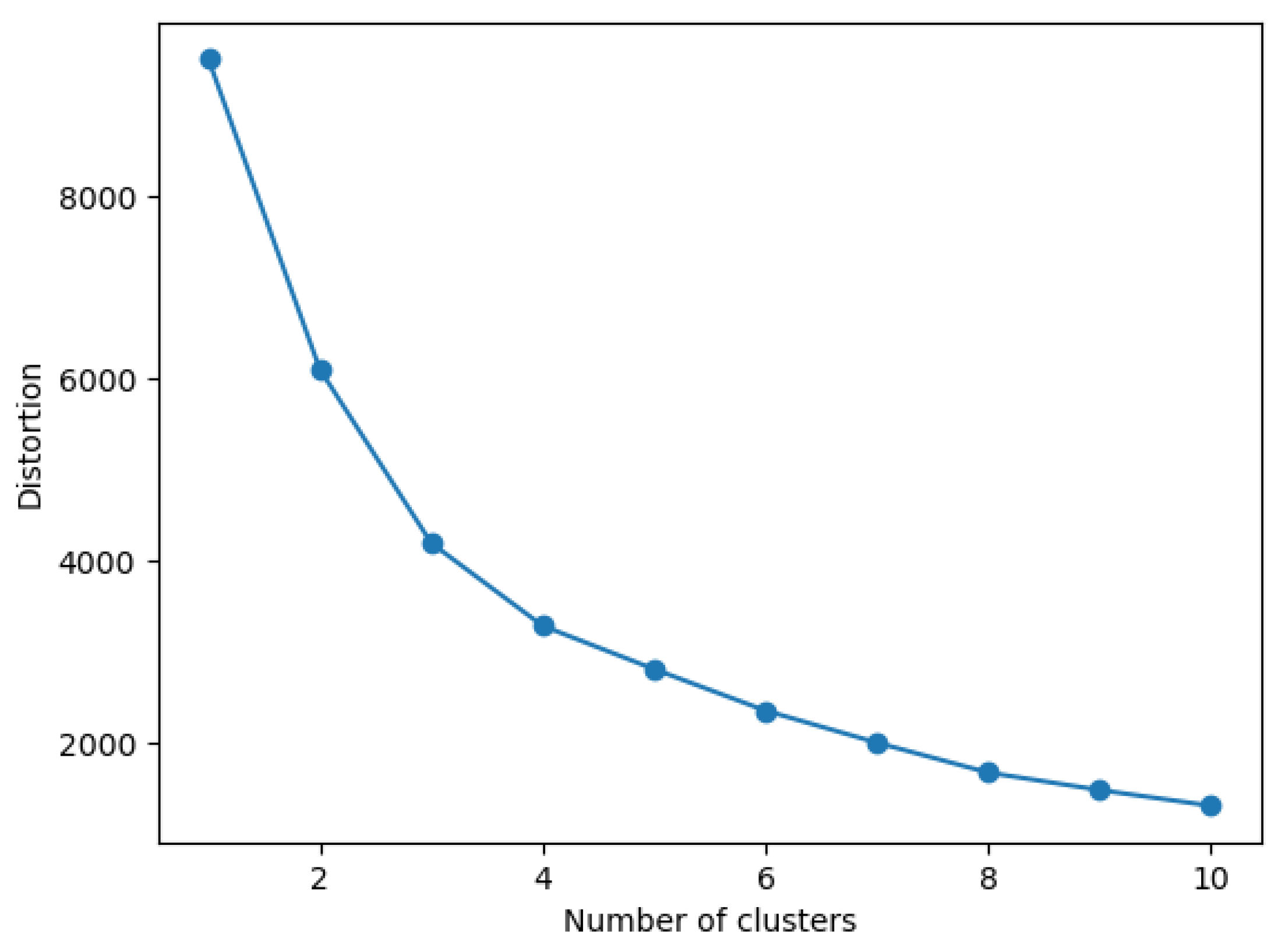
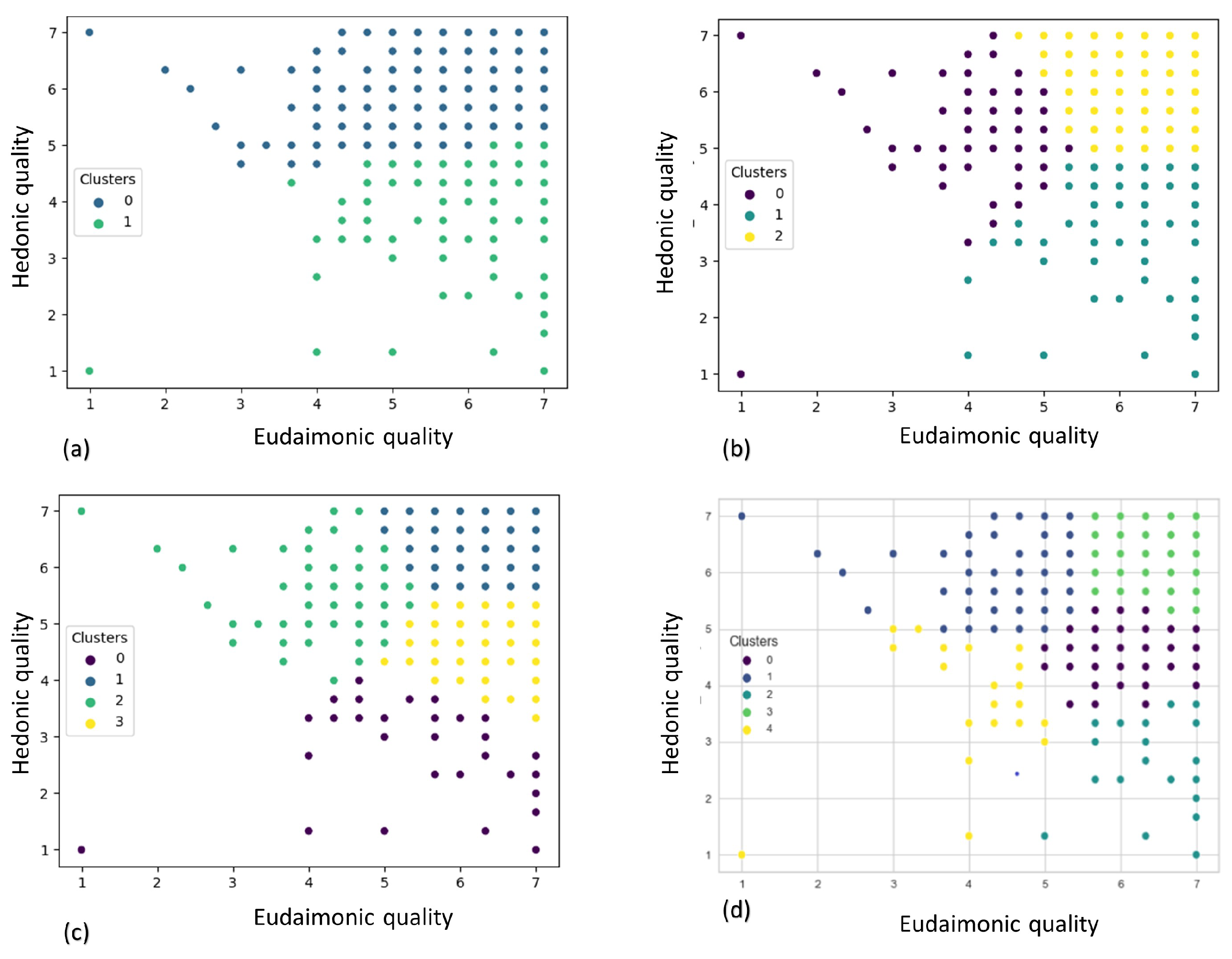
We used the elbow method [31] to determine the optimal number of clusters k, using the KMeans clustering algorithm. Based on the elbow diagram showed in Figure 4, we decided to investigate k values from 2 to 5. The clustering outcome is depicted in Figure 5.
For choosing the best number of clusters we also employed the silhouette method. In this method, the silhouette coefficients are calculated for each data point, which measures the degree of similarity of a data point to its cluster compared to other clusters. The silhouette coefficients can be between −1 to 1. The higher the value of the silhouette coefficient, the more similar the data point is to its cluster than others. A Silhouette coefficient of 1 indicates that the sample is far from other clusters. If the silhouette coefficient is 0, then the sample is close to the decision boundary of two neighboring clusters. If the silhouette coefficient is −1, the sample most likely belongs to another cluster. Silhouette plots are shown in Figure 6.
Based on Figure 6, the average Silhouette coefficient is between 0.3 and 0.4, regardless of k’s value. k = 5 and k = 4 are not good choices, as all samples in one of the clusters are below average Silhouette coefficient. For k = 2, one of the clusters is larger in size than the other one, which gives this intuition that it can be divided into two subclusters. However, outliers emerge for k = 3. For k = 2 and k = 3, we can see silhouette plots and cluster diagrams showing the distribution of clusters in Figure 7. Figure 7 indicates that clusters are more distinguished based on hedonic orientation if we have two clusters (diagram (a)). Eudaimonic orientation impacts the final cluster more if there are three clusters compared to two clusters.
4.2. Eudaimonic and Hedonic Orientation Prediction
The results of EHO prediction are presented as a regression and as a classification problem.
4.2.1. Regression
We evaluated seven machine-learning-regression models. As the baseline, we used the predictor of the mean value of the target variable. We considered two feature sets in the manual feature selection step: (i) U-F features, which contain user-related features (except for EHOQ and EHO variables, which are the target variables) and (ii) I-F features, which describe the users’ interactions. The detailed list of features is reported in Table 1.
To evaluate the prediction of the various algorithms we used the mean absolute error (MAE) and the root mean squared error (RMSE), which penalizes large errors more than MAE [32]. The results are reported in Table 4, Table 5 and Table 6, for feature sets U-F, I-F and both, respectively.
In the regression problem, in the case of using U-F features (Table 4), we can see that Ridge and Lasso performed better compared to the baseline. The SVR also performed better than the baseline based on the MAE and RMSE value in predicting the eudaimonic orientation of users. In terms of hedonic orientation prediction by SVR, only the RMSE value is lower than the baseline. Random Forest and XGBoost provided slightly lower values of RMSE than the baseline but higher MAE values. The decision tree algorithm was only better at predicting hedonic orientation based on the RMSE metric than other methods.
In the regression problem, in the case of using I-F features (Table 5), we can see that the results are more or less close to the baseline, whereas using both U-F and I-F features (Table 6) results are better, except for the MAE value for the KNN algorithm, which is not better but still close to the baseline.
4.2.2. Class Prediction
For the classification problem, the target variables were converted to classes using median splitting. In order to evaluate the classifiers, we used the accuracy, precision, recall, F1 score and the area under the curve (AUC) in the receiver operating characteristic (ROC). Again, we compared U-F and I-F features. As the baseline, we used the majority classifier. Since we used median splitting, the metrics values should be ; however, due to slight inequalities caused by data splitting, they are slightly off the value.
When using the U-F features (Table 7 and Table 8), the Ridge, SVC and Random Forest algorithms performed better than the baseline. The decision tree and KNN performed close but still better than the baseline.
In the classification problem of predicting EO and HO classes using I-F features (Table 9 and Table 10), the Ridge, SVC and Random Forest algorithms performed better than the baseline. The KNN performed close but still better than the baseline. We can see that the decision tree performed better in predicting HO classes than in predicting EO classes.
For most machine-learning algorithms, the results of classification problems using I-F features or U-F features are better than those using the baseline in both cases. When I-F features are used, the decision tree provides better results. With other machine-learning algorithms, the results are close or better than the baseline, regardless of whether I-F or U-F features are used. The baseline performed better in terms of accuracy only when using the decision tree model to predict HO classes using U-F features. For both EO and HO class prediction (Table 11 and Table 12), the Ridge as well as Random Forest algorithms outperformed the baseline significantly.
5. Discussion
A visual inspection of Figure 3 indicates that the users who participated in our user study were mostly users with a high value of eudaimonic characteristics. We are missing norms of the distributions of the EO and HO for the general population to compare our sample with. Such norms do exist for instruments that have been available for a longer time, such as the BFI [33]. We speculate that the participants who decided to take part in our data collection were more film-savvy and hence had high EO. In future work, we would need to collect data with a more representative sample of participants.
We clustered the participants in the space of EO and HO. Based on the elbow method, three to four clusters appear to be a reasonable choice. However, upon inspecting the clusters in the EHO space, three clusters seems better as the users are nicely separated according to their orientations. In fact, looking at Figure 5b, we can see that cluster 0 is formed of people with low eudaimonic orientation but high hedonic orientation (pleasure seekers). Cluster 1 is characterized by low HO and high EU (meaning seekers). Finally, the users in cluster 2 exhibit both high EO and high HO, which is a novel cluster compared to our previous work [14].
In terms of which ML algorithm is the best for the task at hand, the ridge and lasso regressors and the ridge classifier appears to yield the best results across different setups. There are differences in the performance due to various feature sets but these algorithms constantly outperform others independently on the feature sets, the target variable and the metric.
Generally, the U-F set yields better prediction performance than the I-F set of features. However, the results show that the metric used accounts for how much the features improve over the baseline. When using the U-F features only, there is a substantial improvement both in the RMSE and MAE in both target variables compared to the baseline. When using the I-F features, however, the difference is smaller. Furthermore, in terms of the MAE, the difference is almost negligible, while in terms of the RMSE there is a stronger improvement of prediction over the baseline.
In the classification problem, the different metrics used (accuracy, precision, recall, F-score and area under curve) show different aspects of the classifier performance. However, in our case, accuracy and precision are the most important. Although, here, the U-F features again perform better than the I-F features, the difference is not as pronounced as in the regression case. It is clear that both sets of features account for a substantial amount of variance in HO and EO of users.
6. Conclusions
In this paper, we presented the experimental results of a machine-learning model that predicts the eudaimonic and hedonic orientation of users in the domain of movies. We proposed an approach where features are extracted from user preferences for movies and demographic characteristics, which is a typical set of information present in movie recommender systems. We evaluated the proposed approach on a moderate-sized dataset of 350 users and 703 movies and showed that understanding the hedonic and eudaimonic characteristics of movies and user preferences are good indicators of the eudaimonic and hedonic orientations of users.
Based on the research questions, we showed that (i) There were no distinct clusters of users in the EO-HO space. However, the elbow method indicated that three clusters appears to be a reasonable interpretation: (a) users with high HO and EO, (b) users with high HO and low EO and (c) users with low HO and high HO. Furthermore, we showed that, on our dataset, (ii) the ridge and lasso regressors and the ridge classifier performed the best across a range of different feature sets and metrics. Finally, we showed that (iii) I-F features improved the prediction over the baseline, both in regression and classification; however, the major boost was given by the U-F features.
Future work should address the issue of the potentially non-representative sample. Furthermore, other domains than movies should be explored—for example, music and books. We also plan to examine the performance of predicting the eudaimonic/hedonic qualities of movies from their subtitles using state-of-the-art algorithms, such as support vector machines, convolution neural networks, recurrent neural networks and Bert [34]. Finally, the proposed approach should be integrated into a recommender system pipeline to evaluate how much the proposed approach helps in improving the quality of recommendations.
Author Contributions
Conceptualization, E.M. and M.T.; methodology, E.M., F.B. and M.T.; software, E.M.; validation, E.M., F.B. and M.T.; formal analysis, E.M.; investigation, E.M., F.B. and M.T.; resources, E.M.; data curation, E.M.; writing—original draft preparation, E.M.; writing—review and editing, E.M., F.B. and M.T.; visualization, E.M.; supervision, M.T.; project administration, M.T.; funding acquisition, M.T. All authors have read and agreed to the published version of the manuscript.
Funding
This research received no external funding.
Informed Consent Statement
Informed consent was obtained from all subjects involved in the study.
Data Availability Statement
Data are available at the corresponding author upon written request.
Conflicts of Interest
The authors declare no conflict of interest.
Abbreviations
The following abbreviations are used in this manuscript:
| BFI | Big Five Inventory |
| EHO | eudaimonic and hedonic orientation of users |
| EO | eudaimonic orientation of users |
| HO | hedonic orientation of users |
| EHP | eudaimonic and hoedonic perception of users |
| EP | eudaimonic perception of users |
| HP | hedonic perception of users |
| FFM | Five Factor Model |
| MSI | Musical Sophistication Index |
| TIPI | Ten-Item Personality Inventory |
References
- McCrae, R.R.; John, O.P. An Introduction to the Five-Factor Model and its Applications. J. Personal. 1992, 60, 175–215. [Google Scholar] [CrossRef] [PubMed]
- Tkalčič, M.; Chen, L. Personality and Recommender Systems. In Recommender Systems Handbook; Ricci, F., Rokach, L., Shapira, B., Eds.; Springer: New York, NY, USA, 2022; pp. 757–787. [Google Scholar] [CrossRef]
- Matz, S.C.; Kosinski, M.; Nave, G.; Stillwell, D.J. Psychological targeting as an effective approach to digital mass persuasion. Proc. Natl. Acad. Sci. USA 2017, 114, 12714–12719. [Google Scholar] [CrossRef] [PubMed]
- Quercia, D.; Kosinski, M.; Stillwell, D.; Crowcroft, J. Our twitter profiles, our selves: Predicting personality with twitter. In Proceedings of the 2011 IEEE International Conference on Privacy, Security, Risk and Trust and IEEE International Conference on Social Computing, PASSAT/SocialCom 2011, Boston, MA, USA, 9–11 October 2011; pp. 180–185. [Google Scholar] [CrossRef]
- Golbeck, J.; Robles, C.; Edmondson, M.; Turner, K. Predicting Personality from Twitter. In Proceedings of the 2011 IEEE Third Int’l Conference on Privacy, Security, Risk and Trust and 2011 IEEE Third Int’l Conference on Social Computing, Boston, MA, USA, 9–11 October 2011; pp. 149–156. [Google Scholar] [CrossRef]
- Kosinski, M.; Stillwell, D.; Graepel, T. Private traits and attributes are predictable from digital records of human behavior. Proc. Natl. Acad. Sci. USA 2013, 110, 5802–5805. [Google Scholar] [CrossRef] [PubMed]
- Skowron, M.; Tkalčič, M.; Ferwerda, B.; Schedl, M. Fusing Social Media Cues. In Proceedings of the 25th International Conference Companion on World Wide Web-WWW ’16 Companion, Montréal, QC, Canada, 11–15 May 2016; ACM Press: New York, NY, USA, 2016; pp. 107–108. [Google Scholar] [CrossRef]
- Azucar, D.; Marengo, D.; Settanni, M. Predicting the Big 5 personality traits from digital footprints on social media: A meta-analysis. Personal. Individ. Differ. 2018, 124, 150–159. [Google Scholar] [CrossRef]
- Matz, S.; Chan, Y.W.F.; Kosinski, M. Models of Personality. In Emotions and Personality in Personalized Services: Models, Evaluation and Applications; Tkalčič, M., De Carolis, B., de Gemmis, M., Odić, A., Košir, A., Eds.; Springer International Publishing: Cham, Switzerland, 2016; pp. 35–54. [Google Scholar] [CrossRef]
- Stewart, B. Personality and Play Styles: A Unified Model. 2011, pp. 1–11. Available online: https://mud.co.uk/richard/hcds.htm (accessed on 15 September 2022).
- Holland, J.L. Making Vocational Choices: A Theory of Vocational Personalities and Work Environments; Psychological Assessment Resources; PrenticeHall: Englewood Cliffs, NJ, USA, 1997; Volume 3, pp. XIV, 303 S. [Google Scholar]
- Thomas, K.W.; Kilmann, R.H.; Trainer, J. Thomas–Kilmann Conflict Mode Instrument COMPETING ASSERTIVENESS; US, Jane Trainer Acme: Belmont, CA, USA, 2010. [Google Scholar]
- Oliver, M.B.; Raney, A.A. Entertainment as Pleasurable and Meaningful: Identifying Hedonic and Eudaimonic Motivations for Entertainment Consumption. J. Commun. 2011, 61, 984–1004. [Google Scholar] [CrossRef]
- Tkalčič, M.; Ferwerda, B. Eudaimonic Modeling of Moviegoers. In Proceedings of the 26th Conference on User Modeling, Adaptation and Personalization, Singapore, 8–11 July 2018; ACM: New York, NY, USA, 2018; pp. 163–167. [Google Scholar] [CrossRef]
- Tkalcic, M.; Motamedi, E.; Barile, F.; Puc, E.; Mars Bitenc, U. Prediction of Hedonic and Eudaimonic Characteristics from User Interactions. In Proceedings of the Adjunct Proceedings of the 30th ACM Conference on User Modeling, Adaptation and Personalization, Barcelona, Spain, 4–7 July 2022; ACM: Barcelona, Spain, 2022; pp. 366–370. [Google Scholar] [CrossRef]
- Allport, G.W. Concepts of trait and personality. Psychol. Bull. 1927, 24, 284. [Google Scholar] [CrossRef]
- Goldberg, L.R. An alternative “description of personality”: The big-five factor structure. J. Personal. Soc. Psychol. 1990, 59, 1216. [Google Scholar] [CrossRef]
- Fiske, D.W. Consistency of the factorial structures of personality ratings from different sources. J. Abnorm. Soc. Psychol. 1949, 44, 329. [Google Scholar] [CrossRef] [PubMed]
- Feher, A.; Vernon, P.A. Looking beyond the Big Five: A selective review of alternatives to the Big Five model of personality. Personal. Individ. Differ. 2021, 169, 110002. [Google Scholar] [CrossRef]
- Delic, A.; Neidhardt, J.; Nguyen, T.N.; Ricci, F. An observational user study for group recommender systems in the tourism domain. Inf. Technol. Tour. 2018, 19, 87–116. [Google Scholar] [CrossRef]
- Abolghasemi, R.; Engelstad, P.; Herrera-Viedma, E.; Yazidi, A. A personality-aware group recommendation system based on pairwise preferences. Inf. Sci. 2022, 595, 1–17. [Google Scholar] [CrossRef]
- Botella, C.; Riva, G.; Gaggioli, A.; Wiederhold, B.K.; Alcaniz, M.; Baños, R.M.; Erino, S.I.S.; Ipresso, P.I.C.; Aggioli, A.N.G.; Allavicini, F.E.P.; et al. The Present and Future of Positive Technologies. Cyberpsychol. Behav. Soc. Netw. 2012, 15, 78–84. [Google Scholar] [CrossRef] [PubMed]
- Wirth, W.; Hofer, M.; Schramm, H. Beyond Pleasure: Exploring the Eudaimonic Entertainment Experience. Hum. Commun. Res. 2012, 38, 406–428. [Google Scholar] [CrossRef]
- John, O.; Srivastava, S. The Big Five trait taxonomy: History, measurement, and theoretical perspectives. In Handbook of Personality: Theory and Research, 2nd ed.; Pervin, L.A., John, O.P., Eds.; Guilford Press: New York, NY, USA, 1999; Volume 2, pp. 102–138. [Google Scholar]
- Ferwerda, B.; Tkalčič, M. You Are What You Post: What the Content of Instagram Pictures Tells About Users’ Personality. In Proceedings of the ACM IUI 2018 Workshops, Tokyo, Japan, 7–11 March 2018; Volume 2068. [Google Scholar]
- Ferwerda, B.; Tkalčič, M. Exploring the Prediction of Personality Traits from Drug Consumption Profiles. In Proceedings of the Adjunct Publication of the 28th ACM Conference on User Modeling, Adaptation and Personalization, Genoa, Italy, 12–18 July 2020; ACM: Genoa, Italy, 2020; pp. 2–5. [Google Scholar] [CrossRef]
- Berkovsky, S.; Taib, R.; Koprinska, I.; Wang, E.; Zeng, Y.; Li, J.; Kleitman, S. Detecting Personality Traits Using Eye-Tracking Data. In Proceedings of the 2019 CHI Conference on Human Factors in Computing Systems-CHI ’19, Glasgow, UK, 4–9 May 2019; pp. 1–12. [Google Scholar] [CrossRef]
- Gosling, S.D.; Rentfrow, P.J.; Swann, W.B., Jr. A very brief measure of the Big-Five personality domains. J. Res. Personal. 2003, 37, 504–528. [Google Scholar] [CrossRef]
- Müllensiefen, D.; Gingras, B.; Musil, J.; Stewart, L. The musicality of non-musicians: An index for assessing musical sophistication in the general population. PLoS ONE 2014, 9, e89642. [Google Scholar] [CrossRef] [PubMed]
- Van Rijn, J.N.; Hutter, F. Hyperparameter importance across datasets. In Proceedings of the 24th ACM SIGKDD International Conference on Knowledge Discovery & Data Mining, London, UK, 19–23 August 2018; pp. 2367–2376. [Google Scholar]
- Nainggolan, R.; Perangin-angin, R.; Simarmata, E.; Tarigan, A.F. Improved the performance of the K-means cluster using the sum of squared error (SSE) optimized by using the Elbow method. J. Phys. Conf. Ser. 2019, 1361, 012015. [Google Scholar] [CrossRef]
- Dou, Z.; Sun, Y.; Zhang, Y.; Wang, T.; Wu, C.; Fan, S. Regional Manufacturing Industry Demand Forecasting: A Deep Learning Approach. Appl. Sci. 2021, 11, 6199. [Google Scholar] [CrossRef]
- Srivastava, S. Norms for the Big Five Inventory and other personality measures. Hardest Sci. 2012, 17. Available online: https://thehardestscience.com/2012/10/17/norms-for-the-big-five-inventory-and-other-personality-measures/ (accessed on 15 September 2022).
- Hu, Y.; Ding, J.; Dou, Z.; Chang, H. Short-text classification detector: A bert-based mental approach. Comput. Intell. Neurosci. 2022, 2022, 8660828. [Google Scholar] [CrossRef] [PubMed]
Figure 1.
The machine-learning pipeline (symbols with dashed line edges illustrate that that step is not always performed).
Figure 1.
The machine-learning pipeline (symbols with dashed line edges illustrate that that step is not always performed).

Figure 2.
The machine-learning pipeline in more details (symbols with dashed line edges illustrate that that step is not always performed).
Figure 2.
The machine-learning pipeline in more details (symbols with dashed line edges illustrate that that step is not always performed).

Figure 3.
The distribution of users: (a) histogram of hedonic (blue) and eudaimonic (green) values and (b) eudaimonic vs. hedonic quality.
Figure 3.
The distribution of users: (a) histogram of hedonic (blue) and eudaimonic (green) values and (b) eudaimonic vs. hedonic quality.

Figure 4.
Elbow diagram. x-axis = Number of clusters; y-axis = Distortion (sum of square errors) of data points in the clusters. The clustering was performed with KMeans over eudaimonic and hedonic variables.
Figure 4.
Elbow diagram. x-axis = Number of clusters; y-axis = Distortion (sum of square errors) of data points in the clusters. The clustering was performed with KMeans over eudaimonic and hedonic variables.

Figure 5.
Different clusters formed by KMeans over eudaimonic and hedonic variables. (a): k = 2, (b): k = 3, (c): k = 4 and (d): k = 5. The parameter k of KMeans in scikit-learn library determines the number of clusters.
Figure 5.
Different clusters formed by KMeans over eudaimonic and hedonic variables. (a): k = 2, (b): k = 3, (c): k = 4 and (d): k = 5. The parameter k of KMeans in scikit-learn library determines the number of clusters.

Figure 6.
The different number of clusters using the silhouette method over eudaimonic and hedonic variables. (a): k = 2, (b): k = 3, (c): k = 4 and (d): k = 5. Parameter k determines the number of clusters. The average value of the Silhouette coefficients is shown with a red dashed line.
Figure 6.
The different number of clusters using the silhouette method over eudaimonic and hedonic variables. (a): k = 2, (b): k = 3, (c): k = 4 and (d): k = 5. Parameter k determines the number of clusters. The average value of the Silhouette coefficients is shown with a red dashed line.

Figure 7.
The different number of clusters using silhouette method over eudaimonic and hedonic variables. (a): number of clusters = 2 and (b): number of clusters = 3. Parameter n_clusters determines the number of clusters. The average value of the Silhouette coefficients is shown with a red dashed line.


Table 1.
Feature list. Answers to the question sets provided to users are represented by feature groups ending in Q. BFT, EHO and SFI were calculated based on user responses. The features that describe users and interactions are U-F and I-F, respectively.
Table 1.
Feature list. Answers to the question sets provided to users are represented by feature groups ending in Q. BFT, EHO and SFI were calculated based on user responses. The features that describe users and interactions are U-F and I-F, respectively.
| Feature Groups | Feature Subgroups | Description | Range of Values |
|---|---|---|---|
| U-F | DEMQ | Demographic questions (ie: gender, education and age) | Age > 18 Others: categorical features |
| GPREFQ | Genre preference questions (including: action, adventure, comedy, drama, fantasy, history, romance, science fiction, thriller) | 5 likert scale | |
| BFIQ | Big five inventory questions | 7 likert scale | |
| EHOQ | Eudaimonic and hedonic orientation questions | 7 likert scale | |
| SFIQ | Sophisticaiton index questions | 7 likert scale | |
| BFT | Big five traits (calculated from BFIQ) | ||
| EHO | Eudaimonic and hedonic orientation of users (calculated from EHOQ) | ||
| SFI | sophistication indexes including: active engagement, emotion (calculated from SFIQ) | ||
| I-F | FPREFQ | Film preference questions | 5 likert scale |
| EHPQ | Questions related to eudaimonic and hedonic perceptions of users from films | 7 likert scale | |
| EHP | Eudaimonic and hedonic perceptions of users from films (calculated from EHPQ) |
Table 2.
ML models and hyperparameters (regression problem). Except for XGBRegressor, Scikit-learn was used to implement all models (https://scikit-learn.org/stable/ accessed on 15 September 2022). Python’s xgboost library was used to implement XGBRegressor. (https://xgboost.readthedocs.io/en/stable/parameter.html accessed on 15 September 2022).
| Model | Scaled | Parameters | Tested Values |
|---|---|---|---|
| Ridge | ✓ | alpha (regularization parameter) | 0, 0.0001, 0.001, 0.01, 0.1, 1, 5, 10 |
| Lasso | ✓ | alpha (regularization parameter) | 0, 0.0001, 0.001, 0.01, 0.1, 1, 5, 10 |
| SVR | ✓ | Kernel | linear, rbf, poly |
| C | 0.001, 0.01, 0.1, 1.0, 10, 100 | ||
| gamma | scale, auto | ||
| epsilon | 0.001, 0.01, 0.1, 0.2, 0.5, 0.3, 1.0, 2.0, 4.0 | ||
| KNeighborsRegressor | ✓ | n_neighbors | 3, 5, 7, 9 |
| weights | uniform, distance | ||
| algorithm | ball_tree, kd_tree, brute | ||
| p | 1, 2 | ||
| DecisionTreeRegressor | X | criterion | mae, mse |
| splitter | best, random | ||
| max_depth | 1, 3, 5, 7, 9, 11, 12 | ||
| min_weight_fraction_leaf | 0.1, 0.2, 0.3, 0.4, 0.5 | ||
| max_features | auto, log2, sqrt, None | ||
| max_leaf_nodes | None, 10, 20, 30, 40, 50, 60, 70, 80, 90 | ||
| RandomForestRegressor | X | n_estimators | 1, 3, 5, 7, 9, 11, 13, 15, 17, 20 |
| max_features | auto, sqrt | ||
| max_depth | 1, 3, 5, 7, 9, 11, 13, 15, 17, 20 | ||
| min_samples_split | 2, 3, 4, 5, 10 | ||
| min_samples_leaf | 1, 2, 4 | ||
| bootstrap | True, False | ||
| XGBRegressor | X | max_depth | 3, 4, 5, 6, 7, 8, 9, 10, 11 |
| min_child_weight | 1, 2, 3, 4, 5, 6, 7 | ||
| eta | 0.001, 0.01, 0.1, 0.2, 0.5, 0.3, 1 | ||
| subsample | 0.7, 0.8, 0.9, 1.0 | ||
| colsample_bytree | 0.7, 0.8, 0.9, 1.0 | ||
| objective | reg:squarederror |
Table 3.
ML models and hyperparameters (classification problem). Except for XGBRegressor, Scikit-learn was used to implement all models (https://scikit-learn.org/stable/, accessed on 15 September 2022). Python’s xgboost library was used to implement XGBRegressor. (https://xgboost.readthedocs.io/en/stable/parameter.html, accessed on 15 September 2022).
| Model | Scaled | Parameters | Tested Values |
|---|---|---|---|
| Ridge | ✓ | alpha (regularization parameter) | 0, 0.0001, 0.001, 0.01, 0.1, 1, 5, 10 |
| SVC | ✓ | Kernel | linear, rbf, poly |
| C | 0.001, 0.01, 0.1, 1.0, 10, 100 | ||
| gamma | 0.001, 0.01, 0.1, 1 | ||
| KNeighborsClassifier | ✓ | n_neighbors | 3, 5, 7, 9 |
| weights | uniform, distance | ||
| algorithm | ball_tree, kd_tree, brute | ||
| p | 1, 2 | ||
| DecisionTreeClassifier | X | criterion | gini, entropy |
| splitter | best, random | ||
| max_depth | 1, 3, 5, 7, 9, 11, 12 | ||
| min_weight_fraction_leaf | 0.1, 0.2, 0.3, 0.4, 0.5 | ||
| max_features | auto, log2, sqrt, None | ||
| max_leaf_nodes | None, 10, 20, 30, 40, 50, 60, 70, 80, 90 | ||
| RandomForestClassifier | X | n_estimators | 1, 5, 9, 13, 17, 20 |
| max_depth | 1, 5, 9, 13, 17, 20 | ||
| min_samples_split | 2, 3, 4, 5, 10 | ||
| min_samples_leaf | 1, 2, 4 | ||
| bootstrap | True, False | ||
| XGBClassifier | X | max_depth | 3, 4, 5, 6, 7, 8, 9, 10, 11 |
| min_child_weight | 1, 2, 3, 4, 5, 6, 7 | ||
| eta | 0.001, 0.01, 0.1, 0.2, 0.5, 0.3, 1 | ||
| subsample | 0.7, 0.8, 0.9, 1.0 | ||
| colsample_bytree | 0.7, 0.8, 0.9, 1.0 | ||
| objective | reg:squarederror |
Table 4.
EHO prediction results (regression problem) using U-F features. Nested cross-validation with 10 outer and five inner splits. EO (Eudaimonic orientation) and HO (Hedonic orientation). Numbers are the mean value of 10 outer splits. Numbers in parenthesis indicate the standard deviation values.
| ML Algorithm | RMSE (EO) | MAE (EO) | RMSE (HO) | MAE (HO) |
|---|---|---|---|---|
| Base | 1.09 (0.00) | 0.85 (0.00) | 1.24 (0.00) | 0.97 (0.00) |
| Ridge | 0.88 (0.07) | 0.48 (0.07) | 1.02 (0.07) | 0.86 (0.10) |
| Lasso | 0.88 (0.06) | 0.48 (0.07) | 1.02 (0.07) | 0.86 (0.11) |
| SVR | 0.96 (0.10) | 0.66 (0.11) | 1.10 (0.09) | 1.17 (0.17) |
| KNN | 1.07 (0.09) | 1.01 (0.15) | 1.11 (0.08) | 1.14 (0.16) |
| Decision Tree | 1.09 (0.10) | 1.06 (0.15) | 1.15 (0.08) | 1.37 (0.21) |
| Random Forest | 1.07 (0.09) | 1.00 (0.17) | 1.09 (0.11) | 1.09 (0.19) |
| XGBoost | 1.06 (0.15) | 0.98 (0.26) | 1.08 (0.07) | 1.05 (0.13) |
Table 5.
EHO prediction results (regression problem) using I-F features. Nested cross-validation with 10 outer and five inner splits. EO (Eudaimonic orientation) and HO (Hedonic orientation). Numbers are the mean value of 10 outer splits. Numbers in parenthesis indicate the standard deviation values.
| ML Algorithm | RMSE (EO) | MAE (EO) | RMSE (HO) | MAE (HO) |
|---|---|---|---|---|
| Base | 1.09 (0.00) | 0.85 (0.00) | 1.24 (0.00) | 0.97 (0.00) |
| Ridge | 1.02 (0.09) | 0.87 (0.12) | 1.04 (0.08) | 0.94 (0.12) |
| Lasso | 1.02 (0.09) | 0.86 (0.12) | 1.05 (0.07) | 0.94 (0.11) |
| SVR | 1.04 (0.09) | 0.92 (0.13) | 1.07 (0.09) | 1.01 (0.15) |
| KNN | 1.05 (0.10) | 0.95 (0.14) | 1.10 (0.10) | 1.16 (0.18) |
| Decision Tree | 1.08 (0.11) | 1.06 (0.18) | 1.10 (0.08) | 1.15 (0.15) |
| Random Forest | 1.06 (0.11) | 0.99 (0.15) | 1.10 (0.09) | 1.15 (0.17) |
| XGBoost | 1.07 (0.12) | 1.03 (0.19) | 1.09 (0.09) | 1.09 (0.16) |
Table 6.
EHO prediction results (regression problem) using U-F and I-F features. Nested cross-validation with 10 outer and five inner splits. EO (Eudaimonic orientation) and HO (Hedonic orientation). Numbers are the mean value of 10 outer splits. Numbers in parenthesis indicate the standard deviation values.
| ML Algorithm | RMSE (EO) | MAE (EO) | RMSE (HO) | MAE (HO) |
|---|---|---|---|---|
| Base | 1.09 (0.00) | 0.85 (0.00) | 1.24 (0.00) | 0.97 (0.00) |
| Ridge | 0.88 (0.04) | 0.48 (0.05) | 1.03 (0.04) | 0.87 (0.07) |
| Lasso | 0.87 (0.05) | 0.47 (0.05) | 1.02 (0.05) | 0.86 (0.07) |
| SVR | 0.97 (0.07) | 0.69 (0.06) | 1.02 (0.05) | 0.86 (0.08) |
| KNN | 1.04 (0.08) | 0.90 (0.10) | 1.05 (0.04) | 0.95 (0.08) |
| Decision Tree | 1.01 (0.07) | 0.82 (0.08) | 1.05 (0.06) | 0.93 (0.09) |
| Random Forest | 1.01 (0.06) | 0.82 (0.08) | 1.04 (0.07) | 0.90 (0.11) |
| XGBoost | 0.98 (0.04) | 0.74 (0.06) | 1.04 (0.07) | 0.89 (0.10) |
Table 7.
EO prediction results (classification problem) using U-F features. Nested cross-validation with 10 outer and five inner splits. Classification problems on two classes: (a): High_EO (High Eudaimonic Orientated) and (b): Low_EO (Low Eudaimonic Oriented). Numbers are the mean value of 10 outer splits. Numbers in parenthesis indicate the standard deviation values.
| ML Algorithm | Accuracy | Precision | Recall | F1 Score | ROC AUC |
|---|---|---|---|---|---|
| Base | 0.51 (0.00) | 0.00 (0.00) | 0.00 (0.00) | 0.00 (0.00) | 0.50 (0.00) |
| Ridge | 0.78 (0.08) | 0.75 (0.12) | 0.86 (0.12) | 0.79 (0.08) | 0.89 (0.07) |
| SVC | 0.65 (0.07) | 0.66 (0.09) | 0.61 (0.12) | 0.63 (0.08) | 0.71 (0.08) |
| KNN | 0.57 (0.11) | 0.57 (0.15) | 0.55 (0.15) | 0.55 (0.13) | 0.60 (0.10) |
| Decision Tree | 0.53 (0.11) | 0.53 (0.13) | 0.53 (0.13) | 0.52 (0.12) | 0.52 (0.11) |
| Random Forest | 0.62 (0.08) | 0.62 (0.09) | 0.58 (0.09) | 0.60 (0.07) | 0.68 (0.08) |
Table 8.
HO prediction results (classification problem) using U-F features. Nested cross-validation with 10 outer and five inner splits. Classification problems on two classes: (a): High_HO (High Hedonic Orientated) and (b): Low_HO (Low Hedonic Oriented). Numbers are the mean value of 10 outer splits. Numbers in parenthesis indicate the standard deviation values.
| ML Algorithm | Accuracy | Precision | Recall | F1 Score | ROC AUC |
|---|---|---|---|---|---|
| Base | 0.56 (0.00) | 0.00 (0.00) | 0.00 (0.00) | 0.00 (0.00) | 0.50 (0.00) |
| Ridge | 0.66 (0.07) | 0.63 (0.10) | 0.63 (0.11) | 0.62 (0.05) | 0.72 (0.07) |
| SVC | 0.65 (0.07) | 0.60 (0.13) | 0.61 (0.15) | 0.60 (0.12) | 0.69 (0.10) |
| KNN | 0.59 (0.08) | 0.55 (0.15) | 0.48 (0.08) | 0.51 (0.10) | 0.60 (0.09) |
| Decision Tree | 0.53 (0.11) | 0.53 (0.13) | 0.53 (0.13) | 0.52 (0.12) | 0.52 (0.11) |
| Random Forest | 0.63 (0.06) | 0.63 (0.15) | 0.52 (0.12) | 0.54 (0.10) | 0.65 (0.06) |
Table 9.
EO prediction results (classification problem) using I-F features. Nested cross-validation with 10 outer and five inner splits. Classification problems on two classes: (a): High_EO (High Eudaimonic Orientated) and (b): Low_EO (Low Eudaimonic Oriented). Numbers are the mean value of 10 outer splits. Numbers in parenthesis indicate the standard deviation values.
| ML Algorithm | Accuracy | Precision | Recall | F1 Score | ROC AUC |
|---|---|---|---|---|---|
| Base | 0.51 (0.00) | 0.00 (0.00) | 0.00 (0.00) | 0.00 (0.00) | 0.50 (0.00) |
| Ridge | 0.56 (0.02) | 0.56 (0.04) | 0.54 (0.04) | 0.55 (0.01) | 0.59 (0.02) |
| SVC | 0.60 (0.03) | 0.60 (0.03) | 0.58 (0.05) | 0.59 (0.02) | 0.63 (0.03) |
| KNN | 0.57 (0.04) | 0.57 (0.04) | 0.55 (0.05) | 0.56 (0.04) | 0.60 (0.04) |
| Decision Tree | 0.62 (0.04) | 0.61 (0.05) | 0.61 (0.06) | 0.61 (0.05) | 0.64 (0.06) |
| Random Forest | 0.61 (0.06) | 0.60 (0.06) | 0.61 (0.06) | 0.60 (0.05) | 0.66 (0.07) |
Table 10.
HO prediction results (classification problem) using I-F features. Nested cross-validation with 10 outer and five inner splits. Classification problems on two classes: (a): High_HO (High Hedonic Orientated) and (b): Low_HO (Low Hedonic Oriented). Numbers are the mean value of 10 outer splits. Numbers in parenthesis indicate the standard deviation values.
| ML Algorithm | Accuracy | Precision | Recall | F1 Score | ROC AUC |
|---|---|---|---|---|---|
| Base | 0.56 (0.00) | 0.00 (0.00) | 0.00 (0.00) | 0.00 (0.00) | 0.50 (0.00) |
| Ridge | 0.61 (0.03) | 0.56 (0.04) | 0.54 (0.05) | 0.55 (0.03) | 0.65 (0.03) |
| SVC | 0.63 (0.02) | 0.60 (0.04) | 0.53 (0.04) | 0.56 (0.03) | 0.69 (0.02) |
| KNN | 0.63 (0.03) | 0.59 (0.07) | 0.53 (0.04) | 0.56 (0.04) | 0.67 (0.04) |
| Decision Tree | 0.66 (0.04) | 0.63 (0.06) | 0.59 (0.10) | 0.60 (0.06) | 0.72 (0.06) |
| Random Forest | 0.65 (0.06) | 0.62 (0.07) | 0.56 (0.07) | 0.59 (0.07) | 0.70 (0.06) |
Table 11.
EO prediction results (classification problem) using I-F and U-F features. Nested cross-validation with 10 outer and five inner splits. Classification problems on two classes: (a): High_EO (High Eudaimonic Orientated) and (b): Low_EO (Low Eudaimonic Oriented). Numbers are the mean value of 10 outer splits. Numbers in parenthesis indicate the standard deviation values.
| ML Algorithm | Accuracy | Precision | Recall | F1 Score | ROC AUC |
|---|---|---|---|---|---|
| Base | 0.51 (0.00) | 0.00 (0.00) | 0.00 (0.00) | 0.00 (0.00) | 0.50 (0.00) |
| Ridge | 0.77 (0.08) | 0.73 (0.08) | 0.83 (0.13) | 0.77 (0.09) | 0.85 (0.08) |
| SVC | 0.55 (0.09) | 0.54 (0.16) | 0.46 (0.17) | 0.49 (0.15) | 0.58 (0.12) |
| KNN | 0.50 (0.07) | 0.50 (0.09) | 0.47 (0.09) | 0.48 (0.08) | 0.51 (0.07) |
| Decision Tree | 0.55 (0.09) | 0.54 (0.14) | 0.58 (0.11) | 0.55 (0.11) | 0.55 (0.10) |
| Random Forest | 0.64 (0.06) | 0.63 (0.10) | 0.64 (0.10) | 0.63 (0.08) | 0.70 (0.08) |
Table 12.
HO prediction results (classification problem) using I-F and U-F features. Nested cross-validation with 10 outer and five inner splits. Classification problems on two classes: (a): High_HO (High Hedonic Orientated) and (b): Low_HO (Low Hedonic Oriented). Numbers are the mean value of 10 outer splits. Numbers in parenthesis indicate the standard deviation values.
| ML Algorithm | Accuracy | Precision | Recall | F1 Score | ROC AUC |
|---|---|---|---|---|---|
| Base | 0.56 (0.00) | 0.00 (0.00) | 0.00 (0.00) | 0.00 (0.00) | 0.50 (0.00) |
| Ridge | 0.65 (0.06) | 0.62 (0.14) | 0.60 (0.09) | 0.59 (0.07) | 0.70 (0.07) |
| SVC | 0.55 (0.07) | 0.50 (0.15) | 0.46 (0.08) | 0.47 (0.09) | 0.56 (0.08) |
| KNN | 0.54 (0.09) | 0.49 (0.16) | 0.49 (0.14) | 0.48 (0.13) | 0.54 (0.10) |
| Decision Tree | 0.61 (0.06) | 0.58 (0.16) | 0.59 (0.11) | 0.56 (0.07) | 0.62 (0.07) |
| Random Forest | 0.64 (0.07) | 0.61 (0.18) | 0.53 (0.11) | 0.56 (0.12) | 0.68 (0.06) |
Publisher’s Note: MDPI stays neutral with regard to jurisdictional claims in published maps and institutional affiliations. |
© 2022 by the authors. Licensee MDPI, Basel, Switzerland. This article is an open access article distributed under the terms and conditions of the Creative Commons Attribution (CC BY) license (https://creativecommons.org/licenses/by/4.0/).
Share and Cite
MDPI and ACS Style
Motamedi, E.; Barile, F.; Tkalčič, M. Prediction of Eudaimonic and Hedonic Orientation of Movie Watchers. Appl. Sci. 2022, 12, 9500. https://0-doi-org.brum.beds.ac.uk/10.3390/app12199500
AMA Style
Motamedi E, Barile F, Tkalčič M. Prediction of Eudaimonic and Hedonic Orientation of Movie Watchers. Applied Sciences. 2022; 12(19):9500. https://0-doi-org.brum.beds.ac.uk/10.3390/app12199500
Chicago/Turabian StyleMotamedi, Elham, Francesco Barile, and Marko Tkalčič. 2022. "Prediction of Eudaimonic and Hedonic Orientation of Movie Watchers" Applied Sciences 12, no. 19: 9500. https://0-doi-org.brum.beds.ac.uk/10.3390/app12199500
Note that from the first issue of 2016, this journal uses article numbers instead of page numbers. See further details here.