Optimal Defense Strategy Selection Algorithm Based on Reinforcement Learning and Opposition-Based Learning

Abstract

Industrial control systems (ICS) are facing increasing cybersecurity issues, leading to enormous threats and risks to numerous industrial infrastructures. In order to resist such threats and risks, it is particularly important to scientifically construct security strategies before an attack occurs. The characteristics of evolutionary algorithms are very suitable for finding optimal strategies. However, the more common evolutionary algorithms currently used have relatively large limitations in convergence accuracy and convergence speed, such as PSO, DE, GA, etc. Therefore, this paper proposes a hybrid strategy differential evolution algorithm based on reinforcement learning and opposition-based learning to construct the optimal security strategy. It greatly improved the common problems of evolutionary algorithms. This paper first scans the vulnerabilities of the water distribution system and generates an attack graph. Then, in order to solve the balance problem of cost and benefit, a cost–benefit-based objective function is constructed. Finally, the optimal security strategy set is constructed using the algorithm proposed in this paper. Through experiments, it is found that in the problem of security strategy construction, the algorithm in this paper has obvious advantages in convergence speed and convergence accuracy compared with some other intelligent strategy selection algorithms.

1. Introduction

Now with the development of the Industrial Internet, the network attacks on industrial control systems are more widespread, and the network attacks faced by industrial control systems are very different from those faced by traditional IT systems. The biggest possible loss after an attack is information leakage, data tampering, etc., and major dangerous accidents often do not occur directly, because the most important thing in traditional IT information systems is the confidentiality of information. Unlike IT systems, cyber attacks against ICS often lead to serious consequences, such as environmental pollution, equipment damage, and even casualties. Among the well-known cyber attacks on ICS include the Iranian “Stuxnet” [1] incident in 2010 and the Ukraine power grid cyber attack [2] in 2015. Therefore, the network security problem of ICS needs to be urgently solved. Due to the dynamic nature of ICS systems, the size of the attack surface and the diversity of attack vectors, addressing the cybersecurity of ICS is a particularly difficult task. New system vulnerabilities are reported daily, while cybersecurity problems are often not bounded by physical boundaries, as the source of malicious action can be anywhere in the world. Given these threats, it is extremely important to have appropriate security strategies in place in advance [3,4,5]. Therefore, how to find the best strategy set among many security strategies has a wide range of application scenarios in industrial control prevention and response.

Evolutionary algorithms have strong scalability and are not limited by the nature of the problem, and they have great advantages in the field of finding the best security strategy. In the aspect of evolutionary algorithm, to find the best security policy set, predecessors have conducted a lot of related research. Dewri proposed Genetic Algorithm (GA) [6] and Poolsappasit et al. proposed an optimal security protection strategy selection model based on a Bayesian attack graph and used a particle swarm algorithm to find the optimal strategy set [7]. The evolutionary algorithms used above are relatively easy to fall into the local optimal solution, they are greatly affected by the initial number of sample populations, and there is a problem in that the convergence speed is not fast enough.

In addition, inspired by the predation behavior of bats, Yang proposed a novel bionic algorithm—the Bat Algorithm (BA) in 2010 [8]. Due to its simple structure and strong applicability, BA has been widely used. However, similar to many intelligent algorithms, BA itself also has problems such as easily falling into local optimum, slow convergence in later stages, having a single coding scheme, lack of a theoretical basis for parameter determination. Liu et al. proposed a differential evolution algorithm with a two-stage optimization mechanism [9]. In the first stage, the search range of the algorithm can be increased to avoid premature convergence, and the convergence speed can be accelerated in the second stage. Good results are obtained, but the effect of the size of the initial population on the algorithm is not fully accounted for.

Dixit et al. proposed an algorithm to improve DE by using PSO [10] and achieved good results. Among them, a sigmoid function is used to control the mutation strategy, which is actually very similar to our improvement on CR in this paper, which ensures population diversity to a certain extent. However, they do not have guidelines for setting control parameters, and they use the trial and error method to randomly select values. This can indeed reduce the ability to fall into local optimization, but it will reduce the convergence speed to a certain extent. Moreover, the NP in the experiment is a fixed value of 100, which can not guarantee that the performance of the algorithm can still remain stable in the case of very small samples.

Therefore, in terms of using evolutionary algorithms to select the best strategy, there is not yet a good and general evolutionary algorithm. With the deepening of the research on reinforcement learning [11,12,13] and opposition-based learning [14,15,16] in recent years, the method of using opposition-based learning combined with evolutionary algorithm has appeared [17,18,19], but it has not been widely applied in practice. There are also examples of combining reinforcement learning and evolutionary algorithms to solve problems [20]. Huzhenzhen et al. used the differential evolution algorithm improved by reinforcement learning to extract the parameters of the photovoltaic model [21]. Huynh used reinforcement learning to improve the differential evolution algorithm [22]. Five benchmark examples for minimizing the weight of truss structures are verified, and good results have been achieved. We draw on the ideas in [21,22] to apply reinforcement learning to the differential evolution algorithm, and we find that the methods proposed in [21,22] can complement each other’s shortcomings. So, we make improvements on this basis and form the prototype of the algorithm in this paper. However, the main function of reinforcement learning is to improve its convergence speed, and it is not a good solution to the problem of premature convergence, so we need an algorithm that can improve both the convergence speed and the convergence accuracy.

Therefore, this paper proposes a differential evolution algorithm (RODE) based on reinforcement learning and opposition-based learning. The modified algorithm can accurately and quickly select the optimal security strategy set. Before using it, we must first evaluate the security status of ICS. We constructed the Bayesian attack graph [7] of ICS, calculated the probability of each attribute node being attacked, and obtained the attack benefit. That is the value at risk. In order to weigh the benefits and costs, we quantify the attack benefits and protection costs [23,24], and we establish an objective function: minimize the attack benefits and protection costs, and the protection cost should maximize the allowable protection cost. Finally, security strategy selection is performed by using a hybrid differential evolution algorithm based on reinforcement learning and opposition-based learning. We compared the effects of similar algorithms and finally verified the feasibility and effectiveness of the method in the real industrial control environment. In summary, the main contributions of this paper are:

• A differential evolution algorithm based on reinforcement learning and opposition-based learning is proposed and successfully applied to industrial control strategy selection.
• Improve the existing enhanced differential evolution algorithm, shorten the convergence speed of the algorithm, and better avoid it falling into the local optimal solution, which is more suitable for strategy selection.
• Compared with other similar algorithms, it is proved that the differential evolution algorithm based on reinforcement learning and opposition-based learning proposed in this paper has more advantages in the field of industrial control strategy selection.

The rest of the paper is organized as follows. Section 2 describes the method architecture for implementing optimal strategy selection. Section 3 describes how to assess the risk of industrial control systems. Section 4 describes the construction of security measures and objective functions, and in Section 5, the differential evolution algorithm based on mixed strategy proposed in this paper is introduced in detail. Section 6 analyzes the experimental results in detail, and Section 7 is the final summary.

2. Method Architectures

We build a simple framework for the realization of optimal security strategy selection, which is mainly composed of three steps: namely, risk assessment, constructing an objective function of attack benefit–protection cost, and optimal security strategy selection. The risk assessment phase begins by modeling the cyber attack using an attack graph (AG). Then, the time probability of successful exploitation of each vulnerability in the network is calculated. After that, the attack graph is converted into a Bayesian attack graph (BAG) to make it a quantitative model. The attack benefit is calculated according to the information provided by the BAG, and then, in order to solve the balance problem between the attack benefit and the protection cost, an objective function based on attack benefit–protection cost is constructed. Finally, the objective function is minimized by the differential evolution algorithm based on mixed strategy so as to find the optimal protection strategy set. Figure 1 depicts the main stages of the optimal decision selection framework, and in the following sections, each step shown in Figure 1 will be explained in detail.

3. ICS Security Assessment

3.1. Attack Graph

An attack graph ($AG$) is a tuple $AG=(S,S_{star},S_{end},\tau )$, where:

• S is the set of attribute nodes in the attack graph. Its state is 1 or 0. When $S=1$, it means that the attribute S is broken by the attacker. When $S=0$, it means that the attribute S has not been broken by the attacker.
• $S_{star}\subseteq S$ is the starting node of $AG$. It represents the node occupied by the attacker when the attack started.
• $S_{end}$ is a set of root nodes in an $AG$. It represents the final target that the attacker wants to break, and it can have multiple existences.
• $\tau \subseteq S\times S$ is a collection of state transitions. Each transition between the two states represents an exploit that represents a network state change from $S_{pre}$ to $S_{pos}$.

3.2. The Probability of Attacking Behavior

AGs are effective modeling tools for multi-step attacks and are widely used in network security risk assessment, but the attack graph itself cannot quantitatively represent the security and risk level of the network [25]. Therefore, we need to obtain the success rate of the corresponding vulnerability utilization. The vulnerability availability refers to the probability that the attacker will succeed in the atomic attack by exploiting the vulnerability. The vulnerability availability is related to the difficulty of the vulnerability.

This paper uses the combination of CVSS [26] and expert experience to evaluate the vulnerability availability. CVSS provides three vulnerability assessment indicators, namely base, temporal, and environment. Each indicator is quantified with a numerical score from 0 to 10. The sub-items of the base attribute include Access Vector (AV), Access Complexity (AC), and Authentication (AU), and the sub-items of the temporal attribute include the Exploit Code Maturity (E), the Remediation Level (RL), and the Report Confidence (RC). The base score describes the intrinsic characteristics of the vulnerability, and the temporal score describes the characteristics of the vulnerability as a function of temporal stages. This paper uses base and temporal in CVSS and combines relevant expert experience to comprehensively evaluate the exploitability of vulnerabilities. Therefore, the probability obtained in this way is more in line with the actual situation at the time of evaluation.

The exploitability of a vulnerability can be expressed as Equation (1).

$$Exploitability=2\times AV\times AC\times AU$$

(1)

where $AV$ is the access vector, $AC$ is the access complexity, and $AU$ is the authentication, as shown in

Table 1. CVSS Score (base metric).

Index	Rank	Score
Access Vector (AV)	local access	0.55
	adjacent network access	0.62
	network accessible	0.85
Access Complexity (AC)	high	0.44
	low	0.77
Authentication (AU)	multiple instances of authentication	0.50
	single instance of authentication	0.62
	no authentication	0.85

.

Since vulnerabilities in different time stages have different properties, we use the temporal metric of CVSS. These metrics adjust the value of exploitability (Equation (1)). The final exploitability can be expressed as Equation (2).

$$PE=(E\times RL\times RC)\times Exploitability$$

(2)

where $PE$ represents the probability of exploiting a vulnerability during risk assessment. The specific content is shown in

Table 2. CVSS Score (temporal metric).

Index	Rank	Score
Exploit Code Maturity (E)	Unproven (U)	0.91
	Proof-of-Conc (POC)	0.94
	Functional (F)	0.97
	High (H)	1
Remediation Level (RL)	Official (O)	0.95
	Temporary Fix (T)	0.96
	Workaround (W)	0.97
	Unavailable (U)	1
Report Confidence (RC)	Unknown (U)	0.92
	Reasonable (R)	0.96
	Confirmed (C)	1

.

3.3. Bayesian Attack Graph

The Bayesian attack graph adds the conditional probability table (CPT) of the node to the attack graph, which can not only describe the causal relationship of the multi-step atomic attack of the attack behavior but also calculate the potential various attack paths, as well as the node and overall risk values, transforming the attack graph from a qualitative structure to a quantitative structure. The added conditional probability distribution table is in the form of a table representing the conditional probability distribution of the value of $Pr\left(S_i\right|Pa\left[S_i\right])$. It reflects the probability of a state node being attacked given its set of parent nodes, where $S_i$ represents the state in the BAG and $Pa\left[S_i\right]$ represents its parent node. Each node in the BAG has a corresponding CPT that specifies the probability of compromising the state of the network given different combinations of states of its parent node.

A Bayesian attack graph is a directed acyclic graph that can be formally defined as a tuple $BAG=(S,E,\epsilon ,P)$ [25], where s represents the set of nodes. The edges of the Bayesian attack graph are represented by a set of ordered pairs E. A conjunction or disjunction between edges pointing to a node is represented by $\epsilon$ with possible values $\{\mathrm{AND},OR\}$. P is the conditional probability table of BAG nodes. Define $e_i$ as the exploitability that can transform $S_i\in Pa\left[S_j\right]$ from state $S_i$ to $S_j$, whose value can be given by Equation (2). The conditional probability distribution function of $S_j$ is $Pr\left(S_j\right|Pa\left[S_j\right])$, which is defined as follows.

3.4. Probability Calculation

If $S_j$ has multiple parents, and the relationship between the incoming edges of node $S_j$ is AND ($\epsilon$ = AND), it means that all parents of $S_j$ are to be used, and its value can be expressed by Equation (3).

$$Pr\left(s_j\right|Pa\left[s_j\right])=\left\{\begin{array}{c}0,\exists s_i\in Pa\left[s_j\right],s_i=0\hfill \\ {\displaystyle \prod _{S_i=1}}PE\left(e_i\right),else\hfill \end{array}\right.$$

(3)

If the relationship between the input edges to node $S_j$ is OR ($\epsilon$ = OR), it means that at least one parent node of $S_j$ is used, and its value can be expressed by Equation (4).

$$Pr\left(s_j\right|Pa\left[s_j\right])=\left\{\begin{array}{c}0,\forall s_i\in Pa\left[s_j\right]|s_i=0\hfill \\ 1-{\displaystyle \prod _{S_i=1}}[1-PE\left(e_i\right)],else\hfill \end{array}\right.$$

(4)

where $PE\left(e_i\right)$ is the exploit success probability of the current attribute node.

The prior probability of attribute node $S_i$ refers to the probability that attribute node $S_i$ can be reached under static conditions. It is expressed as attribute node $S_i$, and the joint probability of all attribute nodes in the path to attribute node $S_i$. The prior probability of attribute node $S_i$ can be expressed by Equation (5).

$$P\left(S_i\right)=\prod _{i=1}^{n}P\left(S_i\right|Par\left(S_i\right))$$

(5)

4. Constructing the Attack Benefit–Defense Cost Objective Function

4.1. Security Strategy Analysis

A safety strategy (ST) is a set of measures to reduce risk, and the state of $S{T}_i$ is defined as a Boolean variable with possible states of $\{1,0\}$. The True state means that the $S{T}_i$ has been implemented, and the False state means that the $S{T}_i$ has not been implemented. The safety strategy ST is expressed as $ST=\left\{S{T}_i\right|i=1,2,\dots ,n\}$, where $S{T}_i=\{1,0\}$, and the implementation of each $S{T}_i$ also has to pay the corresponding implementation cost $COST\left(S{T}_i\right)$. The cost of each $S{T}_i$ is a factor that depends on the entire organization [19], including direct and indirect costs, and it should be determined by an expert on a case-by-case basis.

Implementing $S{T}_i$ against a vulnerability would increase the effort required by an attacker to exploit the vulnerability, resulting in a decrease in the exploitability of the vulnerability. The ability of ST to reduce the probability of vulnerability being exploited is measured by $\mathrm{P}\left(S{T}_i\right)$, and its value can be obtained from relevant security documents or expert experience. When protective countermeasures are enabled, the exploitability of the vulnerability is bound to be reduced, and the degree of reduction is denoted by $\mathrm{P}\left(S{T}_i\right)$. The prior probability of its attribute node will also be reduced; that is, the probability of the node being attacked by the attacker will be reduced, and the corresponding attack benefit will also be reduced. There are the following inequalities (6) for this.

$$P\left(S_i\right|S{T}_i=0)>P\left(S_i\right|S{T}_i=1)$$

(6)

Among them, $\mathrm{P}\left(S_i\right|S{T}_i=0)$ represents the probability that the node $S_i$ will be successfully used when the protection countermeasure is not activated, and $\mathrm{P}\left(S_i\right|S{T}_i=1)$ represents the probability that the node $S_i$ will be successfully used when the protection countermeasure is activated.

4.2. Cost–Benefit Analysis

4.2.1. Cost Analysis

Implementing a security strategy inevitably incurs protection costs. The cost of protection is expressed as COST, $COST=\{COS{T}_1,COS{T}_2,\dots ,COS{T}_{\mathrm{i}}\}$, where $COS{T}_i$ represents the cost of implementing the security Strategy $S{T}_i$. Therefore, the total protection cost of implementing the security strategy $S{T}_n=(S{T}_1,S{T}_2,\dots .,S{T}_n)$ can be expressed by Equation (7).

$$C\left(S{T}_n\right)=\sum _{i=1}^{n}S{T}_i\times COS{T}_i$$

(7)

4.2.2. Benefit Analysis

The attacker’s attack benefit $AG\left(S_j\right)$, which indicates the profit obtained by the attacker after successfully attacking the attribute node, can be expressed by Equation (8).

$$AG\left(S_j\right)=value\times P\left(S_j\right)$$

(8)

Among them, $value$ refers to the value of the attacked node $S_j$, which can be determined by experts according to its importance and its own asset value, and $P\left(S_j\right)$ represents the prior probability of the attribute node $S_j$. The attack gains of all attribute nodes can be expressed by Equation (9).

$$AGs(S{T}_n)=\sum _{S_j\in S}^{n}P\left(S_j\right|S{T}_j)\times AG\left(S_j\right)$$

(9)

Among them, $S{T}_n$ is the security strategy set, and $P\left(S_j\right)$ is the prior probability of the node after taking the security strategy.

4.3. Building a Cost–Benefit Function

Our goal is to select the most cost-effective strategy set to reduce the risk of attack, so the main problem is how to balance the benefits and costs of constructing strategies. Since adopting a security strategy will reduce the attacker’s attack benefit, the risk of the system being attacked will decrease, and at the same time, the corresponding cost will inevitably increase. For this reason, the following fitness function is used:

$$min(\alpha A{G}_s\left(S{T}_n\right)+\beta \left(S{T}_n\right))$$

(10)

$$C\left(S{T}_n\right)<B$$

(11)

Among all strategies, a sub-strategy set is selected to minimize the sum of the attack benefit and the strategy cost without exceeding the cost budget.

Among them, $\alpha$ and $\beta$ are the preference weights of the total attack benefit and the total cost of the security strategy, respectively, $0\le \alpha , \beta \le 1, \alpha +\beta =1$.

5. Build an Optimal Security Strategy

5.1. Differential Evolution Algorithm

The differential evolution algorithm, as an efficient global optimization algorithm based on the natural evolution of species, is simple and efficient in practical applications [21]. It evolves a population of Np D-dimensional parameter vectors, mainly through mutation, crossover, and environmental selection operations. That is, first randomly generate initial test solutions; then, generate new test solutions through mutation and crossover operations. Next, determine which test solutions enter the next generation population to become candidate solutions through selection operations, and then repeat the iterative operations of mutation, crossover, and selection until all the experimental solutions are selected. The solution stops when the accuracy of the current solution meets the requirements or when a certain number of iterations is reached.

• initialization
  Randomly select Np D-dimensional population individuals in the search space as the initial solution. The random initialization of the i-th individual ${\mathrm{X}}_i^{t=0}$ is a D-dimensional vector, which is denoted as ${\mathrm{X}}_i^{t=0}=\{X_{i,1}^0,X_{i,2}^0,\dots ,X_{i,D}^0\}$, and it can be expressed by Equation (12) [22]

  $$X_{i,j}^{t=0}=X_{min,j}+ran{d}_{i,j}[0,1](X_{max,j}-X_{min,j}),$$

  (12)

  where $X_{min,j}$ and $X_{max,j}$ are the predetermined lower and upper bounds of the search space for the j-th design variable, respectively, and $ran{d}_{i,j}[0,1]$ is a random number generated in [0, 1].
• Mutations
  In the individual population ${\mathrm{X}}_i^t=\{X_1^t,X_2^t,\dots ,X_{N_p}^t\}$, three individuals are selected according to the mutation strategy to create a mutation vector $V_i^t$, and the three individuals are different from each other. There are several basic evolution strategies [27,28] in DE. The mutation strategy selected in this paper is “DE/best/1/bin”, and it can be expressed as Equation (13):

  $$V_i^t=X_{best}^t+F(X_{r2}^t-X_{r3}^t),$$

  (13)

  where $i=1,2,\dots N_p$, $r_2,r_3$ are arbitrary and unequal random integers in the set $\{1,2,\dots N_p\}$, and $X_{best}^t$ is the best individual. F is the scaling factor, which is a positive control parameter for scaling the difference vector, and it is often selected as 0.8. Then, we check whether the mutation vector violates the boundary constraint, and the violated individual returns the corresponding value according to the condition. The formula can be expressed by Equation (14).

  $$V\left\{\begin{array}{c}2x_{min,j}-v_{i,j}^t,\begin{array}{cc}if& v_{i,j}^t<x_{min,j}\end{array}\hfill \\ 2x_{max,j}-v_{i,j}^t,\begin{array}{cc}if& v_{i,j}^t>x_{max,j}\end{array}\hfill \\ v_{i,j}^t\begin{array}{cc},& otherwise\end{array}\hfill \end{array}\right.$$

  (14)

  where $v_{i,j}^t$ is the j-th component of $v_i^t$; $x_{min,j}$ and $x_{max,j}$ are the maximum upper limit and the minimum lower limit of the search space of the j-dimensional variable, respectively.
• Crossover
  The crossover operation is very similar to the crossover operation of the classical genetic algorithm, and its purpose is to diversify the individuals of the current population. However, the crossover here is different from the crossover operation of the genetic algorithm. The crossover operation here is for a certain dimension of the entire population, while the crossover in the genetic algorithm is for each individual in the population, and the experimental solution generated after the crossover operation is:

  $$u_{i,j}^t=\left\{\begin{array}{c}{v}_{i,j}^t,\begin{array}{cc}if& \mathrm{ran}{\mathrm{d}}_{i,j}[0,1]\le Cr\vee randi(1,D)=j\end{array}\hfill \\ x_{i,j}^t,\mathrm{otherwise}\hfill \end{array}\right.$$

  (15)
• Selection
  The experimental solution produced after cross mutation may not be better than the initial solution. Therefore, it is necessary to compare the fitness values of the two objective functions and select individuals with better fitness values as offspring, which can be expressed as:

  $$x_t^{t+1}=\left\{\begin{array}{c}{u}_i^t,\mathrm{if}\begin{array}{cc}f{(\mathrm{u}}_i^t)\le f\left(x_i^t\right)& \end{array}\hfill \\ \\ x_i^t,\mathrm{otherwise}\hfill \end{array}\right.$$

  (16)

5.2. Reinforcement Learning and Q-Learning

Reinforcement learning is that the agent learns in the way of “trial and error” [29], and it interacts with the environment by sending out actions so as to obtain corresponding rewards or punishments. If you receive rewards, it will encourage you to continue this action, and if you receive punishments, you will avoid continuing this action. The goal of reinforcement learning is to let the agent continue to try and learn and finally obtain the maximum reward. Figure 2 shows the main components of reinforcement learning, including learning subject, action, environment, state and reward.

A very common method in reinforcement learning, Q-learning [30], is a model-free reinforcement learning algorithm that achieves the maximum cumulative expected value by telling the agent what action to take under what circumstances. Q-learning is a value-based learning algorithm that usually uses the Bellman equation [31] for updating. The update Equation (17) can be expressed as follows:

$$Q_{t+1}(s_t,a_t)=Q(s_{\mathrm{t}},a_t)+\alpha [r_t+\gamma \underset{a}{max}Q(s_{t+1},a)-Q(s_t,a_t)]$$

(17)

Among them, $r_t$ is the reward or penalty value returned by the environment after the agent performs the action, $\alpha$ is the learning rate, $\gamma$ is the discount factor, and the value range of the two is [0, 1], and $Q_{t+1}(s_t,a_t)$ is the total cumulative reward obtained by the agent at time t. The learning rate $\alpha$ determines how aggressively the agent reacts after receiving the reward; the higher the value, the more the Q value in the Q table fluctuates at each learning stage. So, the value of $\alpha$ should not be fixed; we dynamically adjust the value of $\alpha$ according to the literature [22] so that the value of $\alpha$ will be set to a higher value in the early stage of the evolution process, with the iteration—the number of times it increases and decreases—is linear, because the optimal action strategy will gradually converge as the iteration progresses. Its adjustment formula is:

$$\alpha \left(t\right)=1-0.9\left(\frac{gen}{G}\right)$$

(18)

where gen and G are the number of function evaluations used and the maximum number of function evaluations, respectively.

5.3. Opposition-Based Learning

Since opposition-based learning was proposed, it has been widely used in various evolutionary algorithms [32] and has been proved to be an effective search method.

At present, there are two main purposes of opposition-based learning. One is to speed up the convergence speed [33]. The reason is that when solving the problem, the initial value is often set by random setting or accumulated experience. Therefore, we can try to obtain a better solution ${\mathrm{x}}^{*}$ by introducing the reverse solution of x. If the reverse solution ${\mathrm{x}}^{*}$ of x has a better effect, let ${\mathrm{x}}^{*}$ replace x and enter the next generation. This will have a nearly $50\%$ higher probability of being closer to the global optimal solution, thus speeding up the convergence of the optimization algorithm. The second purpose is to jump out of the local optimal solution. The reason is that when the population evolves to a certain extent, it may have fallen into the local optimal solution. At this time, taking the reverse solution of the population has a certain probability of jumping out of the local optimal solution. At present, most intelligent optimization algorithms combined with opposition-based learning ignore its second function. This paper integrates the two functions into the proposed algorithm, and it has achieved very obvious results. The inverse solution can be calculated as follows:

$$x^{*}=a+b-x$$

(19)

where a is the minimum value and b is the maximum value. Again, this definition can be extended to higher dimensions with the formula:

$$x_j^{*}=a_j+b_j-x_j$$

(20)

Suppose $f\left(x\right)$ is the fitness function of a given problem, $P_i(x_{i1},x_{i2},\dots x_{in})$ is the i-th individual of the current population, $O{P}_i(x_{i1}^{*},x_{i2}^{*},\dots ,x_{in}^{*})$ is the reverse individual corresponding to $P_i$; if $f\left(O{P}_i\right)$ is better than $f\left(P_i\right)$, then $O{P}_i$ is used to replace $P_i$, and we enter the next generation of the population.

5.4. Mixed Strategy Differential Evolution Algorithm (RODE)

Differential evolution algorithms have shown excellent performance in terms of final accuracy, computational speed and robustness when optimizing various objective functions. Canonical DE requires very few control parameters (three to be precise: scale factor, crossover rate, and population size). According to paper [34], the performance of the differential evolution algorithm largely depends on the choice of control parameters, such as scale factor (F) and crossover probability (CR). For this reason, there have been a lot of discussions and suggestions on the parameter control problem, but the relationship between parameter control and performance optimization is very complicated, and it has not been completely solved so far. The main reason is that there is no fixed parameter that can be applied to various problems or even different evolution stages of a single problem [21]. Reinforcement learning happens to be model-free; it can continuously adjust parameter values to adapt to different stages by allowing the agent to keep trial and error, keep learning and through feedback. Therefore, we will introduce how to combine reinforcement learning to choose the scale factor F and the crossover probability CR without the user setting fixed parameters.

It should be noted that this paper makes some improvements to the problem of industrial control strategy selection through the enhanced differential evolution algorithm in Reference [21] and Reference [22]. In Reference [21], the enhanced differential evolution learning is used to extract the parameters of the photovoltaic model, but only the scale factor (F) is learned, the cross probability (CR) is still a fixed value, and the reward values are only 1 and 0, which cannot reflect the advantages of actions with greater contribution. Reference [22] uses the enhanced differential evolution algorithm to verify the weight minimization of five benchmark examples of truss structures, thereby proving the effectiveness and robustness of the differential evolution algorithm based on reinforcement learning. In the article, F and CR are listed in the action set at the same time, but the selection action given is that seven groups contain fixed combinations of F and CR, and the reasons for the combination are not explained. At the same time, the reward and punishment strategy is also fixed at 1 and −1. In addition, even if reinforcement learning is introduced, the differential evolution algorithm has a faster convergence speed and better ability to jump out of the local optimal solution, but in the face of a small initial population and insufficient initial sample diversity, its convergence speed and the ability to jump out of the local optimal solution cannot achieve a very ideal effect, so we introduce opposition-based learning to solve this problem. The opposition-based learning is first applied to the initial population, so that the optimization algorithm can approach the optimal solution faster. This has been proved in the literature [35]. We added opposition-based learning after the successful crossover of the population individuals, and we set a very low probability to trigger the effect of oppositional learning. After many experiments, we found that when the initial population is large and the diversity is rich, setting the probability to 0.1 has the most obvious effect; when the initial population is small and the population lacks diversity, setting the probability to 0.2–0.4 has the most obvious effect. Figure 3, Figure 4 and Figure 5 below show the hybrid differential evolution algorithm (RODE) and the flow of comparing DE and RLDE.

The method proposed in this paper improves some of the deficiencies in the above literature methods so that it can better select industrial control strategies. The specific details of the algorithm framework are given below.

Parameter Setting in Q-Learning

In Q-learning, actions will affect the income, the state describes whether the individual mutates successfully, and the reward value reflects the impact of the action. F can be obtained [21] by the following Equation (21):

$$\mathrm{F}=F+f$$

(21)

Among them, f is the action, and the possible values are −0.1, 0, 0.1. The action selection strategy adopts the greedy strategy. After choosing action F, mutate to generate new offspring, and then evaluate the fitness value of the objective function. We use R to represent reward or punishment. If the fitness value of the offspring is better than that of its parents, then R > 0, it is a reward; otherwise, R < 0, and it is a punishment. The value of R is obtained by the following formula (22).

$${\mathrm{R}}_t=f\left(x_i^t\right)-f\left(u_i^t\right)$$

(22)

Among them, $f\left(u_i^t\right)$ is the fitness value of the mutant individual i of the t generation; $f\left(x_i^t\right)$ is the fitness value of the parents of the mutant i of the t generation.

In the algorithm of this paper, the state setting refers to reference [21], where state = $\{1,2\}$. In order to increase the individual diversity of the population, we make the initial state and F of each individual randomly assigned. If the solution of the offspring is worse than that of the parent during the evolution, it indicates that the selected action plays a positive role, and the state changes to 2; if the solution of the child is not as good as that of the parent, it means that the selected action plays a negative role, and the state changes to 1. Since the state and F of each individual are different, each individual has a Q table to update independently, and updating the Q table independently for each individual does not increase the time complexity of the algorithm. The Q table created in this paper is shown in

Table 3. Q-table for a single individual.

State	A1	A2	A3
1	$Q(s_1,a_1)$	$Q(s_1,a_2)$	$Q(s_1,a_3)$
2	$Q(s_2,a_1)$	$Q(s_2,a_2)$	$Q(s_2,a_3)$

below.

5.5. Setting of Parameter CR

For CR, considering that if we continue to use $\mathrm{Q}-learning$ to select it, the overall algorithm complexity will be too high, and the Q table will be too complicated. Therefore, we propose a formula to adjust it dynamically. In the initial stage, the CR should be at a high probability, and crossover operations are encouraged to better increase the diversity of the population. With the increase of the number of iterations, the CR should gradually decrease, because the strategy at this time has gradually converged to the optimal; our proposed formula is as follows.

$$CR=0.9-0.5\left(\frac{gen}{G}\right)$$

(23)

5.6. Framework of RODE

Algorithm 1 gives the framework of the mixed strategy-based differential evolution algorithm (RODE).

Algorithm 1 The pseudo of RODE

Input: population N, maximum number of iterations G Output: optimal protection strategy   1: Initialize the population randomly, actions, states, Q table and other parameters;   2: Opposition-based learning: Find the reverse solution for the initial population   3: Calculate the initial population objective function   4: for$gen<G-1$do   5:     for e = 1:Np do   6:         choose action, calculate F;   7:         Mutation: DE/best/1   8:         $V_i^t=X_{best}^t+F(X_{r2}^t-X_{r3}^t)$   9:         Crossover: 10:         $\mathrm{r}=\mathrm{randi}\left(\right[1,\mathrm{D}],1,1)$ 11:         for $n=1\to D$ do 12:            $cr=rand$ 13:            $\mathrm{CR}\left(\mathrm{e}\right)=0.9-0.5\ast (\mathrm{gen}/\mathrm{G});$ 14:            if $(\mathrm{cr}<=\mathrm{CR}(\mathrm{e}\left)\right|\left|\right(\mathrm{n}==\mathrm{r}\left)\right)$ then 15:                $\mathrm{u}(\mathrm{e},\mathrm{n})=\mathrm{v}(\mathrm{e},\mathrm{n})$ 16:            else 17:                $\mathrm{u}(\mathrm{e},\mathrm{n})=\mathrm{x}(\mathrm{e},\mathrm{n});$ 18:            end if 19:         end for 20:         Selection: 21:         Compute objective function of NP new candidates $u_e$ 22:         Calculate Reward 23:         if $f\left(u_e\right)\le f\left(x_e\right)$ then State = 2 24:            Opposition-based learning: 25:            if $cr<\{0.1,0.2,0.3,0.4\}$ then $\mathrm{u}\left(\mathrm{e}\right)=\mathrm{a}+\mathrm{b}-\mathrm{u}\left(\mathrm{e}\right)$ 26:                $\mathrm{x}\left(\mathrm{e}\right)=\mathrm{u}\left(\mathrm{e}\right)$ 27:            else 28:                $\mathrm{x}\left(\mathrm{e}\right)=\mathrm{u}\left(\mathrm{e}\right)$ 29:            end if 30:         else 31:            State = 1 32:         end if 33:         update Q-table 34:     end for 35: end for

6. Experiment and Discussion

6.1. Experimental Scene

The experimental scene in this paper is a water distribution system, in which there are three PLCs, which correspond to the water pump, pipeline and water tanker in the virtual system, which simulates the real industrial control system, as shown in Figure 6.

6.2. Generating a Bayesian Attack Graph

We use Nessuss [36] to scan the vulnerabilities of the water distribution system, and according to the scores in Table 1, Formula (2) is used to calculate the successful probability of exploiting each vulnerability. Then, the network configuration and network connectivity information of the vulnerability are input into the input.P file of the MulVAL tool, and finally, the attack graph is obtained. The visualization of the attack graph is as shown in Figure 7.

6.3. Attack Benefits and Protection Costs

The prior probability of attacking all nodes in the graph and the cost of the security strategy can be shown in

Table 4. Prior Probability.

Attribute Notes	Priori Probability	Attribute Notes	Priori Probability	Attribute Notes	Priori Probability
S1	0.5000	S2	0.1811	S3	0.5000
S4	1.0000	S5	1.0000	S6	1.0000
S7	0.3967	S8	0.5100	S9	1.0000
S10	1.0000	S11	1.0000	S12	1.0000
S13	1.0000	S14	0.3890	S15	0.5297
S16	1.0000	S17	1.0000	S18	1.0000
S19	1.0000	S20	1.0000	S21	1.0000
S22	1.0000	S23	1.0000	S24	0.0801
S25	1.0000	S26	1.0000	S27	1.0000
S28	0.0800	S29	1.0000	S30	1.0000
S31	1.0000	S32	1.0000	S33	1.0000
S34	0.0336

and Appendix A 

Table A1. Detailed parameters of protective strategies.

Protective Strategies	Protective Action	Cost	$\mathit{P}\left(\mathit{S}{\mathit{T}}_{\mathit{i}}\right)$
$S{T}_1$	Disconnect 192.168.0.1-192.168.0.10	20	0.25
$S{T}_2$	Disconnect Disconnect 192.168.0.2-192.168.0.10	20	0.25
$S{T}_3$	Disconnect Internet 192.168.0.10	30	0.30
$S{T}_4$	Disconnect Internet 192.168.0.2	30	0.30
$S{T}_5$	Disconnect Internet	70	0.40
$S{T}_6$	Disable Internet	60	0.35
$S{T}_7$	Disable Internet direct network access	55	0.32
$S{T}_8$	Disconnect Internet 192.168.0.1	30	0.30
$S{T}_9$	Disable multi-hop access 192.168.0.10	25	0.20
$S{T}_{10}$	Disable udp	90	0.60
$S{T}_{11}$	Disable direct network access 192.168.0.10	35	0.33
$S{T}_{12}$	Disable direct network access 192.168.0.2	30	0.30
$S{T}_{13}$	Disable direct network access 192.168.0.1	30	0.30
$S{T}_{14}$	Disable netAccess 192.168.0.10	31	0.40
$S{T}_{15}$	Disable networkService 192.168.0.10	31	0.40
$S{T}_{16}$	Patch CVE-1999-0517 192.168.0.10	80	0.75
$S{T}_{17}$	Disable service programs	18	0.20
$S{T}_{18}$	Disconnect 192.168.0.10-192.168.0.1	20	0.25
$S{T}_{19}$	Disable execCode 192.168.0.10	18	0.20
$S{T}_{20}$	Disconnect 192.168.0.10	20	0.30
$S{T}_{21}$	Disconnect 192.168.0.10-192.168.0.2	38	0.40
$S{T}_{22}$	Disconnect 192.168.0.1-192.168.0.2	38	0.40
$S{T}_{23}$	Disable multi-hop access 192.168.0.1	26	0.35
$S{T}_{24}$	Disable multi-hop access 192.168.0.2	26	0.35
$S{T}_{25}$	Disable netAccess 192.168.0.2	20	0.30
$S{T}_{26}$	Disable netAccess	35	0.45
$S{T}_{27}$	Disable networkService 192.168.0.2	38	0.40
$S{T}_{28}$	Patch CVE-1999-0517 192.168.0.2	110	0.75
$S{T}_{29}$	Disable execCode 192.168.0.2	60	0.55
$S{T}_{30}$	Disable multi-hop access	10	0.20
$S{T}_{31}$	Disconnect 192.168.0.2-192.168.0.1	90	0.38
$S{T}_{32}$	Disable netAccess 192.168.0.1	80	0.36
$S{T}_{33}$	Disable service program 192.168.0.1	80	0.36
$S{T}_{34}$	Disable networkService 192.168.0.1	190	0.48
$S{T}_{35}$	Patch CVE-1999-0517 192.168.0.1	200	0.70
$S{T}_{36}$	Install ids	300	0.60

.

6.4. Result Analysis

In this paper, we set the fitness function $\alpha$ to 0.5, which means that the attack benefit and protection cost are equally weighted. Cost B is set to have no upper limit. The strategy set selected by the evolutionary algorithm is used as the input of the fitness function, and the fitness value is obtained.

In order to prove the effectiveness of the proposed algorithm, we compare four other evolutionary algorithms of the same type. They are differential evolution algorithm (DE), particle swarm algorithm (PSO) [37], particle swarm algorithm based on reinforcement learning (RLPSO) [38], differential evolution algorithm based on reinforcement learning (RLDE) improved in this paper, and differential evolution algorithm based on mixed strategy proposed (RODE) in this paper. The relevant parameters of its setting are shown in

Table 5. Parameter settings of investigated algorithms.

Algorithm	Parameter Settings	Value
PSO	w	0.9
	c1	0.5
	c2	2.5
RLPSO	$\alpha$	0.9
	$\gamma$	0.1
DE	F	0.8
	CR	0.6
RLDE	$\gamma$	0.8
RODE	$\gamma$	0.8

. We uniformly set the initial population number of these five algorithms to 200 or 20, and we set the number of iterations to 20 uniformly.

Figure 8 shows the experimental results when the initial population is 200. It can be seen that when the initial population is relatively sufficient, most of the algorithms have achieved good results, among which DE, RLDE and RODE converge to the optimal solution of 459.4463. RLPSO and PSO converge to 532.6584 and 478.0463, respectively. When the initial population is 200, although DE, RODE, and RLDE converge to the optimal solution, the convergence speed of RODE and RLDE is obviously better than that of DE.

Figure 9 shows the experimental results when the initial population number is 20. It can be seen that when the initial population size is particularly small, that is, when the population diversity is not rich, the performance of the algorithm is inhibited to a certain extent. Among them, the effects of PSO, DE, RLPSO and RLDE are not as good as those of the first experiment, and relative to the first experiment, RLDE and DE failed to jump out of the local optimal solution even in the case of 100 iterations in this experiment. In the thirtieth generation, RODE jumped out of the local optimal solution and still converged to the optimal solution 459.4463, which is the same as the experimental result of the initial population number of 200.

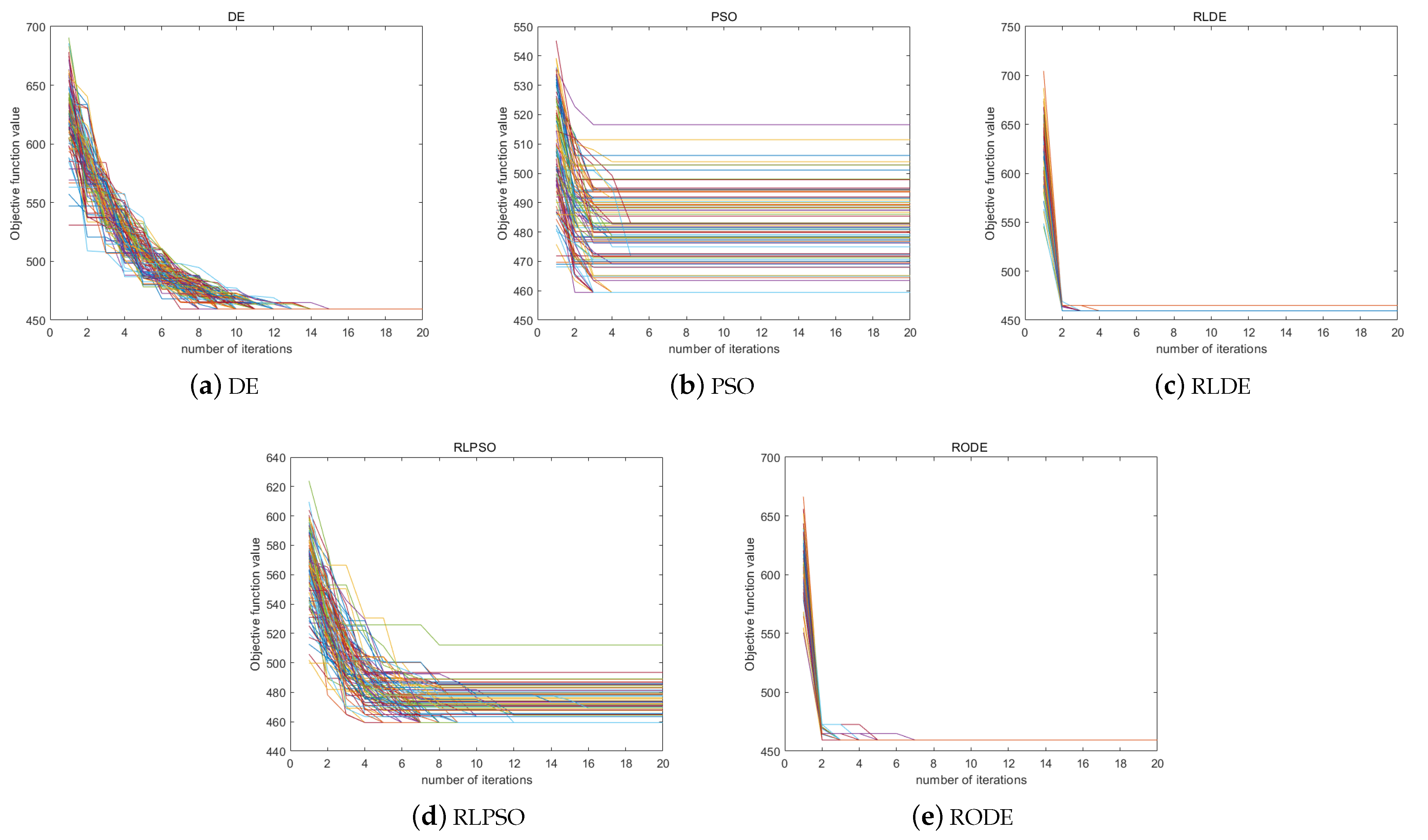
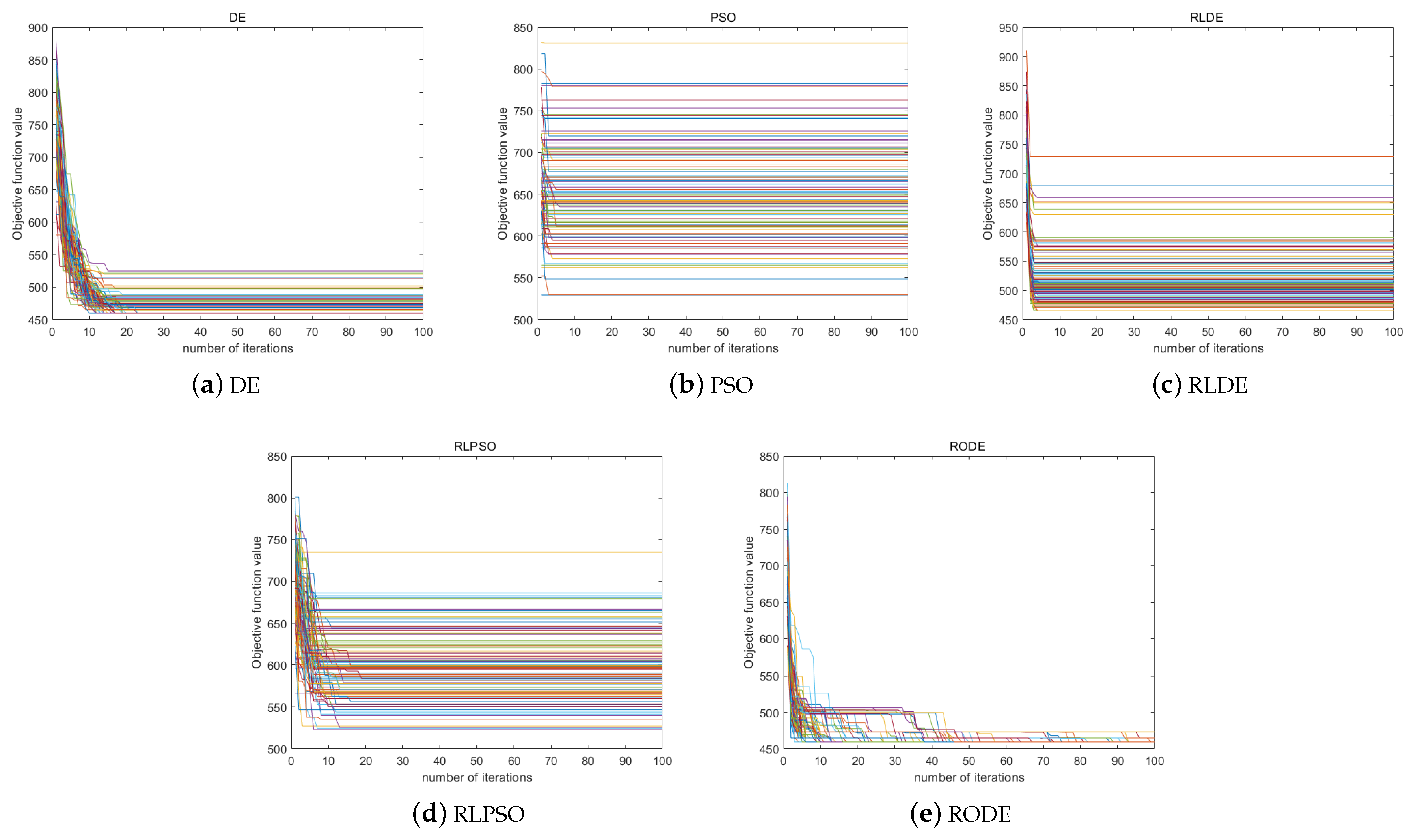
In order to further prove the good robustness of the RODE algorithm, we conducted the second type of experiments. This experiment is based on the initial population size of 200 and 10, and we let each algorithm run 100 times. Our main purpose is to observe the convergence speed and convergence accuracy of various algorithms under different initial population sizes.

The experimental results when the initial population size is 200 are shown in Figure 10. Among them, PSO falls into the local optimal solution 91 times, DE falls into the local optimal solution zero times, RLPSO falls into the local optimal solution 76 times, RLDE falls into the local optimal solution four times, and RODE falls into the local optimal solution zero times. Although neither DE nor the RODE algorithm has fallen into local optimization, it is obvious that RODE has converged near the optimal solution in the second generation, and its convergence speed is significantly faster than that of DE. At the same time, it can be seen that the convergence speed of the algorithm that introduced reinforcement learning has been significantly improved.

The experimental results when the initial population size is 10 are shown in Figure 11.

When the initial population size is 10, PSO falls into the local optimal solution 100 times, DE falls into the local optimal solution 75 times, RLPSO falls into the local optimal solution 99 times, and RLDE falls into the local optimal solution 99 times. There are 16 times the RODE becomes stuck in a local optimal solution. For this reason, we can see that when the initial population size is only 10, except for the RODE algorithm that introduces opposition-based learning, the convergence accuracy of the remaining algorithms is extremely poor. The comparison results of RODE and other algorithms are shown in the following

Table 6. The number of times each algorithm falls into the local optimal solution.

Algorithm	200	10
PSO	91	100
RLPSO	76	99
DE	0	75
RLDE	4	99
RODE	0	16

.

Through the comparison of two experiments, we can find that when the initial population size is large, the convergence accuracy of the algorithm is high, and the convergence speed of the algorithm incorporating reinforcement learning is significantly improved. When the population size is very small, the convergence performance of DE, PSO, RLPSO and RLDE algorithms becomes particularly poor, and it is difficult for them to jump out of the local optimal solution effectively under the condition of 100 iterations. However, RODE can still maintain a high convergence accuracy. This is because after the introduction of opposition-based learning, there is a high probability of jumping out of the local optimal solution in subsequent iterations, which is not available in other algorithms.

Therefore, the experimental results can prove that the RODE algorithm in this paper can largely resist the influence of the initial population, has strong robustness, and can quickly and accurately find the optimal strategy set. The disadvantage of this method is that it can only passively prevent attacks [39,40] in advance. If faced with frequent and changeable attack methods, the effect will be greatly discounted. For this reason, the main direction in the future is to study how to apply RODE to dynamic protection [41].

6.5. Discussion

As we all know, in view of the characteristics of industrial control security defense, the accuracy and speed of the selection strategy are particularly critical, which requires that the selected evolutionary algorithm not only solve the problem of convergence accuracy but also solve the problem of convergence speed, and consider the impact of population size. However, the previous evolutionary algorithms seem to focus on solving one of the problems, and they do not consider the effect of population size, because their tests are all carried out under the premise that the population size remains unchanged [7], while RODE considers the effect of population size. At the same time, reinforcement learning and opposition-based learning are also used to solve the problems of convergence speed and convergence accuracy, respectively. Furthermore, we verify the effectiveness of RODE at different population sizes through the above two sets of experiments.

Last but not least, in the second experiment, comparing RLDE and RODE in Figure 10, that is, when the population is 200, the performance of RODE and RLDE is almost the same, indicating that RODE has played a role in reinforcement learning. Comparing RLDE and RODE in Figure 11, that is, when the population is 10, the effect of RODE is much higher than that of RODE, because RODE has the effect of opposition-based learning at this time. So, we have reason to believe that RODE greatly improves the performance of the DE algorithm, and our method also provides a good idea for improving other evolutionary algorithms.

7. Conclusions

The scientific deployment of security strategies is the key to reducing the risk of ICS being attacked. In this paper, a differential evolution algorithm based on reinforcement learning and opposition-based learning is proposed to obtain the optimal security strategy by combining fitness functions. First, a Bayesian attack graph is used to model the potential attack paths of the industrial control system. Then, we calculate the attack benefit of each node and the cost of implementing the security strategy, and we build a fitness function based on the attack benefit and security cost. The fitness function can effectively evaluate the value of the selected solution. Finally, the RODE algorithm is used to select the security strategy scheme. The RODE algorithm is suitable for populations of various sizes. When the population size is large enough, the reinforcement learning in RODE can speed up the convergence rate; when the population size is relatively small, the opposition-based learning in RODE can increase the diversity of the population, thereby improving the ability to jump out of the local optimal solution and avoid the situation of premature convergence. A simplified water distribution system is used to validate the RODE algorithm. The experimental results show that the algorithm has better robustness than other algorithms of the same type, and it can find the optimal security strategy accurately and quickly. At present, our research is suitable for policy construction before the attack to minimize the loss of the attack, but it still has great shortcomings in dealing with the dynamic attack problem. To this end, in the future, we work on combining the RODE algorithm with policy selection in the face of dynamic attacks.

References

- Chen, T.M.; Abu-Nimeh, S. Lessons from Stuxnet. Computer 2011, 44, 91–93. Available online: https://0-ieeexplore-ieee-org.brum.beds.ac.uk/abstract/document/5742014 (accessed on 17 September 2022). [CrossRef]
- Case, D.U. Analysis of the cyber attack on the Ukrainian power grid. Electr. Inf. Shar. Anal. Cent. (E-ISAC) 2016, 388, 1–29. Available online: https://africautc.org/wp-content/uploads/2018/05/E-ISAC_SANS_Ukraine_DUC_5.pdf (accessed on 17 September 2022).
- Nespoli, P.; Papamartzivanos, D.; Mármol, F.G.; Kambourakis, G. Optimal countermeasures selection against cyber attacks: A comprehensive survey on reaction frameworks. IEEE Commun. Surv. Tutorials 2017, 20, 1361–1396. Available online: https://0-ieeexplore-ieee-org.brum.beds.ac.uk/abstract/document/8169023 (accessed on 17 September 2022). [CrossRef]
- Zhao, D.; Wang, L.; Wang, Z.; Xiao, G. Virus propagation and patch distribution in multiplex networks: Modeling, analysis, and optimal allocation. IEEE Trans. Inf. Forensics Secur. 2018, 14, 1755–1767. Available online: https://0-ieeexplore-ieee-org.brum.beds.ac.uk/abstract/document/8565928 (accessed on 17 September 2022). [CrossRef]
- Lee, C.; Han, S.M.; Chae, Y.H.; Seong, P.H. Development of a cyberattack response planning method for nuclear power plants by using the Markov decision process model. Ann. Nucl. Energy 2022, 166, 108725. Available online: https://0-www-sciencedirect-com.brum.beds.ac.uk/science/article/pii/S0306454921006010 (accessed on 17 September 2022). [CrossRef]
- Dewri, R.; Ray, I.; Poolsappasit, N.; Whitley, D. Optimal security hardening on attack tree models of networks: A cost-benefit analysis. Int. J. Inf. Secur. 2012, 11, 167–188. Available online: https://linkspringer.53yu.com/article/10.1007/s10207-012-0160-y (accessed on 17 September 2022). [CrossRef]
- Poolsappasit, N.; Dewri, R.; Ray, I. Dynamic security risk management using bayesian attack graphs. IEEE Trans. Dependable Secur. Comput. 2011, 9, 61–74. Available online: https://0-ieeexplore-ieee-org.brum.beds.ac.uk/abstract/document/5936075 (accessed on 17 September 2022). [CrossRef]
- Yang, X.S. A new metaheuristic bat-inspired algorithm. In Nature Inspired Cooperative Strategies for Optimization (NICSO 2010); Springer: Berlin/Heidelberg, Germany, 2010; pp. 65–74. Available online: https://linkspringer.53yu.com/chapter/10.1007/978-3-642-12538-6_6 (accessed on 17 September 2022).
- Meng, Z.; Yang, C. Two-stage differential evolution with novel parameter control. Inf. Sci. 2022, 596, 321–342. Available online: https://0-www-sciencedirect-com.brum.beds.ac.uk/science/article/pii/S0020025522002547 (accessed on 17 September 2022). [CrossRef]
- Dixit, A.; Mani, A.; Bansal, R. An adaptive mutation strategy for differential evolution algorithm based on particle swarm optimization. Evol. Intell. 2022, 15, 1571–1585. Available online: https://linkspringer.53yu.com/article/10.1007/s12065-021-00568-z (accessed on 17 September 2022). [CrossRef]
- Kaelbling, L.P.; Littman, M.L.; Moore, A.W. Reinforcement learning: A survey. J. Artif. Intell. Res. 1996, 4, 237–285. Available online: https://www.jair.org/index.php/jair/article/view/10166 (accessed on 17 September 2022). [CrossRef]
- Xu, Z.; Han, G.; Liu, L.; Martínez-García, M.; Wang, Z. Multi-energy scheduling of an industrial integrated energy system by reinforcement learning-based differential evolution. IEEE Trans. Green Commun. Netw. 2021, 5, 1077–1090. Available online: https://0-ieeexplore-ieee-org.brum.beds.ac.uk/abstract/document/9361643 (accessed on 17 September 2022). [CrossRef]
- Liao, Z.; Li, S. Solving Nonlinear Equations Systems with an Enhanced Reinforcement Learning Based Differential Evolution. Complex Syst. Model. Simul. 2022, 2, 78–95. Available online: https://0-ieeexplore-ieee-org.brum.beds.ac.uk/abstract/document/9770100 (accessed on 17 September 2022). [CrossRef]
- Tizhoosh, H.R. Opposition-based learning: A new scheme for machine intelligence. In Proceedings of the International Conference on Computational Intelligence for Modelling, Control and Automation and International Conference on Intelligent Agents, Web Technologies and Internet Commerce (CIMCA-IAWTIC’06, Vienna, Austria, 28–30 November 2005; Volume 1, pp. 695–701. Available online: https://0-ieeexplore-ieee-org.brum.beds.ac.uk/abstract/document/1631345 (accessed on 17 September 2022).
- Deng, W.; Ni, H.; Liu, Y.; Chen, H.; Zhao, H. An adaptive differential evolution algorithm based on belief space and generalized opposition-based learning for resource allocation. Appl. Soft Comput. 2022, 127, 109419. Available online: https://0-www-sciencedirect-com.brum.beds.ac.uk/science/article/pii/S1568494622005518 (accessed on 17 September 2022). [CrossRef]
- Abed-alguni, B.H.; Paul, D. Island-based Cuckoo Search with elite opposition-based learning and multiple mutation methods for solving optimization problems. Soft Comput. 2022, 26, 3293–3312. Available online: https://linkspringer.53yu.com/article/10.1007/s00500-021-06665-6 (accessed on 17 September 2022). [CrossRef]
- Tubishat, M.; Idris, N.; Shuib, L.; Abushariah, M.A.; Mirjalili, S. Improved Salp Swarm Algorithm based on opposition based learning and novel local search algorithm for feature selection. Expert Syst. Appl. 2020, 145, 113122. Available online: https://0-www-sciencedirect-com.brum.beds.ac.uk/science/article/abs/pii/S0957417419308395 (accessed on 17 September 2022). [CrossRef]
- Hussien, A.G.; Amin, M. A self-adaptive Harris Hawks optimization algorithm with opposition-based learning and chaotic local search strategy for global optimization and feature selection. Int. J. Mach. Learn. Cybern. 2022, 13, 309–336. Available online: https://linkspringer.53yu.com/article/10.1007/s13042-021-01326-4 (accessed on 17 September 2022). [CrossRef]
- Rahnamayan, S.; Tizhoosh, H.R.; Salama, M.M. Opposition-based differential evolution algorithms. In Proceedings of the 2006 IEEE International Conference on Evolutionary Computation, Vancouver, BC, Canada, 16–21 July 2006; pp. 2010–2017. Available online: https://0-ieeexplore-ieee-org.brum.beds.ac.uk/abstract/document/1688554 (accessed on 17 September 2022).
- Fister, I.; Fister, D. Reinforcement Learning-Based Differential Evolution for Global Optimization. In Differential Evolution: From Theory to Practice; Springer: Berlin/Heidelberg, Germany, 2022; pp. 43–75. Available online: https://linkspringer.53yu.com/chapter/10.1007/978-981-16-8082-3_3 (accessed on 17 September 2022).
- Hu, Z.; Gong, W.; Li, S. Reinforcement learning-based differential evolution for parameters extraction of photovoltaic models. Energy Rep. 2021, 7, 916–928. Available online: https://0-www-sciencedirect-com.brum.beds.ac.uk/science/article/pii/S2352484721000974 (accessed on 17 September 2022). [CrossRef]
- Huynh, T.N.; Do, D.T.; Lee, J. Q-Learning-based parameter control in differential evolution for structural optimization. Appl. Soft Comput. 2021, 107, 107464. Available online: https://0-www-sciencedirect-com.brum.beds.ac.uk/science/article/abs/pii/S1568494621003872 (accessed on 17 September 2022). [CrossRef]
- Roy, A.; Kim, D.S.; Trivedi, K.S. Scalable optimal countermeasure selection using implicit enumeration on attack countermeasure trees. In Proceedings of the IEEE/IFIP International Conference on Dependable Systems and Networks (DSN 2012), Boston, MA, USA, 25–28 June 2012; Available online: https://0-ieeexplore-ieee-org.brum.beds.ac.uk/abstract/document/6263940 (accessed on 17 September 2022).
- Wang, S.; Zhang, Z.; Kadobayashi, Y. Exploring attack graph for cost-benefit security hardening: A probabilistic approach. Comput. Secur. 2013, 32, 158–169. Available online: https://0-www-sciencedirect-com.brum.beds.ac.uk/science/article/pii/S0167404812001496 (accessed on 17 September 2022). [CrossRef]
- Khosravi-Farmad, M.; Ghaemi-Bafghi, A. Bayesian decision network-based security risk management framework. J. Netw. Syst. Manag. 2020, 28, 1794–1819. Available online: https://linkspringer.53yu.com/article/10.1007/s10922-020-09558-5 (accessed on 17 September 2022). [CrossRef]
- Gallon, L.; Bascou, J.J. Using CVSS in attack graphs. In Proceedings of the 2011 Sixth International Conference on Availability, Reliability and Security, Vienna, Austria, 22–26 August 2011; pp. 59–66. Available online: https://0-ieeexplore-ieee-org.brum.beds.ac.uk/abstract/document/6045939 (accessed on 17 September 2022).
- Qin, A.K.; Huang, V.L.; Suganthan, P.N. Differential evolution algorithm with strategy adaptation for global numerical optimization. IEEE Trans. Evol. Comput. 2008, 13, 398–417. Available online: https://0-ieeexplore-ieee-org.brum.beds.ac.uk/abstract/document/4632146 (accessed on 17 September 2022). [CrossRef]
- Hansen, N.; Ostermeier, A. Completely derandomized self-adaptation in evolution strategies. Evol. Comput. 2001, 9, 159–195. Available online: https://0-ieeexplore-ieee-org.brum.beds.ac.uk/abstract/document/6790628 (accessed on 17 September 2022). [CrossRef]
- Samma, H.; Lim, C.P.; Saleh, J.M. A new reinforcement learning-based memetic particle swarm optimizer. Appl. Soft Comput. 2016, 43, 276–297. Available online: https://0-www-sciencedirect-com.brum.beds.ac.uk/science/article/abs/pii/S1568494616000132 (accessed on 17 September 2022). [CrossRef]
- Watkins, C.J.; Dayan, P. Q-learning. Mach. Learn. 1992, 8, 279–292. Available online: https://linkspringer.53yu.com/article/10.1007/BF00992698 (accessed on 17 September 2022). [CrossRef]
- O’Donoghue, B.; Osband, I.; Munos, R.; Mnih, V. The uncertainty bellman equation and exploration. In Proceedings of the International Conference on Machine Learning, Stockholm, Sweden, 10–15 July 2018; pp. 3836–3845. Available online: http://proceedings.mlr.press/v80/o-donoghue18a/o-donoghue18a.pdf (accessed on 17 September 2022).
- Ming, H.; Wang, M.; Liang, X. An improved genetic algorithm using opposition-based learning for flexible job-shop scheduling problem. In Proceedings of the 2016 2nd International Conference on Cloud Computing and Internet of Things (CCIOT), Dalian, China, 22–23 October 2016; pp. 8–15. Available online: https://0-ieeexplore-ieee-org.brum.beds.ac.uk/abstract/document/7868294 (accessed on 17 September 2022).
- Agarwal, M.; Srivastava, G.M.S. Opposition-based learning inspired particle swarm optimization (OPSO) scheme for task scheduling problem in cloud computing. J. Ambient. Intell. Humaniz. Comput. 2021, 12, 9855–9875. Available online: https://linkspringer.53yu.com/article/10.1007/s12652-020-02730-4 (accessed on 17 September 2022). [CrossRef]
- Gämperle, R.; Müller, S.D.; Koumoutsakos, P. A parameter study for differential evolution. Adv. Intell. Syst. Fuzzy Syst. Evol. Comput. 2002, 10, 293–298. Available online: https://www.cse-lab.ethz.ch/wp-content/uploads/2008/04/gmk_wseas_2002.pdf (accessed on 17 September 2022).
- Si, T.; Miranda, P.B.; Bhattacharya, D. Novel enhanced Salp Swarm Algorithms using opposition-based learning schemes for global optimization problems. Expert Syst. Appl. 2022, 207, 117961. Available online: https://0-www-sciencedirect-com.brum.beds.ac.uk/science/article/abs/pii/S0957417422011940 (accessed on 17 September 2022). [CrossRef]
- Anderson, H. Introduction to Nessus. SecurityFocus Printable INFOCUS 2003. Available online: http://cryptomex.org/SlidesSeguRedes/TutNessus.pdf (accessed on 17 September 2022).
- Marini, F.; Walczak, B. Particle swarm optimization (PSO). A tutorial. Chemom. Intell. Lab. Syst. 2015, 149, 153–165. Available online: https://0-www-sciencedirect-com.brum.beds.ac.uk/science/article/abs/pii/S0169743915002117 (accessed on 17 September 2022). [CrossRef]
- Liu, Y.; Lu, H.; Cheng, S.; Shi, Y. An adaptive online parameter control algorithm for particle swarm optimization based on reinforcement learning. In Proceedings of the 2019 IEEE Congress on Evolutionary Computation (CEC), Wellington, New Zealand, 10–13 June 2019; pp. 815–822. Available online: https://0-ieeexplore-ieee-org.brum.beds.ac.uk/abstract/document/8790035 (accessed on 17 September 2022).
- Ades, S.; Herrera, D.A.; Lahey, T.; Thomas, A.A.; Jasra, S.; Barry, M.; Sprague, J.; Dittus, K.; Plante, T.B.; Kelly, J.; et al. Cancer care in the wake of a cyberattack: How to prepare and what to expect. JCO Oncol. Pract. 2022, 18, 23–34. Available online: https://0-www-sciencedirect-com.brum.beds.ac.uk/science/article/abs/pii/S1879850021002757 (accessed on 17 September 2022). [CrossRef]
- Teoh, A.A.; Ghani, N.B.A.; Ahmad, M.; Jhanjhi, N.; Alzain, M.A.; Masud, M. Organizational data breach: Building conscious care behavior in incident response. Comput. Syst. Sci. Eng. 2022, 40, 505–515. Available online: https://eprints.um.edu.my/33609/ (accessed on 17 September 2022). [CrossRef]
- Li, X.; Zhou, C.; Tian, Y.C.; Qin, Y. A dynamic decision-making approach for intrusion response in industrial control systems. IEEE Trans. Ind. Inform. 2018, 15, 2544–2554. Available online: https://0-ieeexplore-ieee-org.brum.beds.ac.uk/abstract/document/8443136 (accessed on 17 September 2022). [CrossRef] [Green Version]
Figure 1.
Optimal strategy selection framework for industrial control.
Figure 2.
Reinforcement learning description graph.