Article

Deep Neural Network Concept for a Blind Enhancement of Document-Images in the Presence of Multiple Distortions

by
Kabeh Mohsenzadegan
*,
Vahid Tavakkoli
and
Kyandoghere Kyamakya
Institute for Smart Systems Technologies, University Klagenfurt, 9020 Klagenfurt, Austria
*
Author to whom correspondence should be addressed.
Submission received: 24 July 2022 / Revised: 20 September 2022 / Accepted: 21 September 2022 / Published: 24 September 2022
(This article belongs to the Special Issue Image Enhancement and Restoration Based on Deep Learning Technology)

Abstract

:
In this paper, we propose a new convolutional neural network (CNN) architecture for improving document-image quality through decreasing the impact of distortions (i.e., blur, shadows, contrast issues, and noise) contained therein. Indeed, for many document-image processing systems such as OCR (optical character recognition) and document-image classification, the real-world image distortions can significantly degrade the performance of such systems in a way such that they become merely unusable. Therefore, a robust document-image enhancement model is required to preprocess the involved document images. The preprocessor system developed in this paper places “deblurring” and “noise removal and contrast enhancement” in two separate and sequential submodules. In the architecture of those two submodules, three new parts are introduced: (a) the patch-based approach, (b) preprocessing layer involving Gabor and Blur filters, and (c) the approach using residual blocks. Using these last-listed innovations results in a very promising performance when compared to the related works. Indeed, it is demonstrated that even extremely strongly degraded document images that were not previously recognizable by an OCR system can now become well-recognized with a 91.51% character recognition accuracy after the image enhancement preprocessing through our new CNN model.

1. Introduction

In the modern lifestyle, digital cameras are used extensively. However, document images captured from digital cameras are of a much lower or poorer quality than the ones obtained from traditional scanners concerning an optimal performance of subsequent document processing apps such as character recognition systems (OCR) [1,2,3,4] or document-image-based document classification systems [5,6] or visual speech recognition [7]. Indeed, document images acquired from digital cameras (possibly integrated into smartphones, which are very pervasive) are generally corrupted by various distortions such as noise, blur, shadow, geometric deformations, etc.
Therefore, one crucially needs some form of robust pre-enhancement before such significantly distorted document images can be given to either OCR or document classification systems. This ensures an acceptable confidence level for meaningful use in such mentioned applications. Figure 1 roughly illustrates both the input (s) (i.e., an image or some images) and the output of the blind enhancement module. It obtains a color image as the input and returns an enhanced image as the output. Examples of image enhancement preprocessing forms for such digital-camera-acquired document images are the following ones, separately or combined or integrated: deblurring, denoising, contrast improvement, adjusting the brightness, etc.
Image enhancement is widely used in atmospheric sciences [8], astrophotography [9], medical image processing [10], satellite image analysis, texture synthesis, remote sensing [11], digital photography, surveillance, and various video processing applications [12,13].
Image enhancement can be explained by using the following formula (see Equation (1)):
S = T ( D )
where S is the target image, D is the degraded input image, and T is a nonlinear function, transforming the degraded input image into its related “original” non-distorted image. For finding the function T , we can define a function Z in such a way that by minimizing it (i.e., by Z ), the function T will be converging to the required image enhancement function given in Equation (1). Thus, our target function Z is defined by using the following formula (see Equation (2)):
min Z = S e T ( D ) 2
where the S e is the expected or assumed original “clean “or non-distorted image.
On the other hand, it is well-known that the edges of or in character images are very important for a good performance on the OCR character recognition apps [14]. Therefore, we can add a so-called Sobel pre-filter to both sides of Equation (1). This results in the
S o b e l ( S ) = S o b e l ( T ( D ) )
By adding Equation (3) to our target function (see Equation (2)), we obtain the following new formula (see Equation (4)):
min Z = S e T ( D ) 2 + S o b e l ( S e ) S o b e l ( T ( D ) ) 2
where T is our target nonlinear function and S e is our expected original image. In Equation (4), we try to estimate the best-possible nonlinear function T by minimizing our target function Z described in Equation (4). This (i.e., Equation (4)) would be our loss function (while designing and training an appropriate deep convolutional neural network), which is used for estimating the nonlinear function T .
For estimating the function T , two different approaches exist, traditional methods and deep neural network concepts. Regarding the traditional methods, they essentially solve the problem via analytical and heuristic schemes [15,16]. In the second approach, such as the method proposed in this paper, convolutional neural network (CNN) models are used. CNN is a type of deep neural network which mainly uses, amongst others, convolution operations in its many layers. Deep neural networks (DNN) are essentially multi-layer artificial neural networks (ANN) [17] which are composed of four main parts or, better, functional bricks. These parts are convolution layers or filters, subsampling layers or filters, activation functions or layers, and “fully connected” neural network layers or blocks. Deep neural networks are, in essence, well-suited for performing a series of complex processing operations, e.g., estimating inverse filter(s), classification, denoising, contrast enhancement, etc. Previous studies have indeed proven that these types of networks can be used for denoising [18,19], contrast enhancement [20], and deblurring [21,22]. Thus, they have enough potential to reliably perform various image processing tasks.
The model we design in this paper involves CNN bricks, the concept of patches [23,24], the preprocessing Gabor and Blur filters [25,26,27], and finally the replacement of the repetitive hidden layers with residual blocks to increase convergence and the depth of network without adding complexity to it [28].
Section 2 briefly explains and discusses some related works regarding deblurring, denoising, contrast enhancement, and local light adjustment. Our novel CNN model is then described in Section 3. In Section 4, our model is then tested and compared or benchmarked with other selected relevant models while using or involving the same test dataset. In Section 5, concluding remarks are formulated, whereby the quintessence of the results obtained is briefly explained.

2. Related Works

The related works discussed in this section concern three different issues or distortions, which are all relevant and thus considered separately. These three different issues are: denoising, deblurring, and contrast or brightness enhancement. Although a given document image can be contaminated by a mixture of those distortions, they are addressed separately (i.e., in two functional modules) by our novel method.

2.1. Deblurring

Image blur is a significant distortion of document images. For example, images captured with moving or vibrating cameras may cause “motion blur”; the atmospheric turbulence can cause “Gaussian blur”, and “defocus blur” may be caused by the so-called lens aberrations [29].
The main problem of deblurring is the so-called deconvolution. Deblurring is an ill-posed problem. Thus, the final solution or clearing of the deconvolution should be optimized according to the specific type of image commonly used for deblurring. This type of optimization was introduced by Fergus et al. [30], and it was later extended by other authors who added and involved some ad hoc steps in providing an approximate solution [15,31,32,33]. For example, Levin et al. [34] added specific constraints to the problem to provide a correct solution to the so-called PSF (point spread function) problems. Therefore, using ad hoc steps and understanding well the precise nature of images at stake is crucial for finding appropriate solutions to the deconvolution problem.
Recently, CNN is used extensively in blind blur enhancement of images [35], and also most state-of-the-art methods are based on CNN [36]. The flexibility and power of CNN provides the possibility to improve the blur of an image blindly, especially in edges (Super Resolution). The CNN is also used in different forms such as hierarchical [37] and pyramid networks [38] to deblur the images. For example, one of the approaches involves Generative Adversarial Networks (GAN) in many related applications, such as super-resolution, blind denoising, and deblurring [39]. Xu et al. [40] have proposed such models to deblur text images.
Most of these related studies show some image quality improvement, but they are mainly capable of deblurring images with only a low magnitude of blur and mostly for the types Gaussian blur or mean blur. Therefore, a new model which can be used for other types of blurs such as motion blur is needed. Beyond that, in many cases, besides blur, other distortions may be present simultaneously.

2.2. Denoising

Various types of noises such as salt and pepper noise, Gaussian noise, Poisson noise, speckle noise, and many other fundamental noise types can contaminate document images and deteriorate the respective image quality [41].
Due to the ill-posed conditions of denoising, it is very important to know the original image’s statistical distribution. For example, some models have been introduced to emphasize the local area of pixel-like and total variation (TV) regularization [42]. Although those methods remove some noise from images, they also remove, unfortunately, some other good or important or needed details from images [43,44,45].
Recently, a patch-based approach is showing to be an up-and-coming solution to denoise images [46]. In most denoising schemes, the corrupted input image is decomposed by the denoiser into a set of patches, which will then be denoised separately, and later, those parts (i.e., denoised patches) are merged to create the final denoised image. One example of such a scheme is the so-called sparse coding method, which is trying to map each patch into a sparse coefficient matrix, in which most of the elements are zero or near to zero (sparse) [47,48].
A further scheme, a group method, works significantly better than the last described method, as most involved patches are Gaussian mixture models and have a multivariant correlation. Natural images are considered non-Gaussian, but they have one problem: they usually need more resources to be executed [46,49].
The idea of a patch-based solution comes from the fact they are inside (i.e., parts of a bigger) one image. We can find patches at different locations within the image, which can have similarities, and these similarities can be used by the denoiser to better reconstruct the original clean images. These similar patches are referred to in what is called non-local self-similarity (NSS). This method was first used in non-local mean denoising [50] and later, because of its precision and effectiveness, extended by different studies [46,49,51,52,53,54,55,56].
Denoising by using a convolutional neural network (CNN) was introduced by Jain et al. [57]. They argued that their algorithm or scheme achieved better results than traditional denoising methods such as total variation, wavelet approach, and other analytical techniques. Later, this CNN-based model was enhanced by introducing therein linear rectifier function(s) [58] and batch normalization [59].
Most of the above methods work well for white noise, but they hardly remove other kinds of noise such as salt noise, pepper noise, or speckle noise [53,60]. In addition, some of them introduce new distorting artifacts to the images (during the denoising process), which would need to be corrected or removed.

2.3. Contrast Enhancement and Local Light Adjustment

Most research defines contrast enhancement as adjusting the dynamic range of pixel intensity distribution for good contrast enhancement in images facing low contrast concerns. Contrast deterioration is mainly due to some external factors such as background light and environment.
Low-contrast images may reduce the visibility for digital users [61]. Most techniques for contrast enhancement are histogram-based or Retinex-based schemes [62]. In the histogram-based method, the main idea is that contrast-related pixel values globally or locally should have a Gaussian distribution. Therefore, these histogram-based techniques try to correct the pixel values’ distribution globally or locally according to a related window size definition [63]. Due to their simple functionality, they are easy to implement.
On the other hand, this histogram-based scheme in special situations hardly produces outstanding image quality, especially due to the complexity of image scenes and information loss in either low-contrast or high-contrast images. Further, they also eventually change the brightness of the processed image [64,65,66]. Therefore, several new related works have introduced new boundary conditions in the form of different regularization strategies.
For example, one can name the so-called Retinex-based method introduced by Land [67]. It is based on human color perception. The main concept of Retinex is based on composing illumination and reflections. The Single-Scale Retinex (SSR) is the implementation of center or surround Retinex. It provides reflectance as a result of the algorithm-like difference-of-Gaussian function. The Multi-Scale Retinex is similar to the previous one, but it contains a weighted sum of different SSR. Due to mapping color in an extra dimension, typically, after executing this algorithm, a color correction is required [62]. Both methods have also been implemented via convolutional neural networks, but the Retinex-based scheme has resulted in very low-contrast images [62].
Overall, a review of all related works shows a lack of good models that can significantly enhance document images containing certain distortion types (e.g., shadows, spotlights, etc.), and further, document images containing several distortion types simultaneously. Therefore, such a robust model that can face harshly distorted document images is very needed.

3. Our Novel Deep Neural Method for Blind Enhancement

The basic problem formulation is graphically presented in Figure 1, which essentially underscores the CNN deep neural model’s goal to be developed. However, for reaching the goal, it has been shown in the relevant literature that one single deep neural network cannot solve the complex problem at hand. Instead, a much more complex and modular deep neural architecture is needed. Indeed, the primary distorting artifacts that can be found in document images can be categorized into the following categories (see Figure 2):
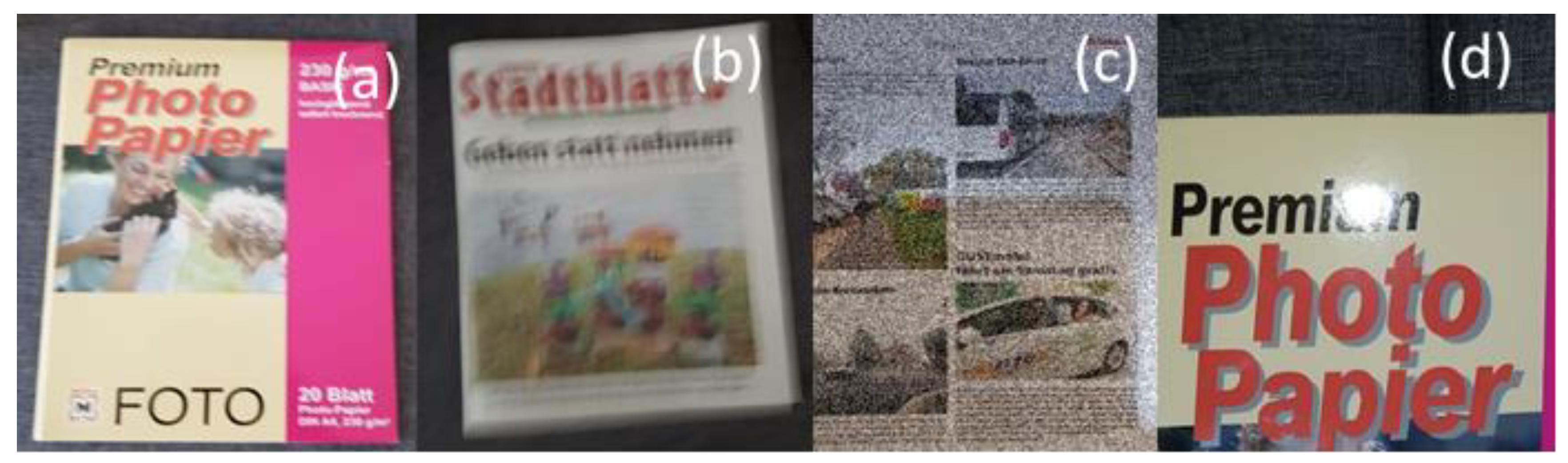
  • Blur problem(s), e.g., focus blur, Gaussian blur, motions blur, etc.;
  • Noise problem(s), e.g., salt noise or pepper noise, depending on image sensor sensitivity;
  • Contrast problem(s), e.g., shadows, spotlight, and contrast deficits.
For solving (removing) the mentioned distortions from a given document image, our overall model (see Figure 3) is designed with two sequential modules: (a) a document-image blur enhancement module, and (b) a document-image noise and contrast enhancement module.
The blur enhancement module is responsible for removing blur artifacts of the image. It has two types: motion blur and focus blur. The second module is responsible for eliminating or removing noise and contrast problems. The noise types can be salt and pepper noise and Gaussian noise. This module also improves contrast by fixing issues related to a spotlight, shadows, and overall image contrast enhancement.

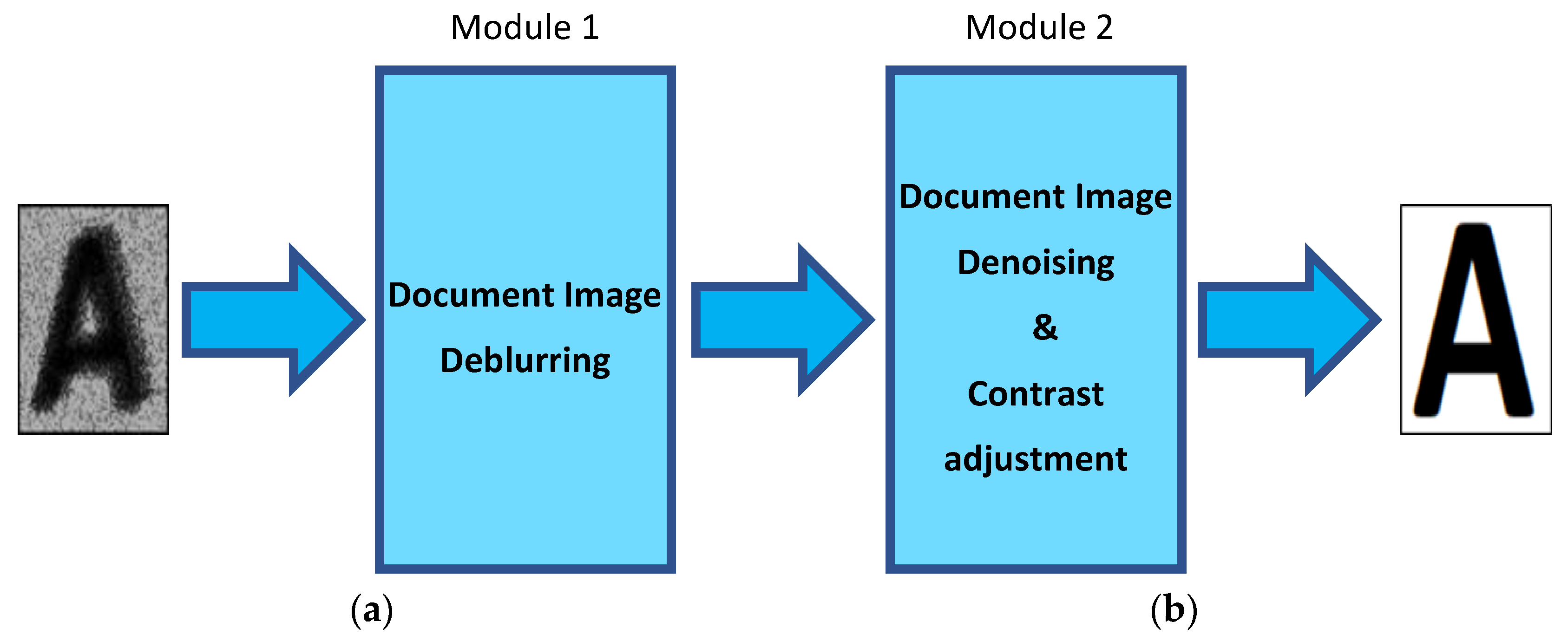
Document-Image Deblurring (Module 1, see Figure 3) and Document-Image Joint Contrast and Noise Enhancement (Module 2, See Figure 3)

Figure 4 shows the structure of our overall CNN architecture for deblurring, as well as contrast and noise enhancement. As we can see from a comprehensive review of the relevant state of the art, the enhancement process is one of the most challenging tasks in image enhancement research. Thereby, it is always required to perform various additional processing steps before the CNN model can enhance images with an acceptable resulting or final image quality. Therefore, in this work, we introduce two different steps before providing the input document image to the core convolutional neural network model. The input image in our illustrative experiments has a size of 246 × 246 pixels.
First, we split the image into small patches, all with the size of 128 × 128 pixels. The patches have a little overlap for later enabling a better reconstruction of the original complete image. In sum, in our illustrative experimental example, we have 12 images (each one patch) used for the next step (i.e., four split image patches, each with its corresponding three RGB channels). In a second step, we involve a bank of preprocessing layers, in which we intentionally add blur effects, Gabor with different blur, and Gabor kernels.
This set of blurred images and Gabor images, along with the original patches, are taken as our basis for the CNN model’s input (see Section A of Figure 4). The main idea behind this complex preprocessing structure is the intention of pre-filtering non-appropriate data. Each filter that is applied removes some uninteresting/non-appropriate information/data. Consequently, this results in a smaller neural network structure, and the related model training requires less time as this technique shrinks the searching area [25,26,27,68,69]. Figure 5 illustrates the effective impact of different parameters of the Gabor filter on the original image. It is worth mentioning that the pre-filtering processors do not yet enhance the input image, they just place it in a new intermediate state which enables the consecutive processing by the CNN model to perform much better. This is confirmed by the good performance reached.
In the main model, the residual blocks are used instead of pure convolutional layers (Section B of Figure 4). The residual block is formed by the first convolution layer, which is aligning the number of layers for the last summing. The output of this layer is duplicated into main and shortcut tensors. The main tensors go forward into a set of convolutional layers and batch normalization and finally are added to the shortcut tensor. This helps to increase the convergence by encapsulating the complexity into the residual blocks.
Increasing the number of (parallel) preprocessing layers to more extensive convolution layers enables the deblurring images with a larger magnitude of blur. On the other hand, it requires more images (test samples) to train and fulfill the converging model requirement to decrease the goal function given in Equation (4).
All those (parallel preprocessing) layers are concatenated together to create our inputs for our deep neural network.
All convolutional layers used in Figure 4 use the Relu activation function. Indeed, the Relu activation function [70] knowingly displays an outstanding convergence rate when compared to other activation functions.

4. Model Training and Discussion of the Results Obtained

The model’s training strategy is the most challenging part, and we need to consider different types of problems such as blur, noise, and contrast in the complex training process. Both quality and quantity of the training samples help better adjust or determine the weights in the CNN models. Each submodule converges into the best parameter settings because of each submodule’s final respective defined task.
The three following modules are used for creating the basic datasets. These datasets are used for the extensive comprehensive training of our models (see Figure 4 and Figure 5):
(a)
Blur generator module: this module is responsible for adding blur artifacts to the standard dataset for both training and testing purposes. It contains three types of blurs. These three types are focus, motion, and blur based on the PSF library.
(b)
Noise generator module: this module is responsible for adding noise artifacts to the standard dataset. It contains three types of noise. These three types are Gaussian, salt and pepper, and speckle noise types.
(c)
Contrast generator module: this module is responsible for adding low contrast and brightness effects to the standard dataset. It contains two types of artifacts. The first one is the contrast effect, and the second one is the brightness effect.
Three different reference datasets are used to create the training, validation, and verification datasets. The first dataset library contains 60,000 images from Hradis et al. [71]. It consists of cropped images from different scientific papers without any artifacts. The size of cropped images is 246 × 246 pixels. The second dataset library is gathered by our own team. It contains 6000 documents images and scanned images of different official documents such as driving licenses and identity cards with large sizes of 4000 × 4000 pixels. Then, artificial artifacts using Table 1 parameters are added to those images. This third dataset is a real-world one and is not generated by an artificial generator of distortions. Each document image is acquired under different distorting conditions such as noise, low contrast, spotlight, or shadows, which represent harsh real conditions. Based on the acquisition conditions of those documents, they have different various distorting artifacts, almost randomly. However, overall, we sort them into five quality categories or groups depending on how much the OCR readability (here: Tesseract OCR) is negatively affected. The five different quality categories are: very bad (under 60% OCR accuracy without enhancement), bad (6070% OCR accuracy without enhancement), average (7080% OCR accuracy without enhancement), good (8090% OCR accuracy without enhancement), very good (90100% OCR accuracy without enhancement). Document types contained therein are driving license, identity card, etc. For training purposes, the images are cropped in portions of 246 × 246 pixels.
These images of first and second datasets are mixed, and they are used as the source of images for our different artifact generators.
Consider creating a dataset for the training of the noise module. Here, one is adding noise to the original clean document-image samples from the original dataset to the first and second datasets. Hereby, one is adding different kinds of noise randomly, individually, or in a mixed form. The noise parameters used are shown in Table 1.
Consider creating a dataset for the training of the contrast and brightness module. Here, we add random contrast and brightness to the clean document images’ first and second dataset and truncate the contrast module’s pixel, exceeding the image threshold. The contrast and brightness parameters are shown in Table 1.
Consider creating a dataset for the training of the blur module. The blur module is the most advanced one. It contains various forms of blur: Gaussian, median, motion, and focus. With this, one adds different kinds of blur randomly, individually, or in a mixed form. The blur parameters are shown in Table 1.
The resized images described above are artificially distorted by adding blur for the first model’s module (see Figure 3) or artificially adding both contrast issues and noise for the second model’s module (see Figure 3). A set of 150,000 images have been used for training. In addition, for both verification and testing, datasets consisting of 40,000 images each were used.
In the first and second module, the ADAM [72] optimizer is used to train the model end-to-end. For a faster learning, the batch size of 128 images is selected. The learning rate of ADAM starts at 5 × 10⁻³, decreases by a decay rate of 0.95 after 100 epochs to improve the loss value, and finally stops at 1 × 10⁻⁵. The network is trained until it reaches 1000 epochs.
Equation (4) is used as loss function for training the model.
All developed CNN models (see Figure 3, Figure 4 and Figure 5) were implemented on a PC with Windows 10 Pro, Intel Core i7 9700K as CPU, double Nvidia GeForce GTX 1080 TI with 8 GB RAM as GPU, and 64 GB RAM. On this platform, the overall training of the developed model takes approximately 8 h.
The performance results obtained for each of the two modules of Figure 3 are compared with, i.e., benchmarked against, the selected best state-of-the-art models in their categories. That comparison was conducted based on two different metrics. The first metric is the peak signal-to-noise ratio (PSNR), and the second one is testing the amount of OCR-related errors after reading document images by Tesseract OCR [73] version 5.0.0. This last-mentioned source uses the peak signal-to-noise ratio, which is calculated through the following formula (see Equation (5)):
PSNR = 10   log (   255 2 MSE )
where MSE is the mean square error obtained by comparing the original clean or target image (ground truth) and the output image obtained from the enhancement models. This equation expresses the following fact: the lower the MSE, the higher the PSNR. Therefore, by increasing the amount of image quality, the value of PSNR will increase. For a further “quantitative” assessment or testing, we process all output images by a well-known OCR system called Tesseract. Tesseract is a free, open-source OCR software. All the sample outputs (deblurred, denoised) images were tested for readability by the Tesseract OCR [73] version 5.0.0.
Regarding the evaluation metrics for testing with OCR, we used two metrics which are generally used for assessing text recognition performance: the character recognition accuracy (CRA) and the word recognition accuracy (WCA). The CRA is the percentage of the number of characters recognized correctly per total number of characters, and the WCA is the percentage of the number of words recognized correctly. The related studies show that the WCA metric is generally used to compare text recognition performance of various schemes [74,75], therefore we used this metric to show the performance of our model.
The effect of newly introduced components such as blur and Gabor filters are examined based on the reference model of Hradis et al. [71]. Each of the new filter arrays are being added/removed (e.g., Gabor, blur) from the base model to show the performance based on the absence/presence of the respective component (ablation study). The newly introduced component will stay if it can improve the model behavior.
The next two sub-sections (Section 4.1 and Section 4.2) comprehensively explain and discuss the performance results of the first module and those of the second module of Figure 3.

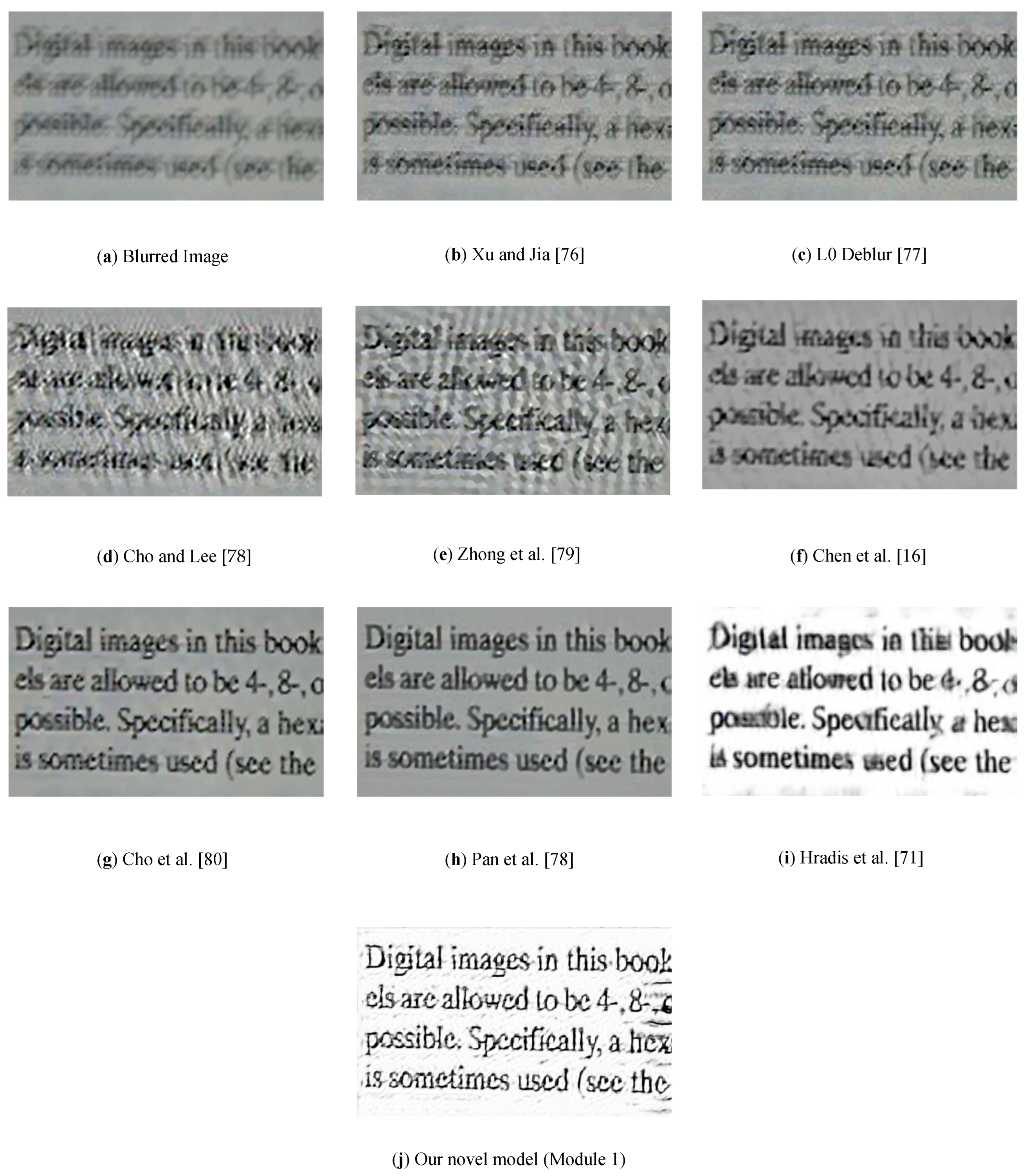
4.1. Performance Results of Module 1 (of Figure 3) for Document-Image Deblurring

In this sub-section, we compare the performance of Module 1 with a selection of well-known deblurring methods as presented in several recent papers from the relevant literature. Most of those methods from the literature are analytical, but only two of them are involving CNN.
In Figure 6, we present for illustration sample examples of deblurring results by Module 1. As we can see in these sample pictures, most of the output images have recognizable characters. However, their respective original images are not readable (by human eyes or by an OCR system).
In Figure 6, image (a) is the reference input blurred image, which has been, by the way, also used in several previous related studies. We can clearly see (through a qualitative visual inspection by human eyes) in Figure 6 that Module 1 produces a better-quality output image compared to those obtained by the other competing models from previous works (the two latest of them are CNN-based).
Table 2 shows the result of the ablation study. It is very clear that the base model improves while adding the new blur and Gabor filters.
For a further, this time “quantitative” testing, we now process all output images such as that in Figure 6 by a well-known OCR system called Tesseract (Figure 7 shows the output images obtained by Module 1; for the other models from the literature, the same input images are taken, and corresponding outputs are generated). Tesseract is a free, open-source OCR software. All the sample output (deblurred) images (shown in Figure 6) are tested for readability by the Tesseract OCR [73] version 5.0.0.
An overview of the evaluation results obtained in this comparative testing is shown in Table 3. Indeed, a good readability by the OCR system expresses the better quality of the enhanced image (obtained from the deblurring). Finally, the output images are also compared in terms of PSNR to show the “objective” quality of output images. The total number of images used for testing each model for producing the results of Table 2 was 1500 images. Those images were produced based on 100 images from the image dataset of Hradis et al. [71]; the blur types and parameters used are defined in Table 1.
The results presented in Table 3 above clearly show that most deblurring models result in a very large number of errors and can therefore not be used for reliably deblurring document images for a later reading by an OCR system. Although still weaker compared to that of Module 1, the only previous method with acceptable performance is the one by Pan et al. [78]. The concept of that model is, however, an analytical model, and reaches a performance of 92.48% character recognition accuracy (see Table 2). Amongst all results, our model (Module 1) shows a very good and the best performance ever, which is 94.55% character recognition accuracy (CRA).
Compared to the other solely CNN-based model (by Hradis et al. [78]) from the list of competing approaches in the benchmarking (see Table 3), our novel CNN model (Module 1) performs significantly better (Module 1: character accuracy rate of 94.55%, versus the other CNN model by Neji et al. [39] having a CRA of 69.55%).
Concerning PSNR, we also can see that our model is the best one, as it keeps color more in white noise and cleans the image much better.

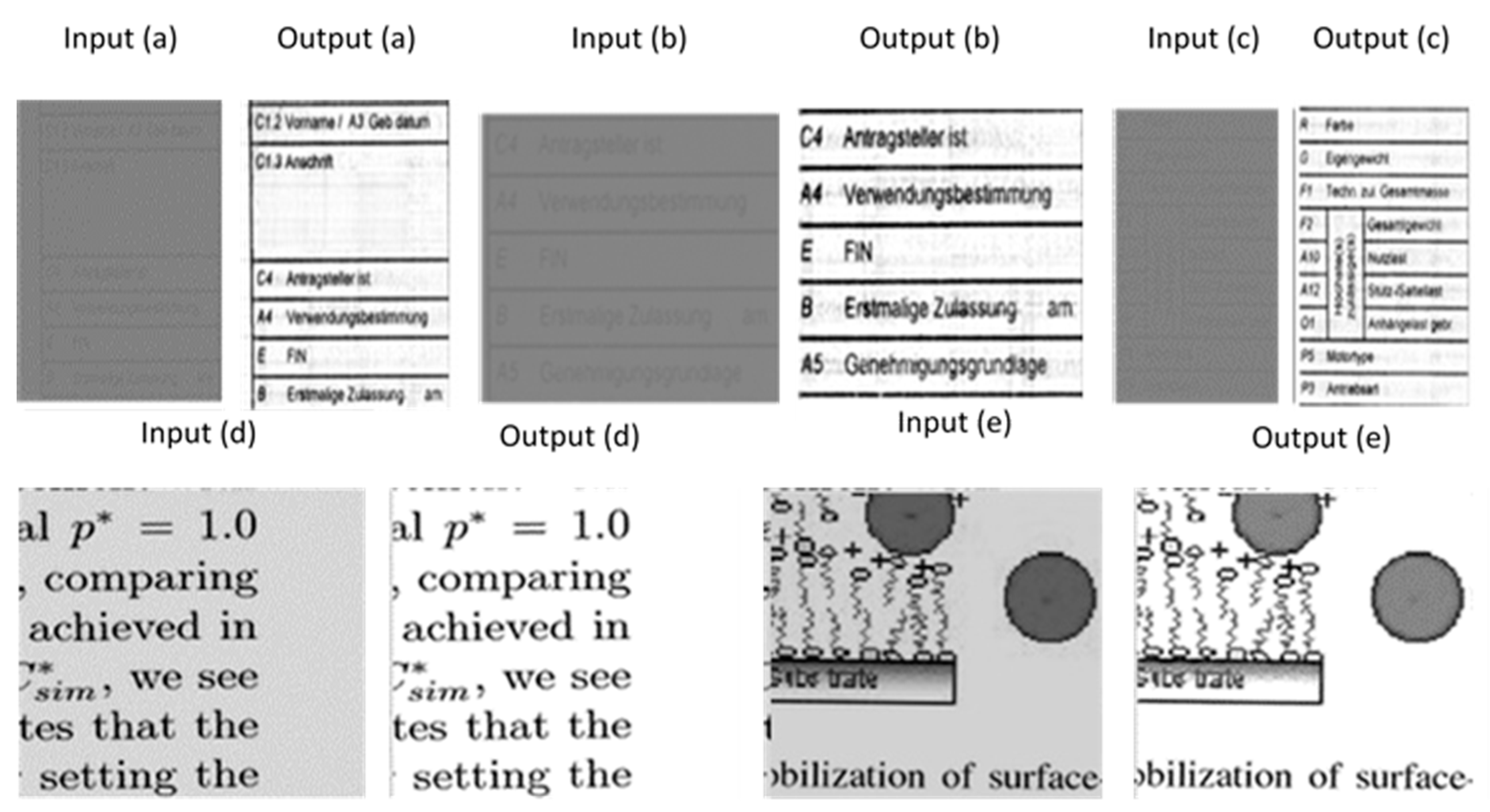
4.2. Performance Results with Regard to PSNR of Module 2 for Document-Image Noise Reduction and Contrast Improvement

In this sub-section, we provide and briefly discuss a set of illustrative performance results of Module 2. Figure 8 shows some selected inputs and outputs of the model of Module 2. As we explained previously, contrast and noise enhancement are blindly performed jointly in the second part of our global novel model, i.e., in Module 2 of Figure 3. Indeed, Figure 8 clearly shows that contrast and noise reduction are performed simultaneously.
For comprehensively measuring the performance of Module 2, we need an appropriate quality metric to better assess the efficiency of the “noise removal + contrast enhancement” module. For this purpose, we introduce and use a metric which was explained by Fu et al. [60]. This last-mentioned source uses the peak signal-to-noise ratio, which is calculated through the explained formula (see Equation (5)) .
Concerning noise, we compare the performance of Module 2 with some related models published in recent papers from the literature. Hereby, we consider the so-called salt noise. The models from the literature were trained mainly for salt noise, but our model is also trained and tested for Gaussian noise.
Figure 9 shows the performance of our model compared to state-of-the-art models for denoising images. The original image contains peppers. One part of the peppers is zoomed in to show the sharp part of the peppers. That image is used as the original image, and a 50% noise level is added to that image. One can see how each model tries to reduce the noise level, whereby our model outperforms the other models when considering the sharpness of the respective enhanced image.
Table 4 shows the PSNR performance of the different denoising models used by Fu et al. [60]. The images are the same as in the source Fu et al. [60] to make a comprehensive comparison possible. The number of test images were 11 images from the standard test images (“Pepper”, “Lena”, “Baboon”, “Bridge”, “Barbara”, “Fruit”, “Cameraman”, “House”, “Starfish”, “Monarch”, “Plane”) and 100 images from the Hradis et al. [78] test dataset. Some of the results of single images such as Lena and Pepper directly show the difference amongst the results obtained from the different involved models.
We can see (see Table 3) that our model provides the best PSNR results compared to the other models. For example, compared to the Fu et al. [60] model, our model shows a PSNR improvement ranging between 5% to 8%.

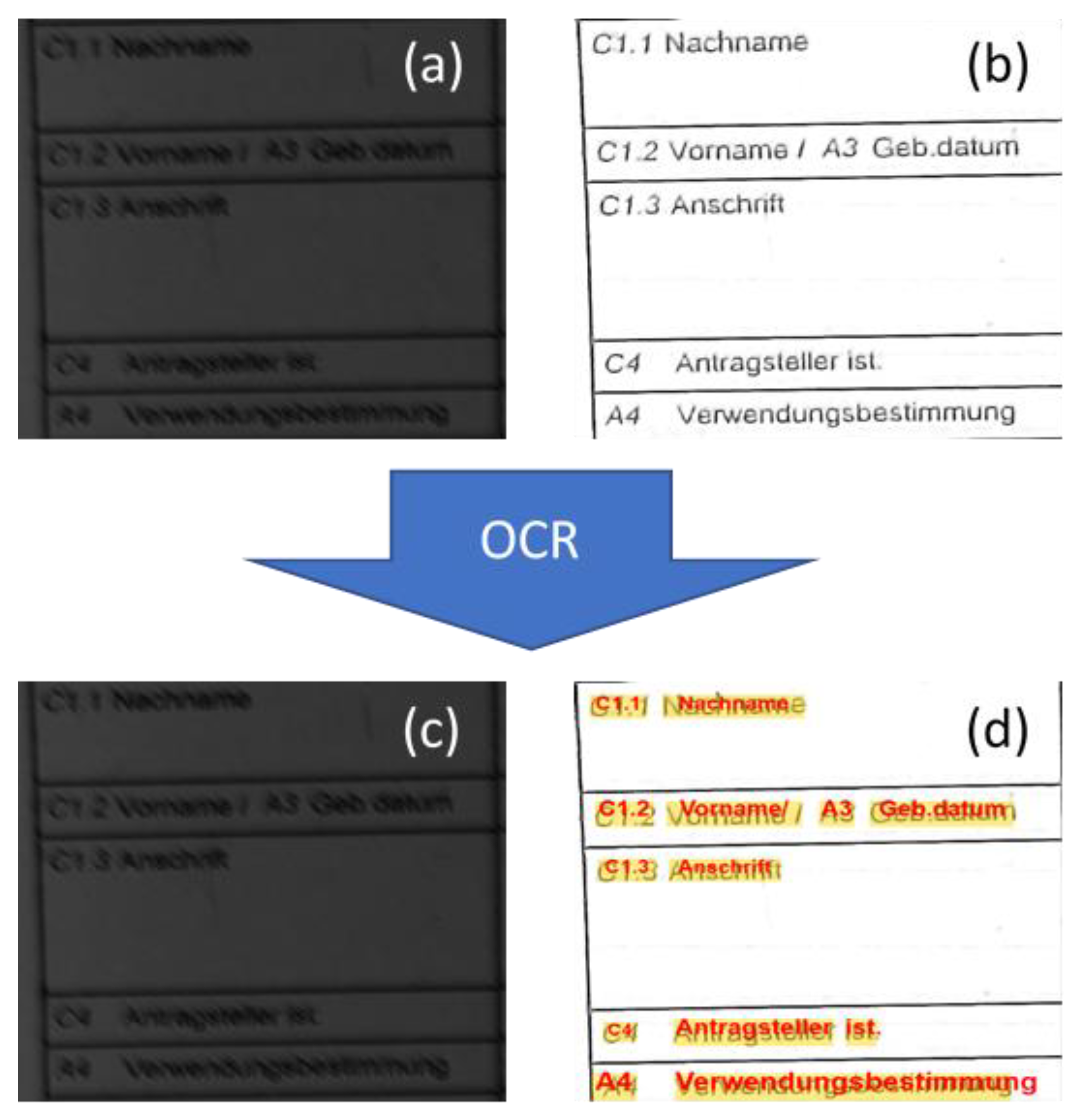
4.3. Performance Results with Respect to the OCR Performance of Module 2 for Document-Image Contrast and Brightness Enhancement

One of the sensitive problems while recognizing text through OCR is low contrast and brightness issues. An improvement of the text contrast makes the dark or highlighted parts more readable. For example, the input texts in Figure 10 are not recognizable by an OCR software, but after their contrast and brightness are adjusted, they can recognize text with 95% accuracy. Figure 10 shows that the second module is capable of significant contrast and brightness enhancement.

4.4. Performance Evaluation of Our Novel Global Model including “Module 1 + Module 2” (of Figure 3) for Blindly Enhancing Document Images Simultaneously Distorted by Blur + Noise + Contrast

After comparing comprehensively the performance of separated submodules in the previous sub-sections in the presence of different artifacts, we discuss in this section the overall performance of the global model (Module 1 + Module 2) compared to other competing related models in the presence of a mix of artifacts or distortions; this test context shall be considered as an extreme stress test of the performance of the best models available.
The dataset which is presented in this section consists of document images obtained by our team in harsh acquisition conditions (by cameras) (see Figure 11). This selection of 100 samples has been used for stress testing the different models. As one can see on this collection of images, different forms of distortions are present in the images, for example noise, contrast, and shadows; mostly, various distortions are simultaneously present in the images. (Note: since the images do partially contain some personal data, those related parts have been covered by a black rectangle for privacy reasons.)
The main reason for these harsh conditions is to provide strongly distorted images (i.e., contaminated by a mixture of distortions) in order to better stress test the robustness of the models involved in a comprehensive benchmarking (our novel model and a selection of the top best models from the relevant literature).
Figure 12 shows, for illustration, the performance of our global model in the presence of sample document images captured by a mobile phone camera. As one can see, the image quality is significantly enhanced so that the OCR system that could previously (on the non-enhanced input images) not detect even a single character can now (after enhancement) catch all the text information without any problem. Image (a) in Figure 12 is the document that has a mixture of distortions, namely motion blur, contrast, and noise problems. Image (b) in Figure 12 is an enhanced image through our novel global model. Image (c) in Figure 12 is the output of the OCR by using image (a), whereby none of the text in the image (a) is detected. The image (d) in Figure 12 is the output of the OCR by using the image (b) in Figure 12, whereby all the texts in this image are well caught/detected by the OCR without any significant error (Figure 12d).
Table 5 shows the performance of our novel global model compared to the other related best models. For stress testing different models in this benchmarking, we used our dataset of real-world document images (obtained under harsh conditions) that mobile phone cameras have captured. One can see (see Table 4) that our model is about 13 percent better than the state-of-the-art model for deblurring combined with a state-of-the-art model for denoising. This test/benchmarking demonstrates and underscores the superiority of our novel model compared to a combination of the state-of-the-art best models. On the other hand, taken alone, the models developed solely for deblurring are not good enough for real-world hard cases; one can see that there are too many recognition errors in Figure 12c.

5. Conclusions

In this paper, we developed a new deep neural model to reliably and memory-efficiently deblur, denoise, and enhance the contrast of document images so that they become more readable for OCR software systems. This accuracy is achieved by sequentially combining two different enhancement modules, the first for deblurring and the second for jointly denoising and contrast enhancement. Each of these two named modules were appropriately trained with an appropriate specialized training set for the respective specific sub-tasks. This task separation shows an outstanding performance.
Our Module 1 model performs excellently in the blur part and outperforms other deblurring methods by generating the most recognizable text image. In the noise and contrast enhancement part, Module 2, the developed model shows a superb denoising effect compared to the previous salt and pepper denoising methods. It outperforms the best of those related models in the range of 5% to 8%. Our contrast is not comparable, as text contrast enhancement has a different meaning than other contrast enhancement types.
After enhancement, our global model’s output images are significantly more readable by an OCR system. This enhanced readability is reached even in cases of very strongly blur-distorted document images; we could see an accuracy improving from 13.56% to about 91.51%. A core limitation of the concept developed in this paper is that it is valid and has been validated so far only for document images and not for other types of images. Document images are different and specific compared to other more general image types. Thus, the specific image enhancement endeavor in the context of this paper has the sole purpose of making document images more readable by OCR systems. This is a very specific context and specification, which is not the same for all other types of images. For example, if a distorted marriage photo needs to be enhanced, the enhancement target does not necessarily match the ones of a document image. Indeed, an enhanced document image may still contain some form of dirt, especially in the background. However, the readability through an OCR of the text contained therein was significantly improved.
Therefore, possible future works of interest may relate to developing a novel global neural model which shall be optimized to various types of images as needed in various application contexts (examples of contexts: smartphone cameras, scene analysis or a self-driving car, video streaming through a smartphone, etc.).

Author Contributions

Conceptualization, K.M., V.T. and K.K.; Methodology, K.K.; Software, K.M. and V.T.; Validation, K.M., V.T. and K.K.; Formal Analysis, K.M.; Investigation, K.M. and V.T.; Resources, K.M.; Data Curation, K.M.; Writing—Original Draft Preparation, K.M. and V.T.; Writing—Review and Editing, K.M., V.T. and K.K.; Visualization, K.M. and V.T.; Supervision, K.K.; Project Administration, K.K. All authors have read and agreed to the published version of the manuscript.

Funding

This paper’s results were obtained in the frame of a project funded by UNIQUARE GmbH, Austria (Project Title: Dokumenten-OCR-Analyse und Validierung).

Institutional Review Board Statement

Not applicable.

Informed Consent Statement

Not applicable.

Acknowledgments

We thank the UNIQUARE employees Ralf Pichler, Olaf Bouwmeester, and Robert Zupan for their precious contributions and support.

Conflicts of Interest

The authors declare no conflict of interest.

References

  1. Chung, Y.; Chi, S.; Bae, K.S.; Kim, K.; Jang, D.; Kim, K.; Choi, Y. Extraction of character areas from digital camera based color document images and OCR system. In Proceedings of the SPIE- Optical Information Systems III, San Diego, CA, USA, 31 July–4 August 2005. [Google Scholar]
  2. Sharma, P.; Sharma, S. Image processing based degraded camera captured document enhancement for improved OCR accuracy. In Proceedings of the 2016 6th International Conference—Cloud System and Big Data Engineering (Confluence), Noida, India, 14–15 January 2016. [Google Scholar]
  3. Visvanathan, T.C.; Bhattacharya, U. Enhancement of camera captured text images with specular reflection. In Proceedings of the 2013 4th National Conference on Computer Vision, Pattern Recognition, Image Processing and Graphics (NCVPRIPG), Jodhpur, India, 18–21 December 2013. [Google Scholar]
  4. Tian, D.; Hao, Y.; Ha, M.; Tian, X.; Ha, Y. Algorithm of contrast enhancement for visual document images with underexposure. In Proceedings of the SPIE— International Symposium on Photoelectronic Detection and Imaging, Beijing, China, 7 March 2008. [Google Scholar]
  5. Lu, D.; Weng, Q. A survey of image classification methods and techniques for improving classification performance. J. Remote Sens. 2007, 28, 823–870. [Google Scholar] [CrossRef]
  6. Fan, M.; Huang, R.; Feng, W.; Sun, J. Image blur classification and blur usefulness assessment. In Proceedings of the 2017 IEEE International Conference on Multimedia & Expo Workshops (ICMEW), Hong Kong, China, 10–14 July 2017. [Google Scholar]
  7. Chan, Z.-M.; Lau, C.-Y.; Thang, K.-F. Visual Speech Recognition of Lips Images Using Convolutional Neural Network in VGG-M Model. J. Inf. Hiding Multimed. Signal Process. 2020, 11, 116–125. [Google Scholar]
  8. Jaleel, S.; Bhavya, V.; Sree, N.A.; Sajitha, P. Edge Enhancement Using Haar MotherWavelets for Edge Detection in SAR Images. Int. J. Innov. Res. Sci. Eng. Technol. 2014, 3, 5. [Google Scholar]
  9. Lucas, J.; Calef, B.; Knox, K. Image Enhancement for Astronomical Scenes. Proc. SPIE 2013, 8856, 885603. [Google Scholar]
  10. Umamaheswari, J.; Radhamani, G. An Enhanced Approach for Medical Brain Image Enhancement. J. Comput. Sci. 2012, 8, 1329–1337. [Google Scholar]
  11. Jadhav, D.; Patil, P.M. An effective method for satellite image enhancement. In Proceedings of the International Conference on Computing, Communication & Automation, Noida, India, 15–16 May 2015. [Google Scholar]
  12. Rahman, S.; Rahman, M.M.; Hussain, K.; Khaled, S.M.; Shoyaib, M. Image Enhancement in Spatial Domain: A Comprehensive Study. In Proceedings of the 2014 17th International Conference on Computer and Information Technology (ICCIT), Dhaka, Bangladesh, 22–23 December 2014. [Google Scholar]
  13. Hou, J.; Zhao, Y.; Lin, C.; Bai, H.; Liu, M. Quality Enhancement of Compressed Video via CNNs. J. Inf. Hiding Multimed. Signal Process. 2017, 8, 200–207. [Google Scholar]
  14. Huang, R.; Shivakumara, P.; Uchida, S. Scene character detection by an edge-ray filter. In Proceedings of the 12th International Conference on Document Analysis and Recognition, Washington, DC, USA, 25–28 August 2013. [Google Scholar]
  15. Almeida, M.; Almeida, L. Blind and Semi-Blind Deblurring of Natural Images. IEEE Trans. Image Process. 2010, 19, 36–52. [Google Scholar] [CrossRef] [PubMed]
  16. Chen, X.; He, X.; Yang, J.; Wu, Q. An effective document image deblurring algorithm. In Proceedings of the IEEE Computer Society Conference on Computer Vision and Pattern Recognition, San Juan, PR, USA, 17–19 June 2011. [Google Scholar]
  17. Kuang, X.; Sui, X.; Liu, Y.; Chen, Q.; Gu, G. Single infrared image enhancement using a deep convolutional neural network. Neurocomputing 2019, 332, 119–128. [Google Scholar] [CrossRef]
  18. Lefkimmiatis, S. Non-local Color Image Denoising with Convolutional Neural Networks. arXiv 2017, arXiv:1611.06757. [Google Scholar]
  19. Cruz, C.; Foi, A.; Katkovnik, V.; Egiazarian, K. Nonlocality-Reinforced Convolutional Neural Networks for Image Denoising. IEEE Signal Process. Lett. 2018, 25, 1216–1220. [Google Scholar] [CrossRef]
  20. Sun, J.; Kim, S.W.; Lee, S.W.; Ko, S. A novel contrast enhancement forensics based on convolutional neural networks. Signal Process.-Image Commun. 2018, 63, 149–160. [Google Scholar] [CrossRef]
  21. Niu, W.; Zhang, K.; Luo, W.; Zhong, Y. Blind motion deblurring super-resolution: When dynamic spatio-temporal learning meets static image understanding. IEEE Trans. Image Process. 2021, 30, 7101–7111. [Google Scholar] [CrossRef] [PubMed]
  22. Nah, S.; Kim, T.H.; Lee, K.M. Deep Multi-scale Convolutional Neural Network for Dynamic Scene Deblurring. arXiv 2017, arXiv:1612.02177. [Google Scholar]
  23. Po, L.-M.; Liu, M.; Yuen, W.Y.F.; Li, Y.; Xu, X.; Zhou, C.; Wong, P.H.W.; Lau, K.W.; Luk, H.-T. A Novel Patch Variance Biased Convolutional Neural Network for No-Reference Image Quality Assessment. IEEE Trans. Circuits Syst. Video Technol. 2019, 29, 1223–1229. [Google Scholar] [CrossRef]
  24. Zhang, Y.; Lin, H.; Li, Y.; Ma, H. A Patch Based Denoising Method Using Deep Convolutional Neural Network for Seismic Image. IEEE Access 2019, 7, 156883–156894. [Google Scholar] [CrossRef]
  25. Yao, H.; Chuyi, L.; Dan, H.; Weiyu, Y. Gabor Feature Based Convolutional Neural Network for Object Recognition in Natural Scene. In Proceedings of the 2016 3rd International Conference on Information Science and Control Engineering (ICISCE), Bejing, China, 8–10 July 2016. [Google Scholar]
  26. Hosseini, S.; Lee, S.; Kwon, H.; Koo, H.; Cho, N. Age and gender classification using wide convolutional neural network and Gabor filter. In Proceedings of the 2018 International Workshop on Advanced Image Technology (IWAIT), Chiang Mai, Thailand, 7–9 January 2018. [Google Scholar]
  27. Nguyen, V.; Lim, K.; Le, M.; Bui, N. Combination of Gabor Filter and Convolutional Neural Network for Suspicious Mass Classification. In Proceedings of the 2018 22nd International Computer Science and Engineering Conference (ICSEC), Chiang Mai, Thailand, 21–24 November 2018. [Google Scholar]
  28. He, K.; Zhang, X.; Ren, S.; Sun, J. Deep Residual Learning for Image Recognition. arXiv 2015, arXiv:1512.03385. [Google Scholar]
  29. Yiren, Z.; Sibo, S.; Cheung, N. On Classification of Distorted Images with Deep Convolutional Neural. In Proceedings of the International Conference on Acoustics, Speech and Signal Processing, New Orlean, LA, USA, 5–9 March 2017. [Google Scholar]
  30. Fergus, R.; Singh, B.; Hertzmann, A.; Roweis, S.T.; Freeman, W.T. Removing camera shake from a single photograph. ACM Trans. Graph. 2006, 25, 787–794. [Google Scholar] [CrossRef]
  31. Bunyak, Y.; Sofina, O.; Kvetnyy, R. Blind PSF estimation and methods of deconvolution optimization. arXiv 2012, arXiv:1206.3594. [Google Scholar]
  32. Krishnan, T.T.; Fergus, R. Blind deconvolution using a normalized sparsity measure. In Proceedings of the IEEE Computer Society Conference on Computer Vision and Pattern Recognition, Washington, DC, USA, 20–25 June 2011. [Google Scholar]
  33. Sun, S.; Zhao, H.; Li, B.; Hao, M.; Lv, J. Kernel estimation for robust motion deblurring of noisy and blurry images. J. Electron. Imaging 2016, 25, 033019. [Google Scholar] [CrossRef]
  34. Levin, A.; Weiss, Y.; Durand, F.; Freeman, W.T. Understanding Blind Deconvolution Algorithms. IEEE Trans. Pattern Anal. Mach. Intell. 2011, 33, 2354–2367. [Google Scholar] [CrossRef]
  35. Albluwi, V.K.; Dahyot, R. Image Deblurring and Super-Resolution Using Deep Convolutional Neural Networks. In Proceedings of the IEEE International Workshop on Machine Learning for Signal Processing, AALBORG, Aalborg, Denmark, 17–20 September 2018. [Google Scholar]
  36. Liu, Z.S.; Siu, W.C.; Chan, Y.L. Reference Based Face Super-Resolution. IEEE Access 2019, 7, 129112–129126. [Google Scholar] [CrossRef]
  37. Liu, B.; Ait-Boudaoud, D. Effective image super resolution via hierarchical convolutional neural network. Neurocomputing 2020, 374, 109–116. [Google Scholar] [CrossRef]
  38. Lai, W.S.; Huang, J.B.; Ahuja, N.; Yang, M.H. Fast and Accurate Image Super-Resolution with Deep Laplacian Pyramid Networks. IEEE Trans. Pattern Anal. Mach. Intell. 2019, 41, 2599–2613. [Google Scholar] [CrossRef] [PubMed]
  39. Neji, H.; Halima, M.; Hamdani, T.; Nogueras-Iso, J.; Alimi, A. Blur2Sharp: A GAN-Based Model for Document Image Deblurring. Int. J. Comput. Intell. Syst. 2021, 14, 1315–1321. [Google Scholar] [CrossRef]
  40. Xu, X.; Sun, D.; Pan, J.; Zhang, Y.; Pfister, H.; Yang, M.H. Learning to super-resolve blurry face and text images. In Proceedings of the 2017 IEEE International Conference on Computer Vision (ICCV), Venice, Italy, 22–29 October 2017. [Google Scholar]
  41. Khaw, H.Y.; Soon, F.C.; Chuah1, J.H.; Chow, C.-O. Image noise types recognition using. IET Image Process. 2017, 11, 1238–1245. [Google Scholar] [CrossRef]
  42. Liu, K.; Tan, J.; Su, B. An adaptive image denoising model based on tikhonov and TV regularizations. Adv. Multimed. 2014, 2014, 8. [Google Scholar] [CrossRef]
  43. Shahdoosti, H.Z. Edge-preserving image denoising using a deep convolutional neural network. Signal Process. 2019, 159, 20–32. [Google Scholar] [CrossRef]
  44. Chen, J.L.F. Denoising convolutional neural network with mask for salt and pepper noise. IET Image Process. 2019, 13, 2604–2613. [Google Scholar] [CrossRef]
  45. Thakur, R.S.; Yadav, R.N.; Gupta, L. State-of-art analysis of image denoising methods using convolutional neural networks. IET Image Process. 2019, 13, 2367–2380. [Google Scholar]
  46. Alkinani, M.H.; El-Sakka, M.R. Patch-based models and algorithms for image denoising: A comparative review between patch-based images denoising methods for additive noise reduction. Eurasip J. Image Video Process. 2017, 2017, 58. [Google Scholar] [CrossRef]
  47. Nejati, M.; Samavi, S.; Derksen, H.; Najarian, K. Denoising by low-rank and sparse representations. J. Vis. Commun. Image Represent. 2016, 36, 28–39. [Google Scholar] [CrossRef]
  48. Zha, Z.; Liu, X.; Zhou, Z.; Huang, X.; Shi, J.; Shang, Z.; Tang, L.; Bai, Y.; Wang, Q.; Zhang, X. Image denoising via group sparsity residual constraint. In Proceedings of the IEEE International Conference on Acoustics, Speech and Signal Processing, New Orleans, LA, USA, 5–9 March 2017. [Google Scholar]
  49. Hu, H.; Froment, J.; Liu, Q. A note on patch-based low-rank minimization for fast image denoising. J. Vis. Commun. Image Represent. 2018, 50, 100–110. [Google Scholar] [CrossRef]
  50. Buades, B.C.; Morel, J.M. Non-Local Means Denoising. Image Process. On Line 2011, 1, 208–212. [Google Scholar] [CrossRef]
  51. Chatterjee, P.; Milanfar, P. Patch-Based Near-Optimal Image Denoising. IEEE Trans. Image Process. 2012, 21, 1635–1649. [Google Scholar] [CrossRef]
  52. Zhou, T.; Li, C.; Zeng, X.; Zhao, Y. Sparse representation with enhanced nonlocal self-similarity for image denoising. Mach. Vis. Appl. 2021, 32, 1–11. [Google Scholar] [CrossRef]
  53. Kishan, H.; Seelamantula, C.S. Patch-based and multiresolution optimum bilateral filters for denoising images corrupted by Gaussian noise. J. Electron. Imaging 2015, 24, 053021. [Google Scholar] [CrossRef]
  54. Fu, B.; Zhao, X.-Y.; Li, Y.; Wang, X. Patch-based contour prior image denoising for salt and pepper noise. Multimed. Tools Appl. 2019, 78, 30865–30875. [Google Scholar] [CrossRef]
  55. Lu, S. Good Similar Patches for Image Denoising. arXiv 2019, arXiv:1901.06046. [Google Scholar]
  56. Jain, P.; Tyagi, V. LAPB: Locally adaptive patch-based wavelet domain edge-preserving image denoising. Inf. Sci. 2015, 294, 164–181. [Google Scholar] [CrossRef]
  57. Jain, V.; Seung, H.S. Natural Image Denoising with Convolutional Networks. In Proceedings of the Advances in Neural Information Processing Systems 21 (NIPS 2008), Vancouver, BC, Canada, 8–11 December 2008. [Google Scholar]
  58. Krizhevsky, I.S.; Hinton, G.E. ImageNet Classification with Deep Convolutional Neural Networks. J. Geotech. Geoenviron. Eng. 2012, 141, 1097–1105. [Google Scholar] [CrossRef]
  59. Ioffe, S.; Szegedy, C. Batch Normalization: Accelerating Deep Network Training by Reducing Internal Covariate Shift. arXiv 2015, arXiv:1502.03167. [Google Scholar]
  60. Fu, B.; Zhao, X.; Li, Y.; Wang, X.; Ren, Y. A convolutional neural networks denoising approach for salt and pepper noise. Multimed. Tools Appl. 2018, 320, 1–15. [Google Scholar] [CrossRef] [Green Version]
  61. Gonzalez, R.C.; Woods, R.E. Digital Image Processing; Pearson Education, Inc.: Saddle Brook, NJ, USA, 2006. [Google Scholar]
  62. Shen, L.; Yue, Z.; Feng, F.; Chen, Q.; Liu, S.; Ma, J. MSR-net: Low-light Image Enhancement Using Deep Convolutional Network. arXiv 2017, arXiv:1711.02488. [Google Scholar]
  63. Kim, Y.-T. Contrast enhancement using brightness preserving bi-histogram equalization. IEEE Trans. Consum. Electron. 1997, 473, 1–8. [Google Scholar]
  64. Nakai, K.; Hoshi, Y.; Taguchi, A. Color image contrast enhacement method based on differential intensity/saturation gray-levels histograms. In Proceedings of the International Symposium on Intelligent Signal Processing and Communication Systems, Penang, Malaysia, 22–25 November 2013; pp. 445–449. [Google Scholar]
  65. Girish, N.; Smitha, P. Survey on Image Equalization Using Gaussian Mixture Modeling with Contrast as an Enhancement Feature. Int. J. Eng. Res. Technol. 2013, 2, 1–4. [Google Scholar]
  66. Singh, S.; Singh, T.T.; Singh, N.G.; Devi, H.M. Global-Local Contrast Enhancement. Int. J. Comput. Appl. 2012, 54, 7–11. [Google Scholar]
  67. Yeonan-Kim, J.; Bertalmío, M. Analysis of retinal and cortical components of Retinex algorithms. J. Electron. Imaging 2017, 26, 031208. [Google Scholar] [CrossRef]
  68. Ahsan, M.; Based, M.A.; Haider, J.; Kowalski, M. An intelligent system for automatic fingerprint identification using feature fusion by Gabor filter and deep learning. Comput. Electr. Eng. 2021, 95, 107387. [Google Scholar]
  69. Karpathy, A.; Toderici, G.; Shetty, S.; Leung, T.; Sukthankar, R.; Li, F.-F. Large-Scale Video Classification with Convolutional Neural Networks. In Proceedings of the IEEE Conference on Computer Vision and Pattern Recognition, Columbus, OH, USA, 23–28 June 2014. [Google Scholar]
  70. Maini, R.; Aggarwal, H. A Comprehensive Review of Image Enhancement Techniques. arXiv 2010, arXiv:1003.4053. [Google Scholar]
  71. Hradis, M.; Kotera, J.; Zemcík, P.; Sroubek, F. Convolutional Neural Networks for Direct Text Deblurring. In Proceedings of the British Machine Vision Conference, Swansea, UK, 7–11 September 2015. [Google Scholar]
  72. Kingma, D.; Adam, J.B. A method for stochastic optimization. arXiv 2014, arXiv:1412.6980. [Google Scholar]
  73. Smith, R. An Overview of the Tesseract OCR Engine. In Proceedings of the Ninth International Conference on Document Analysis and Recognition (ICDAR 2007), Curitiba, Brazil, 23–26 September 2007. [Google Scholar]
  74. Shi, B.; Yang, M.; Wang, X.; Lyu, P.; Yao, C.; Bai, X. Aster: An attentional scene text recognizer with flexible rectification. IEEE Trans. Pattern Anal. Mach. Intell. 2018, 41, 2035–2048. [Google Scholar] [CrossRef] [PubMed]
  75. Liu, W.; Chen, C.; Wong, K.Y.K.; Su, Z.; Han, J. STAR-Net: A spatial attention residue network for scene text recognition. BMVC 2016, 2, 7. [Google Scholar]
  76. Xu, L.; Ren, J.S.J.; Liu, C.; Jia, J. Deep Convolutional Neural Network for Image Deconvolution. 2014. Available online: http://papers.nips.cc/paper/5485-deep-convolutional-neural-network-for-image-deconvolution (accessed on 22 April 2019).
  77. Whyte, O.; Sivic, J.; Zisserman, A.; Ponce, J. Non-uniform deblurring for shakenimages. In Proceedings of the 2010 IEEE Computer Society Conference on Computer Vision and Pattern Recognition, San Francisco, CA, USA, 13–18 June 2010. [Google Scholar]
  78. Pan, J.; Hu, Z.; Su, Z.; Yang, M.-H. L0-Regularized Intensity and Gradient Prior for Deblurring Text Images and Beyond. IEEE Trans. Pattern Anal. Mach. Intell. 2015, 39. [Google Scholar]
  79. Zhong, L.; Cho, S.; Metaxas, D.; Paris, S.; Wang, J. Handling noise in single image deblurring using directional filters. In Proceedings of the IEEE Computer Society Conference on Computer Vision and Pattern Recognition, Portland, OR, USA, 23–28 June 2013. [Google Scholar]
  80. Cho, H.; Wang, J.; Lee, S. Text Image Deblurring Using Text-Specific Properties. In Proceedings of the Computer Vision—ECCV, Florence, Italy, 7–13 October 2012. [Google Scholar]
  81. Zhou, Y.; Ye, Z.; Huang, J. Improved decision-based detail-preserving variational method for removal of random-valued impulse noise. Image Process. IET 2012, 6, 976–985. [Google Scholar] [CrossRef]
  82. Varghese, J.; Tairan, N.; Subash, S. Adaptive switching non-local filter for the restoration of salt and pepper impulse-corrupted digital images. Arab. J. Sci. Eng. 2015, 40, 3233–3246. [Google Scholar] [CrossRef]
  83. Delon, J.; Desolneux, A.; Guillemot, T. PARIGI: A patch-based approach to remove impulse-Gaussian noise from images. Image Process. On Line 2016, 5, 130–154. [Google Scholar] [CrossRef] [Green Version]
Figure 1. Blind blur enhancement: The input image contains different kinds of distortions such as blur, noise, contrast issues, and shadows. The blind enhancement model should remove the distortions (e.g., blur) and produce a clean document image.
Applsci 12 09601 g001
Figure 2. Main distortion problems encountered in document images: (a) a document image, usually taken from a mobile phone with focus blur distortion; (b) a document image with motion blur; (c) a document image with salt and pepper noise; (d) a document image with spotlight blocking/disturbing the readability of part of the text contained in the document. (Source: our own pictures.)
Applsci 12 09601 g002
Figure 3. The novel global model is composed of (a) document-image deblurring (Module 1), and (b) document-image denoising and contrast adjustment modules (Module 2).
Applsci 12 09601 g003
Figure 4. Our novel CNN model architecture (Modules 1 and 2, see Figure 3) for enhancement. Notice that the input image is split into the patches, here just an example for illustration, into four sub-images (each of which have 3 RGB channels). The patches (i.e., the patch concept) will then be applied to each of these 4 sub-images.
Applsci 12 09601 g004
Figure 5. The Gabor filter effect on the input image. The left image is input image and right image is Gabor filter with kernel size 5. The value of theta (rotation angle) changes from 0 to 180 by 30 degrees (from left to right). The value of sigma (standard deviation) changes from 2 to 7 (from top to down). It is clear each parameter setting creates a unique image.
Applsci 12 09601 g005
Figure 6. Sample results of deblurred images obtained by using our Module 1 model provided in Figure 4.
Applsci 12 09601 g006
Figure 7. Comparison with respect to blur enhancement between our model and different related models from the relevant literature. Image (a) shows the blurred input image; this image is used to test all models involved in this comparison. Most of those algorithms, except model (i), are using analytical models, but model (i) and our model (j) are using CNN. This is why these two last-named models are also improving the image’s contrast.
Applsci 12 09601 g007
Figure 8. Samples (for illustration) of removing noise from selected natural document images.
Applsci 12 09601 g008
Figure 9. Comparison (visual illustration of the outputs) of the performance of Module 2 for denoising with that of other denoising models from the literature. The top-left image is the original image. We use this image and add 50% noise to that image to compare the output of different denoising models. Notice that our model can also improve image contrast.
Applsci 12 09601 g009
Figure 10. Samples of contrast adjustments of natural document images with contrast distortion.
Applsci 12 09601 g010
Figure 11. Different image qualities which were extracted from our own made dataset. Image (a) shows very bad-quality samples. Image (b) shows bad-quality samples. Image (c) shows average-quality samples. Image (d) shows good-quality samples. Image (e) shows very-good-quality images.
Applsci 12 09601 g011
Figure 12. Effect of blind enhancement on OCR text detection (using our global model consisting of Module 1 + Module 2). Image (a) shows the original image. Image (b) shows the blind enhanced image of Image (a). Image (c) shows the detected texts through Tesseract OCR software [73] (no text is marked). Image (d) shows the detected texts marked with yellow. The recognized texts are shown by red text.
Applsci 12 09601 g012
Table 1. Different parameter settings for our three different datasets generating modules.
ArtifactGenerator ParametersDescription
Gaussian Noise Image output =   Image Input + Norm (   μ , σ )
where   σ [ 0 , 10 ] ,   μ   [ 10 ,   10 ]
Norm is a Gaussian random generator with mean value μ and standard deviation σ .
Speckle Noise Image output =   Image Input * ( 1 + Norm ( 0 , σ ) )
where   σ [ 0 , 0.04 ]
Norm is a Gaussian random generator with mean value 0 .
Salt and Pepper Noise Let   define   S   m ,   n and   P   m ,   n   where   :
m = input   image   width  
n = input   image   height
s i , j { 0 , 1 } ,   p i , j { 0 , 1 }
s i , j =   o   *   t
p i , j =   o * ( 1 t )
t   [ 0.475 ,   0.525 ]
f   [ 0 , 80 ]
o = m * n *   f 100
Image output =   Image Input * P * ( 1 S ) + S * 255
S and P are two matrices in which the elements can have either 0 or 1. The matrix S defines white pixels in the image, and the matrix P represents black pixels in the image. They participate together in generating salt and pepper noise:
s is an element of matrix S; p is an element of matrix P; m is number of rows in matrix either S or P; n is the number of columns in matrix S or P; f and t are random numbers in the defined range which define noise level in percent and both salt and pepper ratios.
Contrast Image output =   Image Input . R  
where   R   [ 0.5 ,   0.5 ]
R is a real value from the given set of values
Brightness Image output =   Image Input + R  
where   R   [ 128 ,   128 ]
R is a real value from the given set of values
Focus Blur Image output =   Image Input * Kernel Focus   Blur  
where   KernelSize   { 1 × 1 ,   3 × 3 ,   5 × 5 ,   7 × 7 ,   9 × 9 }
The Kernel matrix is defined for convolution with the original image
Motion Blur Image output =   Image Input * Kernel Motion   Blur  
where   KernelSize   { 1 × 1 ,   3 × 3 ,   5 × 5 ,   7 × 7 ,   9 × 9 }
The motion blur kernel has one direction of 45 degrees
Table 2. Showing the result of ablation study for the blur enhancement.
Considered Deblurring ModelsCharacter Recognition Accuracy (CRA) by the Tesseract OCRAverage PSNR
Blurred reference images014.15
Our model without blur and Gabor filters70.2332.32
Our model without Gabor filters81.3232.76
Our model without blur filters91.1233.32
Our model, Module 194.5533.85
Table 3. The character recognition accuracy (CRA) obtained for all deblurred images after testing by the Tesseract OCR software [73] version 5.0.0.
Considered Deblurring ModelsType of Deblurring ModelCharacter Recognition Accuracy (CRA) by the Tesseract OCRAverage PSNR
Blurred reference Images-014.15
Xu and Jia [76]Analytical020.12
L0 deblur [77]Analytical018.14
Cho and Lee [78]Analytical025.10
Zhong et al. [79]Analytical027.3
Chen et al. [16]Analytical028.4
Cho et al. [80]Analytical66.3530.10
Pan et al. [16]Analytical92.4833.50
Hradis et al. [78]ConvNet68.332.20
Neji et al. [39]GAN69.5532.12
Our model, Module 1ConvNet94.5533.85
Table 4. Comparison of the PSNR values of the output images obtained from different denoising models involved in this benchmarking; each column corresponds to a different denoising model. The last column presents the PSNR performance of Module 2.
Test ImageNoise Levels in the Test ImagePSNR for
DBA [81]
PSNR for
NASNLM
[82]
PSNR for
PARIGI
[83]
PSNR for
NLSF
[60]
PSNR for
NLSF
MLP
[60]
PSNR for
NLSF
CNN [60]
PSNR for
Our Model (Module 2)
Pepper30
50
70
26.85
25.27
22.11
22.38
21.82
21.58
28.88
25.44
21.46
32.27
27.99
23.04
30.01
28.57
27.04
32.99
30.23
27.70
34.66
32.57
30.01
Lena30
50
70
34.35
30.13
25.21
28.18
26.15
25.88
33.88
29.44
25.46
34.21
30.14
25.04
30.01
29.30
27.34
35.19
32.23
30.70
35.66
32.57
30.81
Average Over
11 Images from the Standard Test Images
30
50
70
31.79
28.27
24.38
27.07
26.38
26.98
30.86
27.47
23.87
32.28
29.28
25.09
29.77
28.09
26.36
33.35
31.34
29.15
33.76
32.57
29.80
Average Over
100 Images from Hradis et al. [78] Test Images
30
50
70
31.37
27.36
23.37
26.69
25.32
26.74
29.92
27.35
23.84
31.45
28.84
24.12
28.89
27.08
25.42
32.45
30.35
28.53
32.91
31.70
29.65
Table 5. The character recognition accuracy (CAR) was obtained for all enhanced images using our own dataset after testing the Tesseract OCR software [73] version 5.0.0. For each test, 100 images are used for testing each model considered here from our own dataset of real-world document images.
Considered Image Enhancement ModelsCRA in Different Image Quality
(By the Tesseract OCR)
Very GoodGoodMiddleBadVery Bad
Mix distorted (blur + noise + contrast) reference images95.2385.3257.2133.2613.56
Pan et al. [16]94.7885.4866.7156.1246.88
Neji et al. [39]93.1086.3467.2357.3657.64
Pan et al. [16] + NLSF CNN [60]95.4087.8382.5380.7377.53
Neji et al. [39] + NLSF CNN [60]95.3588.2584.4581.6575.45
Our global model (Module 1 + Model 2, seeFigure 3)97.1298.5295.1592.1391.51
Publisher’s Note: MDPI stays neutral with regard to jurisdictional claims in published maps and institutional affiliations.

