
MreNet: A Vision Transformer Network for Estimating Room Layouts from a Single RGB Panorama

1
China Communications Construction Company Limited (CCCC), Beijing 100088, China
2
China Industrial Control Systems Cyber Emergency Response Team Institute, Beijing 100040, China
3
College of Computer Science and Technology, Harbin Engineering University, Harbin 150001, China
*
Author to whom correspondence should be addressed.
Appl. Sci. 2022, 12(19), 9696; https://0-doi-org.brum.beds.ac.uk/10.3390/app12199696
Submission received: 3 August 2022
/
Revised: 23 September 2022
/
Accepted: 23 September 2022
/
Published: 27 September 2022
(This article belongs to the Special Issue Cohesive Subgraph Computation over Massive Sparse Networks)
Abstract
:The major problem with 3D room layout reconstruction is estimating the 3D room layout from a single panoramic image. In practice, the boundaries between indoor objects are difficult to define, for example, the boundary position of a sofa and a table, and the boundary position of a picture frame and a wall. We propose MreNet, a novel neural network architecture for predicting 3D room layout, which outperforms previous state-of-the-art approaches. It can efficiently model the overall layout of indoor rooms through a global receptive field and sparse attention mechanism, while prior works tended to use CNNs to gradually increase the receptive field. Furthermore, the proposed feature connection mechanism can solve the problem of the gradient disappearing in the process of training, and feature maps of different granularity can be obtained in different layers. Experiments on both cuboid-shaped and general Manhattan layouts show that the proposed work outperforms recent algorithms in prediction accuracy.
1. Introduction
When humans receive information from the outside world, more than 70% of the information is obtained through vision [1]. Computer vision is a technology that combines the eye (camera) with the brain (algorithm). This allows the computer to recognize, understand and analyze its environment, and to independently control behavior and solve problems. Computer vision developed significantly in the 1960s, covering a wide range of fields, such as image signals, texture and color modeling, geometric processing and reasoning and object modeling. The problem of estimating the 3D room layout from a single panoramic image is a subproblem of the problem of object modeling. It focuses on reconstructing three-dimensional shapes from two-dimensional images, such as spheres and cuboids. In the process of the high-quality reconstruction of a 3D room layout using panoramic images, understanding the room scene plays an extremely important role in the effect of the 3D reconstruction. For example, the floor is used as a support surface for tables and chairs, and objects such as paintings are typically aligned with the walls.
Due to the rise of machine learning, scholars have tried to predict the corners and boundaries of rooms in panoramic images based on machine learning. Lee et al. [2] used the Bayesian method to combine visual cues with some prior knowledge of the scene to reconstruct 3D structures. Specifically, this method generated layout assumptions based on line segments extracted from a single indoor image and selected the most appropriate layout from them. Ramalingam et al. [3] converted the indoor layout estimation problem into the conditional random field inference problem. They chose to use a voting mechanism to identify and classify the connection points and then introduced the characteristics of the connection points into the conditional random field inference problem, to estimate the layout of indoor scenes. Some subsequent studies also adopted similar methods to improve the extraction method of feature clues and the mechanism of generating the layout [4]. In general, however, the above methods of 3D room reconstruction using traditional machine learning methods have some drawbacks, such as poor model expression ability, a low amount of data processing and a tendency toward overfitting.
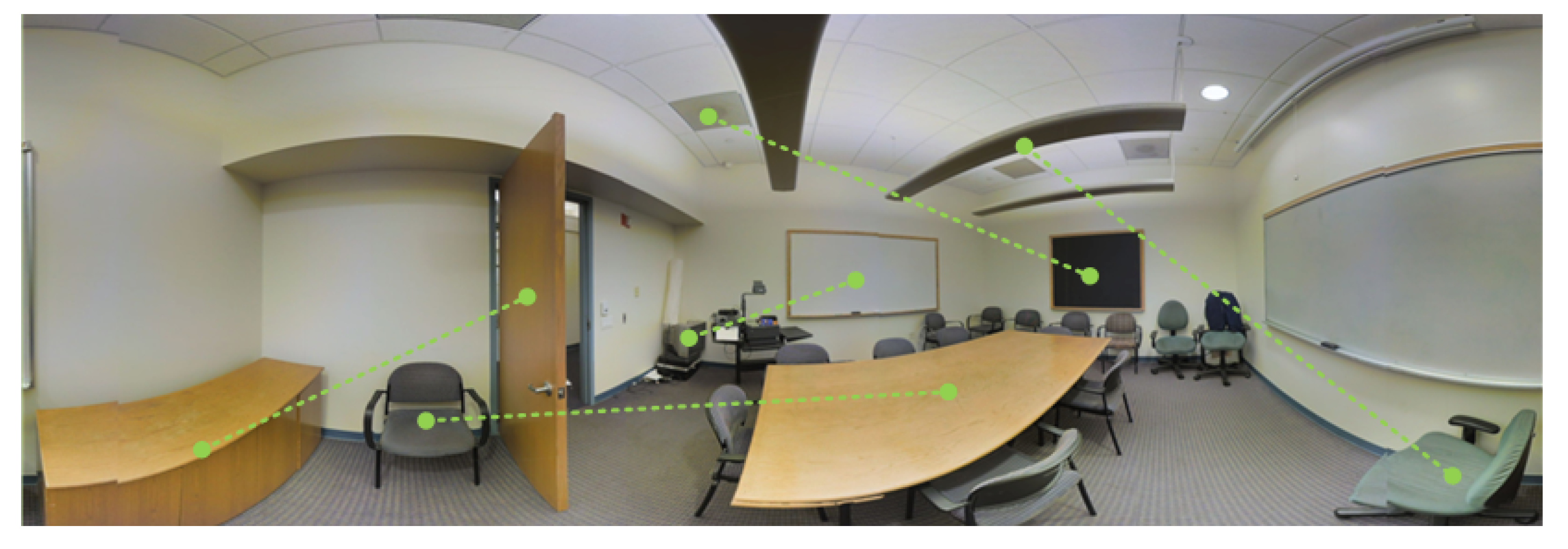
Thanks to the rapid development of deep learning, the 3D reconstruction of a room layout has gained new possibilities, and scholars have begun to use deep convolutional neural networks to explore 3D reconstruction problems. HorizonNet [5] proposed the combination of ResNet [6] and a recurrent neural network (RNN) for 3D room layout reconstruction. Wang et al. [7] proposed a method based on a convolution neural network for the task of predicting the surface normal from a single image. Intuitively, the problem of 3D room layout reconstruction should focus on the shape bias of the indoor layout instead of the texture bias. For example, the distance between two objects can be considered, as shown in Figure 1.
However, CNNs are limited by the problem of receptive fields; for example, a common convolution kernel is 3 × 3. Typical hidden layer feature sizes range from 256,512 to 1024, and the information felt by the 3 × 3 convolution kernel under the feature of these dimensions is very local. Increasing the size of the convolution kernel increases the receptive field, but it also brings about a large increase in the number of parameters and a delay in inference speed. For instance, suppose the size of the input feature is 64,384,64,64; we input this into a 24-layer depthwise convolution with a 13 × 13 kernel size, implemented with Pytorch, and with a latency of 600 ms [8]. Recently, Vision Transformer (ViT) [9], with its global receptive field and dynamic interaction capabilities, has been used to fully represent and model the context relationships in the image, achieving better results in many downstream tasks such as semantic segmentation and image classification. It is natural to think of a way to introduce ViT into 3D room layout reconstruction problems, using its shape sensitivity to better shape the layout prediction. However, drawbacks to the direct use of ViT for the 3D reconstruction of room layout remain: (1) The time complexity of calculation is high. The computation time complexity of the dot-product attention is , where L is the length of the input feature. (2) A large number of parameters. This not only makes training difficult, but also brings about the problem of gradient dissipation during gradient backpropagation. (3) Attention deficit. Although ViT has the advantage of a global receptive field, in theory, it has the problem of a limited receptive field in practice when analyzing its attention.
To solve the above problems, we propose a novel neural network named MreNet. Generally speaking, to make structural inferences about an indoor layout, we introduce dot-product attention into the model and obtain a global receptive field similar to ViT. To improve the inference speed of the model, we use sparse attention instead of full attention to calculate dot-product attention. To accelerate the speed of training and the mixing of features of different granularity, we propose a feature connection mechanism to connect different layers. Finally, we propose a novel structure based on a larger convolution kernel to enhance its sensitivity to local shape and address the attention deficit.
In general, the contributions of this paper are as follows:
- We propose a novel neural network named MreNet, based on ViT [9], to model the structural problem of the room layout. By using this architecture, we obtain a larger receptive field than the traditional convolutional neural networks, so we obtain a better modeling effect.
- We introduce a sparse attention mechanism to replace the traditional full attention mechanism in order to enhance the inference speed of the model and reduce the time complexity of operation.
- We propose an assistant structure that enhances the local large receptive field and introduce it into our model to enhance the shape sensitivity of the model.
- We propose a novel feature connection mechanism to solve the problem of the gradient disappearing in the process of training, and feature maps of different granularity can be obtained in different layers.
2. Related Work
In the following, we first review two main methods for 3D indoor reconstruction: traditional machine-learning-based methods and deep-learning-based methods. Then, we present a brief description of the vision transformer.
2.1. Methods Based on Traditional Machine Learning
Delage et al. [10] proposed a dynamic Bayesian network to identify the boundary between the floor and wall in each column of the image and solved some ambiguities in autonomous 3D reconstruction. The model could recognize the boundary between different objects in each column of the image by assuming the conjecture, in order to carry out 3D reconstruction. However, due to the well-known disadvantages of the Bayes method, its performance was hard to improve further, in terms of factors such as sensitivity to the representation of input data and poor performance in processing large datasets, etc. Lee et al. [2] generated the layout hypothesis based on the line segment set extracted from a single room image and could also identify the layout of the 3D structure of the building under the condition of occlusion and then select the most appropriate layout from it. However, they used a method based on line segments, and it was therefore difficult to provide global information on room layout. Ramalingam et al. [3] converted the room layout estimation problem into a conditional random field inference problem. They chose to use a simple and efficient voting mechanism to identify and classify connection points and then introduced the characteristics of connection points into a conditional random field inference problem, to estimate the layout of indoor scenes. Some subsequent studies also adopted similar methods, improving the extraction method of feature clues and the mechanism of generating the layout [4]. Most of the above studies used traditional machine learning methods, which are limited by the representation ability of the model, and the effect of 3D reconstruction is difficult to further improve.
2.2. Methods Based on Deep Learning
Mallya et al. [11] proposed a method for estimating the edge character of an indoor layout from a panoramic image, which could extract the edge of the room scene characteristic and used it to analyze the room layout, assuming that the edge referred to each plane’s intersecting lines, such as ceiling and metope, ground and metope of the line intersection curve, etc. They used a structured forest to extract the local information of the input image, and a full convolutional neural network to extract the global information of the input image to obtain the edge image, and then extracted its features and used a maximum margin classifier to estimate the room layout. Dasgupta et al. [12] proposed a new optimization framework based on a convolutional neural network, which could generate a room layout estimation with high accuracy in the face of complex room scenes. Lee et al. [13] proposed a network model with an encoder–decoder structure based on self-attention, which could predict the key points of an indoor layout. This method showed that an indoor layout estimation result and segmentation result could be obtained according to some specific sequence key points. AtlantaNet [14] proposed a neural network structure, which double-projected the original panoramic images to better encode the required modeling information. Recursive neural networks (RNNs) were used to capture remote geometric patterns, and custom training strategies based on domain-specific knowledge were utilized. Most of the deep-learning-based methods use a CNN as their backbone, but, being limited by the CNN’s smaller receptive field, their performance is hard to improve further.
2.3. Vision Transformer
Vision Transformer (ViT) [9] directly uses the pure transformer structure without combining it with a convolutional neural network. Vanilla ViT [9] has achieved good results in many image classification tasks. Specifically, it mainly adopts a method of converting pictures into tokens and introduces the concept of picture to patch in the original text. The input picture is divided into patches one by one, and then a flatten conversion is performed for each patch to transform it into an input structure, similar to Bert [15]. The Swin Transformer [16] makes use of a sliding window and hierarchical structure, making the Swin Transformer the new backbone in the field of machine vision, reaching the level of SOTA in image classification, target detection, semantic segmentation and other machine vision tasks. ConvMixer [17] uses a 9 × 9 convolution to replace the attention mechanism in ViT. The Pyramid Vision Transformer [18] proposes a feature pyramid structure based on Vision Transformer to accommodate downstream tasks requiring different feature densities and introduces sparse attention to solve computational complexity problems, but the proposed sparse attention is based on heuristics. The above work on ViT has achieved comparable or even better results than CNNs in many fields, but they also have problems: the number of model parameters is too large, and the training cost is too high. For example, if the number of parameters is limited, the performance of ViT is greatly weakened.
3. Methodology
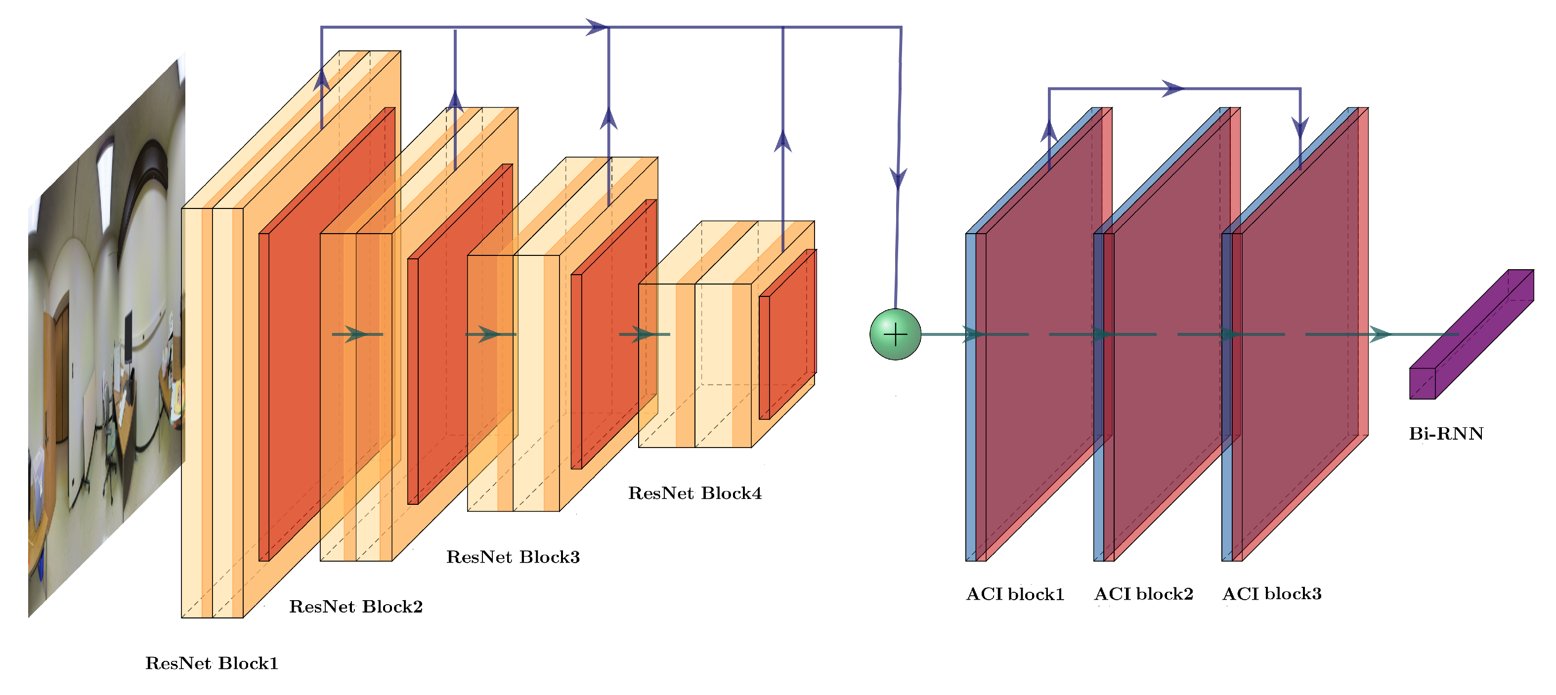
Aimed at solving the existing problems, we proposed a new neural network to enhance the effect of 3D indoor reconstruction, named Multiple Receptive Fields Enhanced Net (MreNet). The architectural design is shown in Figure 2.
The proposed MreNet consists of three main components, including ResNet-50 [6], an attention and convolution interaction (ACI) module, and LSTM. ResNet-50 and LSTM are similar to those used in HorizonNet [5]. Through experiments, we found that MreNet mainly benefited from the enhancement of the receptive field of the ACI module with regard to the improvement in the effect of 3D reconstruction. Therefore, the rest of this paper focuses on the ACI module. The ACI module mainly consists of three different parts: (1) the sparse attention layer; (2) the enhancement layer; and (3) the feature connection mechanism. Specifically, the sparse attention layer is responsible for modeling the indoor layout by using a global receptive field, while the enhancement layer uses a large convolution kernel to enhance the part that attention cannot cover in practice. The feature connection mechanism enables features of different granularity between different layers to interact, thus obtaining richer modeling effects.
3.1. ResNet for the Extraction of Features
We used ResNet-50 [6] as a feature extractor for the initial feature acquisition, similar to the one used in HorizonNet. The convolution kernel used in ResNet-50 has a sizes of 3 × 3 and 1 × 1, and the existence of receptive fields makes the feature granularity of different layers different. Intuitively, the 3D indoor reconstruction information they contain is also different. For example, shallow features may contain attributes such as texture and color, while deep features may contain shapes and relative relationships between objects with different orientations due to the increase in the number of receptive fields. We cached the outputs of different layers, and finally spliced the cached features of different granularity so that the obtained feature map was rich in these features. The detailed process of information transfer is shown in the following formulas.
where X denotes the origin input feature, is the ith block of ResNet, represents the output of the ith block of ResNet, ⊕ represents the concatenation operation and Y is the output of the whole ResNet.
3.2. ACI Module
ResNet is a combination of convolutional neural network layers based on two different convolutional kernels of different sizes. It has well-known limitations, such as the small size of a single receptive field, which is not conducive to capturing global features. Therefore, we started from its limitations and designed a new neural network that could make up for its shortcomings to enhance the 3D room reconstruction. In this section, we describe the ACI module from the following perspectives: (1) the inputs and outputs of the module, (2) the sparse attention, (3) the enhancement layer and (4) the shortcut.
3.2.1. Input and Output of the Overall ACI Module
The input and output operations of the ACI module are shown in Figure 2. In practice, we made three copies of the output features from ResNet after normalization [19]. We then calculated them as Q, K and V for the sparse attention, similar to the full attention in Transformer [20], but with a difference in the amount of computation. The formula of the vanilla full dot-product attention is as follows. We introduce our sparse dot-product attention in the next section.
where
where , , and are the projections, and is the dimension of the subfeature.
We then put the output of the sparse dot-product attention layer through a layer of dropout, which randomly dropped some neurons to enhance the robustness of the model and avoid overfitting. Furthermore, the output was input into the enhancement layer to enrich the feature information. Finally, we propagated the resulting output to the MLP, which was similar to the one used in ViT.
3.2.2. Sparse Attention Layer
The original calculation of self-attention requires a large amount of computation, and its time complexity is . In the training phase, this requires a great deal of calculation, so the training time is too long and is difficult to deploy in practical applications. In the inference stage, due to the problem of computational complexity, the inference is slow, thus resulting in a low efficiency in practical applications. In the actual operation, we output the reconstructed attention of the 3D room layout and found that attention was sparsely distributed, and that many of the dot-product operations did not have a great influence on the result. Inspired by Informer [21], we used a similar sparse attention mechanism in each of our layers. This reduced the overall time complexity of the operation to . The sparse attention formulas are as follows:
where ⊕ is the concatenation operation, is the top Q with the highest score, denotes the operation of the mean and is the output of the single sparse attention layer. The other variables are the same as those of the original formula, which we described above.
3.2.3. Enhancement Layer
ViT can theoretically model the global relationship of features and capture feature interactions over long distances. However, many scholars have found that there is a lack of attention in actual operation. Some works provided empirical results to demonstrate this. Inspired by these works, we viewed the problem from another angle. Since ViT can generate suboptimal levels of global modeling, can we design a new structure to enhance its utility rather than replace it? To this end, we designed a new structure to enhance the sensitivity of local receptive fields. Specifically, we input the output of the multiplex attention into two convolution layers with large convolution kernels to obtain the output of the receptive field enhancement. In our work, we used convolution kernels of and . Convolution kernels of different sizes can also be used in different tasks, which is easy to achieve in practice. In addition, inspired by the guideline for the use of large-scale convolution kernels in [8], we output multiattention outputs through a convolution and added the output results from two convolution layers with and convolution kernels. Specifically, the output process of the enhancement layer is shown below:
where X denotes the input of the enhancement layer, denotes the convolution layer with a convolution kernel, denotes the convolution layer with a convolution kernel and denotes the convolution layer with a convolution kernel.
3.2.4. Feature Connection Mechanism
In the deep neural network, the feature granularity between different layers is different. Generally speaking, features at lower levels tend to be fine-grained, which means they can more easily grasp fine features such as textures, corners, furniture details and so on. Features at higher levels tend to be coarser in granularity, which means they focus on broader information than features at lower levels, such as the shape of the indoor furniture, the distance between the center of the sofa and the floor and the relative position of the ceiling and walls. To better capture the feature information between different layers and to not lose the features of different granularity of each layer, we adopted a hierarchical connection mode for feature interaction between different layers. In addition to the above-mentioned benefits brought by the fusion of features with different granularity, we also observed an improvement of the gradient disappearance in the experiment, thus accelerating the convergence speed and strengthening the convergence effect in the training, similar to that found in [22]. Specifically, our connection mode was as follows:
where X denotes the input of the ACI module and denotes the ith of the ACI module.
3.3. The Use of a Recurrent Neural Network for the Convergence of Features
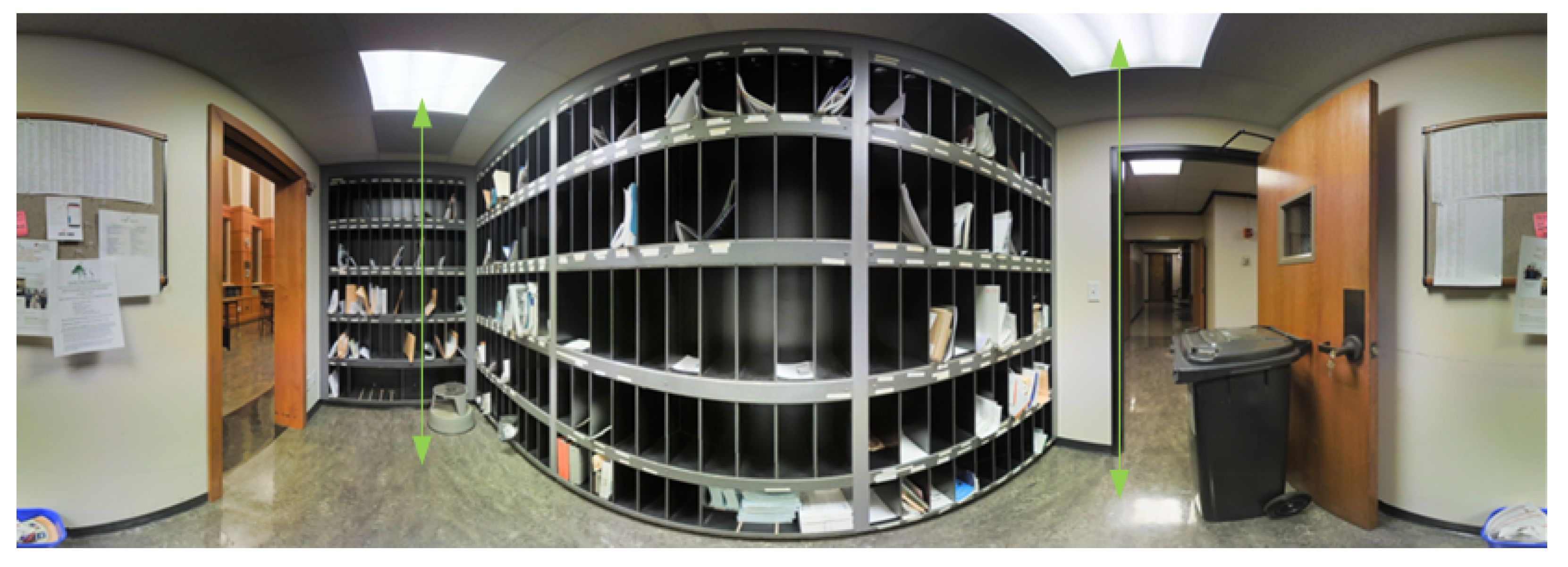
Intuitively, each part of the room has a relationship with the others. For example, if we know where the floor is, we know the ceiling is probably on the other side of the floor. Conversely, knowing the position of the ceiling, we also know that the floor is probably on the other side of it, as shown in Figure 3.
To this end, we used a bidirectional RNN [23] to capture bidirectional relationships between different positions. The bidirectional RNN we used was as follows:
where denotes the positive weight matrix corresponding to the input, denotes the positive weight matrix corresponding to the output at the last moment, denotes the positive bias, denotes the inverse weighting matrix corresponding to the input, denotes the inverse weighting matrix corresponding to the previous output, B2 denotes the inverse bias, f denotes the activation function, U denotes the weight matrix of the output mixing information, c denotes the final mixing bias and g denotes the final activation function.
4. Experimental Results and Discussion
4.1. Experimental Settings
Environment setting: In our experiment, we used a server equipped with an Intel Xeon E5-2650 V2 CPU and GeForce GTX 3090 GPU for training. The network was implemented in PyTorch.
Datasets: In terms of datasets, we used the PanoContext [24] and Stanford 2D-3D [25] datasets to train and evaluate the proposed network model. The PanoContext dataset contains 500 annotated cuboid layouts, including indoor environments such as bedrooms and living rooms. Since the resolution of panoramic images in the original PanoContext dataset was 9104 × 4552, which did not meet the requirements of the model in this paper for input images, the resolution of all images in the PanoContext dataset was changed to 1024 × 512 in this paper.
Hyperparameter setting: We employed the Adam optimizer [26] to train the network for 300 epochs and a learning rate of 0.0003. The training process is analyzed in the following sections. We set the number of sparse attention layers as three and the number of enhancement layers as three. We also tested different numbers of sparse attention layers and enhancement layers, e.g., six and nine. With the increase of the number of layers, there was no significant improvement, but the training time was greatly increased. We set the batch size of the training as four and the batch size of the validation as two. Through experiments, we found that different batch sizes did not cause visible differences, but a big batch size easily caused an out-of-memory error from the GPU.
Training time: The training time overhead of MreNet was 0.0184 h per epoch and that of HorizonNet was 0.0179 h per epoch. Due to the introduction of the multihead attention of Vision Transformer into MreNet which brought extra parameters, the time consumption of MreNet increased slightly. However, compared to HorizonNet, considering that MreNet could achieve more than 0.68% of improvement in 3D IoU, the 0.027% time overhead was tiny.
4.2. Evaluation Metrics
In this section, we present the three metrics used to evaluate the proposed MreNet, including 3D intersection over union (IoU), corner error and pixel error. We describe the three metrics next.
IoU is the measurement of the accuracy of the test results. The object to be detected has a truth box, namely the ground truth. It is necessary to artificially mark the general range of the object with a rectangular box on the pictures in the dataset. In the evaluation of an algorithm, the algorithm first needs to be used to detect the image, then the prediction box of the corresponding object generated by the algorithm can be obtained, and then the IoU index between the prediction box and the truth box is calculated.
The larger the value of the IoU, the better the consistency between the prediction box and the truth box, and the higher the accuracy of the algorithm. The corresponding mathematical formula is as follows:
where denotes the area of the prediction box generated by the neural network and denotes the area of the real box.
The 3D IoU in this paper refers to the result of dividing the area of the intersection and the union area between the 3D layout and the marked real layout generated by the layout estimation based on the proposed method. The formula is as follows:
where denotes the volume of the generated 3D layout estimated using the neural network and denotes the volume of the actual 3D layout.
Corner error denotes the average Euclidean distance between the predicted angle and the true angle. The calculation formula of the corner error is as follows:
where denotes the value of the corner error, denotes the average Euclidean distance, H denotes the distance between the predicted angle and the real angle and W denotes the width of the input panoramic image.
Pixel error refers to the average pixel error between the predicted layout and the real layout, and its mathematical calculation formula is as follows:
where denotes the pixel values of the structural lines, such as walls and ceilings in the generated 3D layout, denotes the pixel value of each structure line in a real 3D layout and denotes the pixel error.
It can be inferred that if the predicted pixel value is equal to the real pixel value, the value of is zero. Conversely, if the predicted pixel value is not equal to the real pixel value, the value is one. H denotes the height of the input panoramic image and W denotes the width of the input panoramic image.
4.3. Convergence Analysis
Convergence is a measure of the stability and reliability of deep learning neural networks for 3D reconstruction, so it is important to test the convergence and generalization of deep learning models.
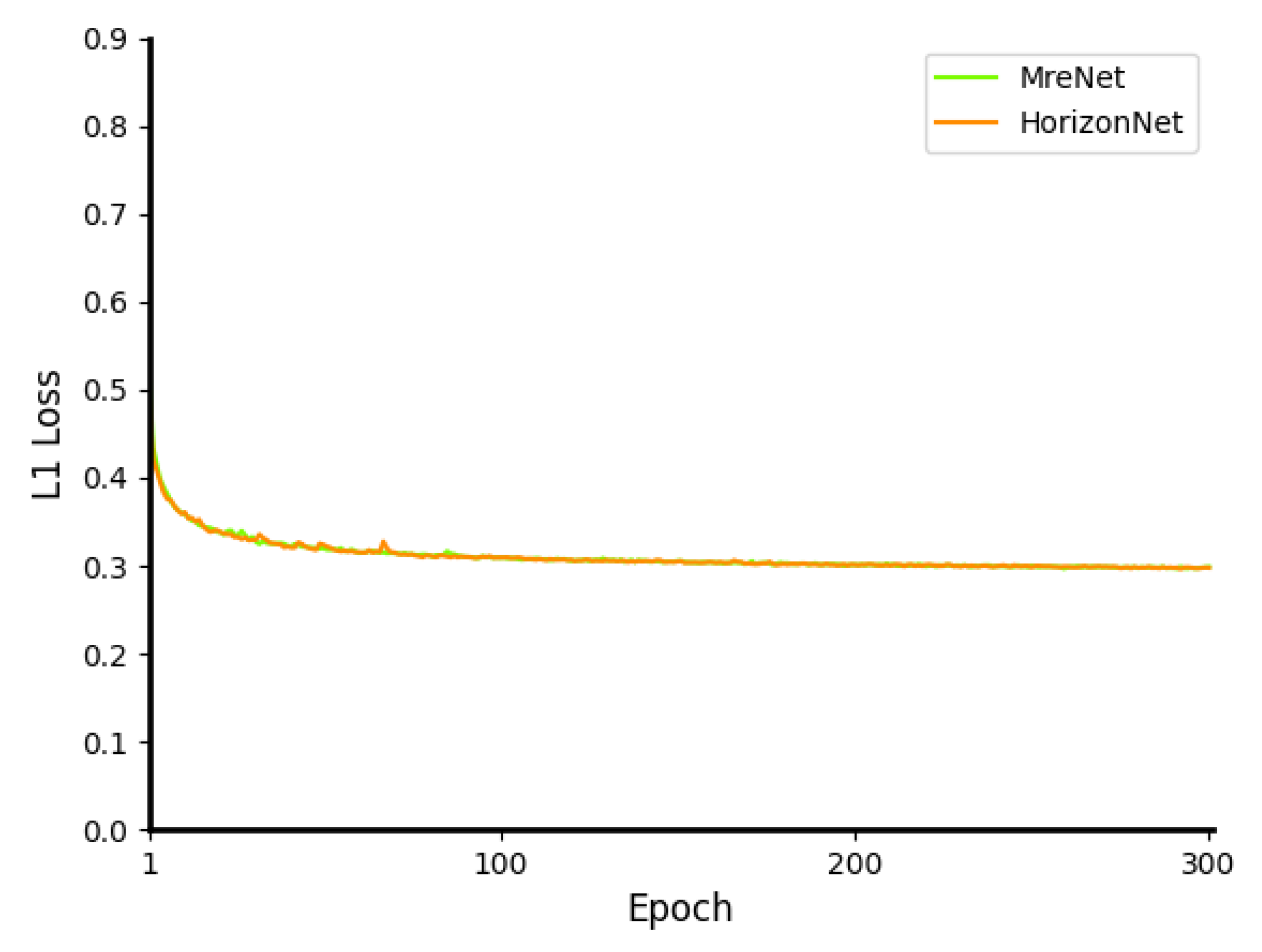
To fully verify the reliability of our MreNet model, we adopted the state-of-the-art HorizonNet [5] as the control. As shown in Figure 4, from the 300 epochs of training, both MreNet and HorizonNet converged towards good performance, and they converged at almost the same rate. However, in terms of stability, MreNet was better than HorizonNet since in the first 100 epochs in training, MreNet had fewer peaks in the green curve in Figure 4. Furthermore, we made a statistical analysis of the loss during training. In the final smooth 250–300 epochs, the loss variance of MreNet was while that of HorizonNet reached .
Through the above experimental analysis, the convergence of the proposed MreNet was proved.
4.4. Ablation Study
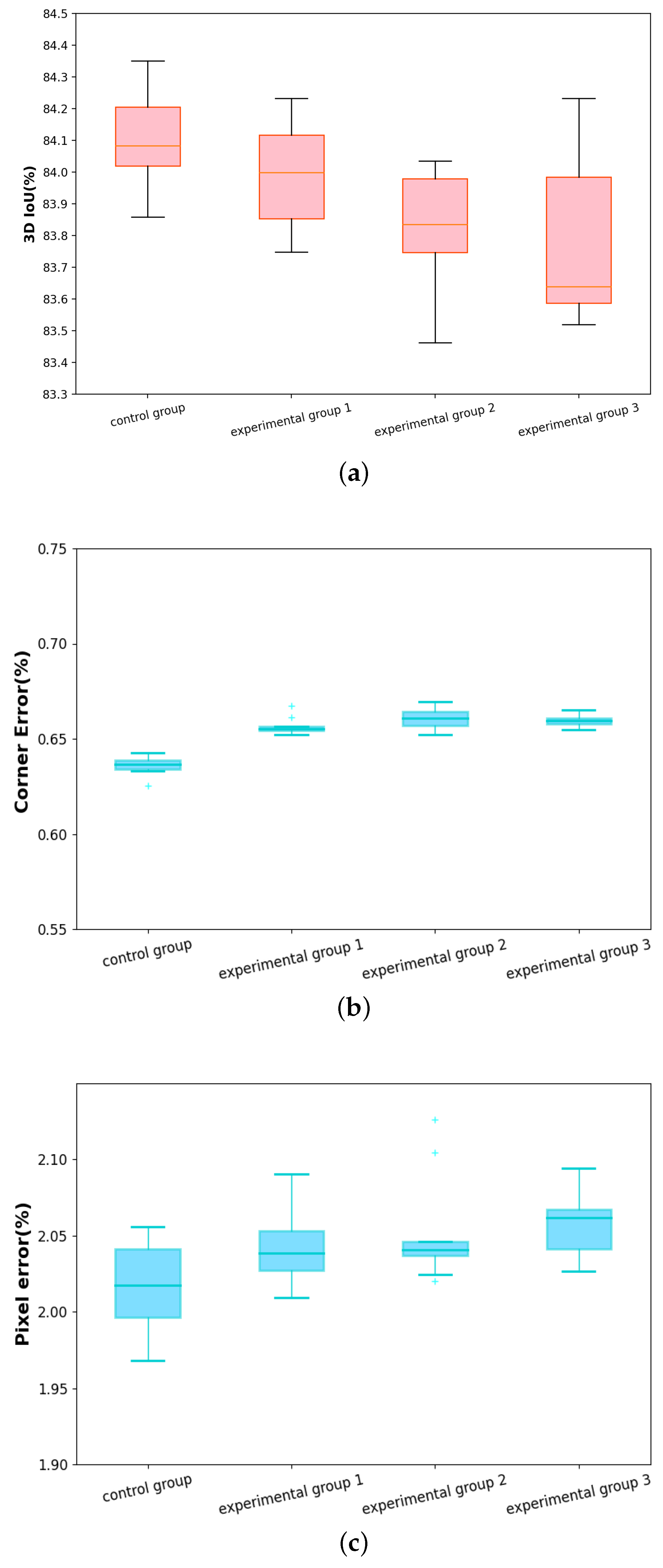
We performed an ablation study to verify the performance of MreNet. First, we took the complete version of MreNet as the control group, MreNet without the enhancement layer as experimental group 1, MreNet without the feature connection as experimental group 2 and MreNet without the sparse attention layer as experimental group 3. We trained and tested them on the PanoContext dataset + Stanford-2D3D. As shown in Figure 5, in terms of 3D IoU, the experimental groups 1, 2 and 3 achieved 83.88%, 83.82% and 83.77%, respectively, while the control group achieved 84.09%. Concerning the corner error, the experimental groups 1, 2 and 3 reached 0.657%, 0.659% and 0.661%, respectively, while the control group achieved 0.639%. Regarding the pixel error, the experimental groups 1, 2 and 3 yielded 2.047%, 2.049% and 2.051%, respectively, while the control group had a pixel error of 2.030%. We also conducted some statistical hypothesis tests. For the two-sample heteroscedastic assumption-test, the 3D IoU result for the control group with experimental groups 1, 2 and 3 was 0.0051, 0.0043 and 0.0049, respectively. The results for corner errors were 0.0008, 0.004 and 0.002. The results for pixel error were 0.043, 0.029 and 0.0031.
In conclusion, as the complete version of MreNet achieved good performance from these three metrics, the necessity of the sparse attention layer, enhancement layer and feature connection were verified.
4.5. Quantitative Evaluation
Our approach was evaluated on the three above-mentioned standard metrics: (1) 3D IoU, (2) corner error and (3) pixel error. The descriptions of these three metrics were introduced in Section 3.1, so they are not repeated in this section. The results of different approaches are summarized in Table 1, Table 2 and Table 3. The input resolution of HorizonNet and LayoutNet [27] was . Our approach achieved state-of-the-art performance and outperformed existing methods under all settings. The mean of the three indicators (3D IoU, corner error and pixel error) are presented after each experiment was repeated five times. The T-test was the two-sample heteroscedastic assumption for HorizonNet and MreNet.
4.6. Qualitative Results
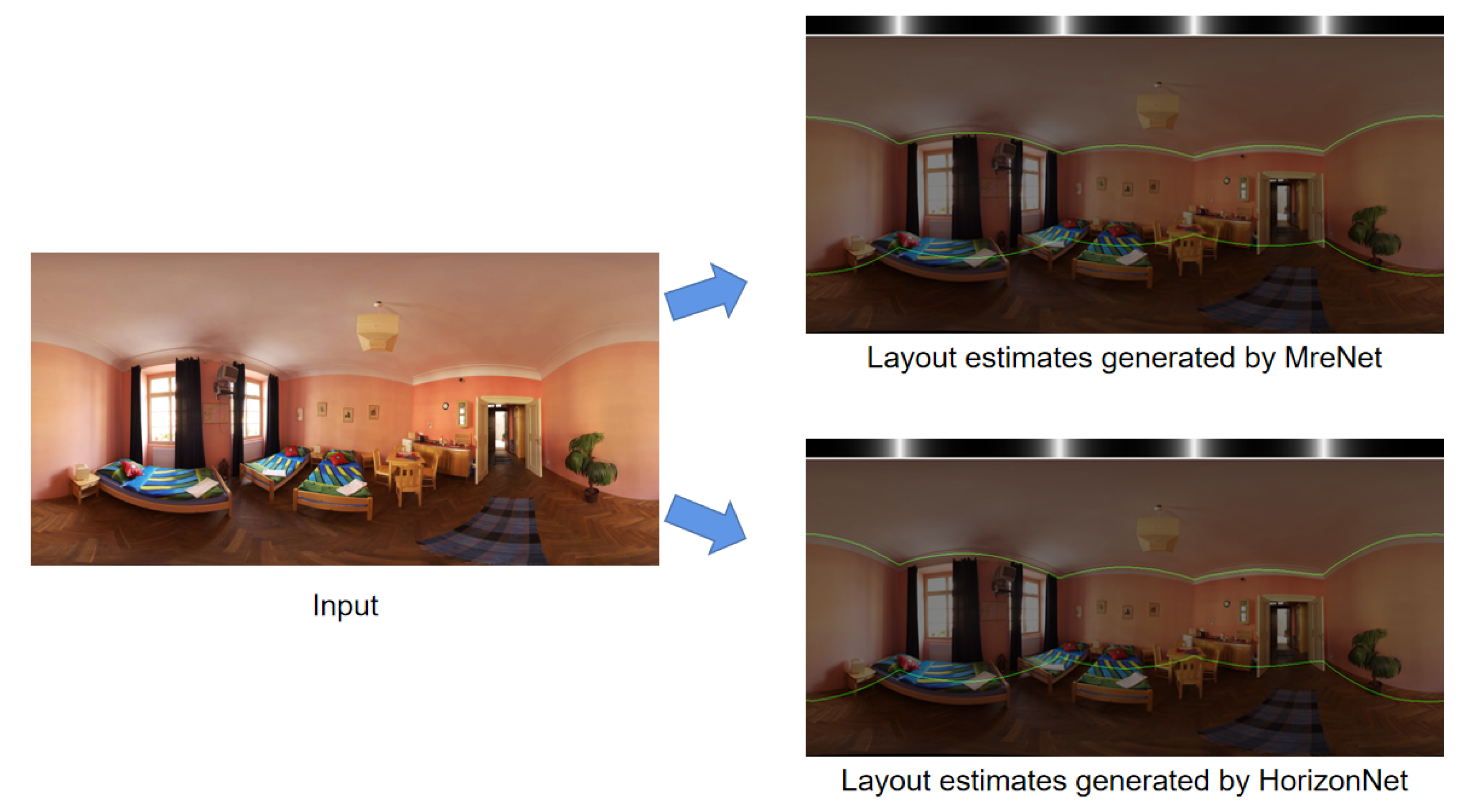
To test the actual effect of the reconstruction of a room layout, we took the best models obtained from MreNet and HorizonNet to estimate the layout of the panoramic image of the same rooms. The obtained layout estimation results are shown in Figure 6. It is obvious from the image that the layout estimation generated by the MreNet is more accurate in predicting the boundary of each plane, especially for the estimation of the location of the boundary between the ceiling and the wall.
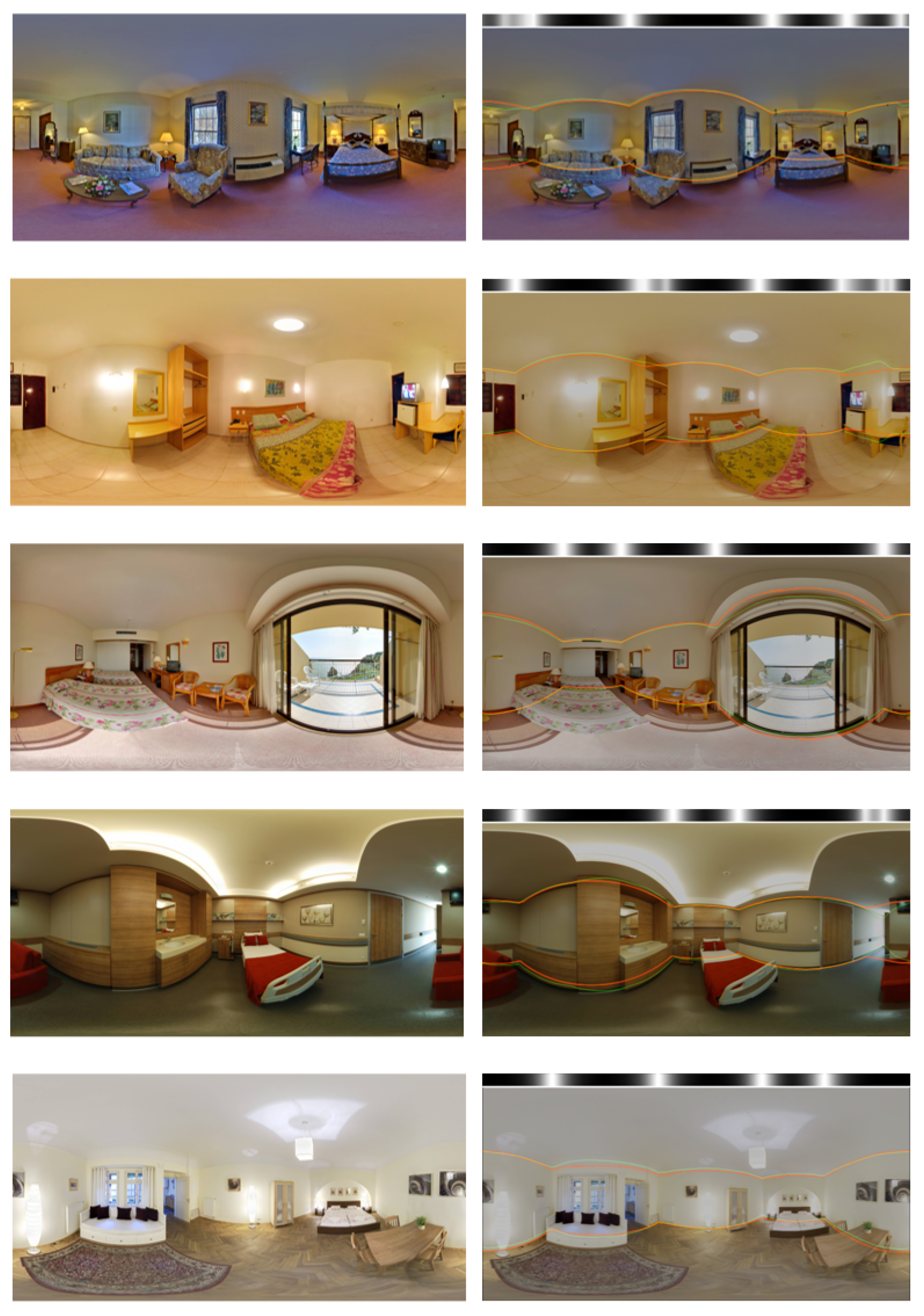
To further verify the correctness of this conclusion, we used multiple panoramic images for comparative experiments, and the results obtained are depicted in Figure 7 where the green lines are layout estimated by MreNet while the orange lines are for HorizonNet. It can be seen from the image that although both can perform relatively accurate layout estimation, MreNet can more accurately fit the boundary position of each plane, such as the position of the boundary between the ceiling and wall. In addition, MreNet can better estimate the location of some plane boundaries obscured in the figure by indoor furniture.
4.7. Discussions
Compared to the-state-of-art methods, e.g., HorizonNet and PanoContext, MreNet had a higher modeling capability, in terms of 3D IoU (%), and the highest improvement was 0.68% and 14.72%, respectively. Considering the rate of convergence, in 50 stable epochs, the loss variance of MreNet was while that of HorizonNet was . We attributed these contributions mainly to the enlarged receptive field. Intuitively, the more receptive fields, the more feature information is obtained. Moreover, our experiments showed that the proposed approach outperformed the existing approaches on all three standard metrics.
Although the proposed sparse attention layer and feature connection mechanism greatly improved the estimating efficiency and the proposed enhancement layer enabled the MreNet to have a large receptive field, compared with a CNN-based model, e.g., HorizonNet, MreNet’s time consumption increased a bit. Therefore, our next research direction is to combine the speed of CNNs and the global modeling ability of the attention module.
5. Conclusions
In this paper, we studied the problem of reconstructing the 3D room layout from a single RGB panoramic image. A novel approach based on our high-efficiency network structure was developed, which obtained a global receptive field. In addition, our proposed feature connection mechanism significantly enhanced the speed of training and mixing features. There are several possible directions that can be explored for future works. Firstly, developing efficient techniques for complex, general layouts is an interesting issue to be investigated. In actual application, indoor layouts are more sophisticated and often possess features that are in conflict with the “Manhattan world” assumption, such as arches. Secondly, the incorporation of object classification/detection for a better understanding of 3D scenes is another interesting issue to be studied.
Author Contributions
Funding acquisition, W.L.; investigation, Y.S.; methodology, B.X.; project administration, B.X., Y.S. and W.L.; resources, B.X. and Y.S.; software, X.M. and Z.L.; supervision, B.X., Y.S. and W.L.; validation, Y.S.; writing—original draft, X.M. and Z.L.; writing—review and editing, B.X. and W.L. All authors have read and agreed to the published version of the manuscript.
Funding
This research was funded by the Fundamental Research Funds for the Central Universities, 3072022TS0605, 3072022YY0601, 3072022CF0601, and the State Administration of Foreign Expert Affairs, G2021180021L.
Institutional Review Board Statement
Not applicable.
Informed Consent Statement
Not applicable.
Data Availability Statement
Not applicable.
Conflicts of Interest
The authors declare no conflict of interest.
References
- Bhuyan, M.K. Computer Vision and Image Processing: Fundamentals and Applications; CRC Press: Boca Raton, FL, USA, 2019. [Google Scholar]
- Lee, D.C.; Hebert, M.; Kanade, T. Geometric reasoning for single image structure recovery. In Proceedings of the 2009 IEEE Conference on Computer Vision and Pattern Recognition, Miami, FL, USA, 20–25 June 2009; IEEE: Piscataway, NJ, USA, 2009; pp. 2136–2143. [Google Scholar]
- Ramalingam, S.; Pillai, J.K.; Jain, A.; Taguchi, Y. Manhattan junction catalogue for spatial reasoning of indoor scenes. In Proceedings of the IEEE Conference on Computer Vision and Pattern Recognition, Portland, OR, USA, 23–28 June 2013; pp. 3065–3072. [Google Scholar]
- Wang, H.; Gould, S.; Koller, D. Discriminative learning with latent variables for cluttered indoor scene understanding. In Proceedings of the European Conference on Computer Vision, Heraklion, Greece, 5–11 September 2010; Springer: Berlin/Heidelberg, Germany, 2010; pp. 497–510. [Google Scholar]
- Sun, C.; Hsiao, C.W.; Sun, M.; Chen, H.T. Horizonnet: Learning room layout with 1d representation and pano stretch data augmentation. In Proceedings of the IEEE/CVF Conference on Computer Vision and Pattern Recognition, Long Beach, CA, USA, 15–20 June 2019; pp. 1047–1056. [Google Scholar]
- He, K.; Zhang, X.; Ren, S.; Sun, J. Deep residual learning for image recognition. In Proceedings of the IEEE Conference on Computer Vision and Pattern Recognition, Las Vegas, NV, USA, 27–30 June 2016; pp. 770–778. [Google Scholar]
- Wang, X.; Fouhey, D.; Gupta, A. Designing deep networks for surface normal estimation. In Proceedings of the IEEE Conference on Computer Vision and Pattern Recognition, Boston, MA, USA, 7–12 June 2015; pp. 539–547. [Google Scholar]
- Ding, X.; Zhang, X.; Han, J.; Ding, G. Scaling up your kernels to 31 × 31: Revisiting large kernel design in cnns. In Proceedings of the IEEE/CVF Conference on Computer Vision and Pattern Recognition, New Orleans, LA, USA, 9–16 November 2022; pp. 11963–11975. [Google Scholar]
- Dosovitskiy, A.; Beyer, L.; Kolesnikov, A.; Weissenborn, D.; Zhai, X.; Unterthiner, T.; Dehghani, M.; Minderer, M.; Heigold, G.; Gelly, S.; et al. An image is worth 16 × 16 words: Transformers for image recognition at scale. arXiv 2020, arXiv:2010.11929. [Google Scholar]
- Delage, E.; Lee, H.; Ng, A.Y. A dynamic bayesian network model for autonomous 3d reconstruction from a single indoor image. In Proceedings of the 2006 IEEE Computer Society Conference on Computer Vision and Pattern Recognition (CVPR’06), New York, NY, USA, 17–22 June 2006; IEEE: Piscataway, NJ, USA, 2006; Volume 2, pp. 2418–2428. [Google Scholar]
- Mallya, A.; Lazebnik, S. Learning informative edge maps for indoor scene layout prediction. In Proceedings of the IEEE International Conference on Computer Vision, Santiago, Chile, 7–13 December 2015; pp. 936–944. [Google Scholar]
- Dasgupta, S.; Fang, K.; Chen, K.; Savarese, S. Delay: Robust spatial layout estimation for cluttered indoor scenes. In Proceedings of the IEEE Conference on Computer Vision and Pattern Recognition, Las Vegas, NV, USA, 27–30 June 2016; pp. 616–624. [Google Scholar]
- Lee, C.Y.; Badrinarayanan, V.; Malisiewicz, T.; Rabinovich, A. Roomnet: End-to-end room layout estimation. In Proceedings of the IEEE International Conference on Computer Vision, Venice, Italy, 22–29 October 2017; pp. 4865–4874. [Google Scholar]
- Pintore, G.; Agus, M.; Gobbetti, E. AtlantaNet: Inferring the 3D Indoor Layout from a Single 360∘ Image Beyond the Manhattan World Assumption. In Proceedings of the European Conference on Computer Vision, Glasgow, UK, 23–28 August 2020; Springer: Berlin/Heidelberg, Germany, 2020; pp. 432–448. [Google Scholar]
- Devlin, J.; Chang, M.W.; Lee, K.; Toutanova, K. Bert: Pre-training of deep bidirectional transformers for language understanding. arXiv 2018, arXiv:1810.04805. [Google Scholar]
- Liu, Z.; Lin, Y.; Cao, Y.; Hu, H.; Wei, Y.; Zhang, Z.; Lin, S.; Guo, B. Swin transformer: Hierarchical vision transformer using shifted windows. In Proceedings of the IEEE/CVF International Conference on Computer Vision, Montreal, BC, Canada, 11–17 October 2021; pp. 10012–10022. [Google Scholar]
- Trockman, A.; Kolter, J.Z. Patches are all you need? arXiv 2022, arXiv:2201.09792. [Google Scholar]
- Wang, W.; Xie, E.; Li, X.; Fan, D.P.; Song, K.; Liang, D.; Lu, T.; Luo, P.; Shao, L. Pyramid vision transformer: A versatile backbone for dense prediction without convolutions. In Proceedings of the IEEE/CVF International Conference on Computer Vision, Montreal, BC, Canada, 11–17 October 2021; pp. 568–578. [Google Scholar]
- Ba, J.L.; Kiros, J.R.; Hinton, G.E. Layer normalization. arXiv 2016, arXiv:1607.06450. [Google Scholar]
- Vaswani, A.; Shazeer, N.; Parmar, N.; Uszkoreit, J.; Jones, L.; Gomez, A.N.; Kaiser, Ł.; Polosukhin, I. Attention is all you need. Adv. Neural Inf. Process. Syst. 2017, 30, 1–11. [Google Scholar]
- Zhou, H.; Zhang, S.; Peng, J.; Zhang, S.; Li, J.; Xiong, H.; Zhang, W. Informer: Beyond efficient transformer for long sequence time-series forecasting. In Proceedings of the AAAI Conference on Artificial Intelligence, Virtual, 2–9 February 2021; Volume 35, pp. 11106–11115. [Google Scholar]
- Srivastava, R.K.; Greff, K.; Schmidhuber, J. Training very deep networks. Adv. Neural Inf. Process. Syst. 2015, 28, 1–9. [Google Scholar]
- Schuster, M.; Paliwal, K.K. Bidirectional recurrent neural networks. IEEE Trans. Signal Process. 1997, 45, 2673–2681. [Google Scholar] [CrossRef] [Green Version]
- Zhang, Y.; Song, S.; Tan, P.; Xiao, J. Panocontext: A whole-room 3d context model for panoramic scene understanding. In Proceedings of the European Conference on Computer Vision, Zurich, Switzerland, 6–12 September 2014; Springer: Berlin/Heidelberg, Germany, 2014; pp. 668–686. [Google Scholar]
- Armeni, I.; Sax, S.; Zamir, A.R.; Savarese, S. Joint 2d-3d-semantic data for indoor scene understanding. arXiv 2017, arXiv:1702.01105. [Google Scholar]
- Kingma, D.P.; Ba, J. Adam: A method for stochastic optimization. arXiv 2014, arXiv:1412.6980. [Google Scholar]
- Zou, C.; Colburn, A.; Shan, Q.; Hoiem, D. Layoutnet: Reconstructing the 3d room layout from a single rgb image. In Proceedings of the IEEE Conference on Computer Vision and Pattern Recognition, Salt Lake City, UT, USA, 18–22 June 2018; pp. 2051–2059. [Google Scholar]
Figure 1.
The relationships between objects and the room layout.

Figure 2.
Architecture of the MreNet.

Figure 3.
Correspondence between the ceiling and floor.

Figure 4.
Convergence behavior of MreNet and HorizonNet.

Figure 5.
Ablation study for MreNet. (a) is for 3D IoU, (b) is for corner error (CE) and (c) is the result of pixel error (PE).
Figure 5.
Ablation study for MreNet. (a) is for 3D IoU, (b) is for corner error (CE) and (c) is the result of pixel error (PE).

Figure 6.
Layout estimates generated by MreNet and HorizonNet.

Figure 7.
Multiple layout estimates generated by MreNet (green) and HorizonNet (orange).


Table 1.
Quantitative results of cuboid layout estimation evaluated on the PanoContext [24] dataset. Our approach outperforms all listed methods under all settings.
Table 1.
Quantitative results of cuboid layout estimation evaluated on the PanoContext [24] dataset. Our approach outperforms all listed methods under all settings.
| Method | 3D IoU (%) | Corner Error (%) | Pixel Error (%) |
|---|---|---|---|
| Training on PanoContext dataset | |||
| PanoContext | 67.51 | 1.57 | 4.49 |
| HorizonNet | 82.11 | 0.79 | 2.26 |
| MreNet | 82.23 | 0.79 | 2.24 |
| T-test | 0.002 | 0.0164 | 0.07 |
| Training on PanoContext + Stanford-2D3D datasets | |||
| HorizonNet | 83.40 | 0.72 | 2.03 |
| MreNet | 84.08 | 0.67 | 1.98 |
| T-test | 0.048 | 0.0217 | 0.007 |
Table 2.
Quantitative results of cuboid layout estimation evaluated on the Stanford-2D3D [25] dataset. Our approach outperforms all listed methods under all settings.
Table 2.
Quantitative results of cuboid layout estimation evaluated on the Stanford-2D3D [25] dataset. Our approach outperforms all listed methods under all settings.
| Method | 3D IoU (%) | Corner Error (%) | Pixel Error (%) |
|---|---|---|---|
| Training on PanoContext dataset | |||
| HorizonNet | 75.43 | 0.94 | 3.21 |
| MreNet | 75.55 | 0.94 | 3.18 |
| T-test | 0.004 | 0.023 | 0.048 |
| Training on Stanford-2D3D dataset | |||
| HorizonNet | 79.57 | 0.75 | 2.44 |
| MreNet | 79.89 | 0.70 | 2.38 |
| T-test | 0.047 | 0.015 | 0.041 |
| Training on PanoContext + Stanford-2D3D datasets | |||
| HorizonNet | 83.86 | 0.65 | 2.10 |
| MreNet | 84.11 | 0.62 | 2.06 |
| T-test | 0.037 | 0.031 | 0.034 |
Table 3.
Quantitative results of cuboid layout estimation evaluated on the Stanford-2D3D [25]+ PanoContext dataset [24]. Our approach outperforms all listed methods under all settings.
| Method | 3D IoU (%) | Corner Error (%) | Pixel Error (%) |
|---|---|---|---|
| Training on PanoContext + Stanford-2D3D datasets | |||
| HorizonNet | 83.76 | 0.67 | 2.07 |
| MreNet | 84.09 | 0.64 | 2.03 |
| T-test | 0.021 | 0.027 | 0.044 |
Publisher’s Note: MDPI stays neutral with regard to jurisdictional claims in published maps and institutional affiliations. |
© 2022 by the authors. Licensee MDPI, Basel, Switzerland. This article is an open access article distributed under the terms and conditions of the Creative Commons Attribution (CC BY) license (https://creativecommons.org/licenses/by/4.0/).
Share and Cite
MDPI and ACS Style
Xu, B.; Sun, Y.; Meng, X.; Liu, Z.; Li, W. MreNet: A Vision Transformer Network for Estimating Room Layouts from a Single RGB Panorama. Appl. Sci. 2022, 12, 9696. https://0-doi-org.brum.beds.ac.uk/10.3390/app12199696
AMA Style
Xu B, Sun Y, Meng X, Liu Z, Li W. MreNet: A Vision Transformer Network for Estimating Room Layouts from a Single RGB Panorama. Applied Sciences. 2022; 12(19):9696. https://0-doi-org.brum.beds.ac.uk/10.3390/app12199696
Chicago/Turabian StyleXu, Bing, Yaohui Sun, Xiangxu Meng, Zhihan Liu, and Wei Li. 2022. "MreNet: A Vision Transformer Network for Estimating Room Layouts from a Single RGB Panorama" Applied Sciences 12, no. 19: 9696. https://0-doi-org.brum.beds.ac.uk/10.3390/app12199696
Note that from the first issue of 2016, this journal uses article numbers instead of page numbers. See further details here.