Developing Predictive Models of Collapse Settlement and Coefficient of Stress Release of Sandy-Gravel Soil via Evolutionary Polynomial Regression

Abstract

The collapse settlement of granular soil, which brings about considerable deformations, is an important issue in geotechnical engineering. Several factors are involved in this phenomenon, which makes it difficult to predict. The present study aimed to develop a model to predict the collapse settlement and coefficient of stress release of sandy gravel soil through evolutionary polynomial regression (EPR). To achieve this, a dataset containing 180 records obtained from a large-scale direct shear test was used. In this study, five models were developed with the secant hyperbolic, tangent hyperbolic, natural logarithm, exponential, and sinusoidal inner functions. Using sand content (SC), normal stress (${\sigma }_n$), shear stress level (SL), and relative density (Dr) values, the models can predict the collapse settlement (∆H) and coefficient of stress release (CSR). The results indicated that the models developed with the exponential functions were the best models. With these models, the values of $R^2$ for training, testing, and all data in the prediction of collapse settlement were 0.9759, 0.9759, and 0.9757, respectively, and the values of $R^2$ in predicting the coefficient of stress release were 0.9833, 0.9820, and 0.9833, respectively. The sensitivity analysis also revealed that the sand content (SC) and relative density (Dr) parameters had the highest and lowest degrees of importance in predicting collapse settlement. In contrast, the Dr and SC parameters showed the highest and lowest degrees of importance in predicting the coefficient of stress release. Finally, the conducted parametric study showed that the developed models were in line with the results of previous studies.

1. Introduction

Since the second half of the 19th century, considerable attention has been paid to the use of coarse-grained soil in the construction of embankment dams. Then, improvements in the density methods and the use of coarse-grained soil meant that engineers were able to design and construct higher rockfill dams [1]. In order to control the functions of dams, their behaviour must be examined at the time of construction, and considerable data need to be gathered. Observations reveal that, with the first impoundment or heavy rain, not only long-term deformation (creep) [2] but also sudden settlements occur [3]. Sudden settlement during the first impoundment is a salient feature of central core clay dams with rockfill shells. This sudden settlement, which is referred to as collapse settlement, is ascribed to the impacts of floods in the upstream rockfill [4]. Collapse settlement is a dangerous geotechnical phenomenon that can damage dams and their equipment. However, it is hard to predict the collapses resulting from collapsible soil for various reasons, such as soil deformability, the degree of saturation, and the variable loading conditions [5].

Previous studies have indicated that most soils can be exposed to collapse [6,7,8,9]. In other words, if poorly graded unsaturated soil is excessively saturated under the loading process, it is likely to collapse. However, there must be poor binding between the grains for it to be destroyed as a result of saturation and, consequently, the soil weakens [10]. Destruction of this binding reduces the shear strength of the soil and finally leads to significant deformations. Studies have demonstrated that factors such as the size of particles, Atterberg limits, and the moisture content of fine-grained particles affect the collapse failure [11].

In order to look into the reasons for collapse and the considerable deformations of rockfill dams, many researchers conducted different experiments on soil in the 1960s and 1970s [2,12]. One of these experiments was the one-dimensional odometer test, which is widely used to estimate the collapse potential of soils. It can also be used to calculate soil collapse settlement [5,13,14]. The results of these experiments revealed that the fracture of coarse grains under considerable stress leads to the rearrangement of soil grains and collapse settlement. Comprehensive studies were undertaken in this regard by running several three-dimensional and one-dimensional investigations [15]. The results of sieving before and after the experiments indicated that soil grains were shattered during the experiment. Thus, it was understood that wetting of soil reduces the strength of particles. Various reasons, such as spreading of cracks in grains [16], suction reduction, and reduction of the energy level of minerals [17], have been suggested to illuminate the fracturing of grains [18]. In response to the reduction of matrix suction, collapsible soils undergo three distinct phases: the pre-collapse phase, collapse phase, and post-collapse phase. In the pre-collapse phase, collapsible soils may expand, maintain a constant volume, or collapse slightly, and the soil structure is intact in this phase. In the post-collapse phase, soil may collapse with the same intensity as in the collapse phase, slow down, or stop collapsing [19].

Previous studies have revealed that various parameters, such as moisture content, level of normal and shear stresses, sand content, clay content, and relative density, can influence the collapse phenomenon [10,20,21,22]. Collapse criteria have been developed based on two parameters, dry density and saturation degree [5]. It is understood that, as dry density is reduced in terms of fixed moisture content (fixed matrix suction), the collapse potential of soils increases [5,14,23,24]. Further, as the moisture percentage increases in terms of the fixed dry unit weight, collapse potential decreases [5,14,24,25]. However, higher collapse potential has been observed for samples that have higher matrix suction, regardless of their dry density and moisture percentage [24]. On the other hand, it has been observed that collapse potential for different soils increases as the porosity rate increases [26]. Previous studies have also showed that the primary percentage of moisture in soil has had the strongest effect on collapse settlement, as reduction in the primary percentage of moisture leads to collapse settlement.

In order to investigate the stress and strain paths during collapse settlement, the use of collapse settlement (ΔH) and coefficient of stress release (CSR) values has been proposed. [20]. The CSR is typically defined as the ratio of shear stress in saturated conditions (${\tau }_c$) to the shear stress in dry conditions (${\tau }_t$):

$$CSR=\frac{{\tau }_c}{{\tau }_t}$$

(1)

Therefore, the shear stress of soil after collapse can be determined by multiplying the CSR by the soil shear stress in dry conditions. Measuring ΔH and CSR requires complicated laboratory tests and expensive equipment. Hence, it seems that developing predictive models could be an alternative to deal with such a complicated problem.

Soft computing-based approaches have been effectively applied in order to model and predict mechanical behaviour and material strength in the field of civil engineering [27,28,29,30,31,32,33,34,35,36,37,38,39,40,41,42,43,44,45]. Hasanzadehshooiili et al. [46] modelled the collapse settlement of sandy gravel via an artificial neural network (ANN) [46]. To this end, 180 data points obtained from a large-scale direct shear experiment were used as a dataset. Additionally, sand content, shear stress level, normal stress, and relative density were considered as independent variables, and the collapse settlement of sandy gravel soil and coefficient of stress release were selected as dependent parameters. The results of the study showed that the proposed model had the capability of predicting the collapse settlement of the soil and the coefficient of stress release with R² values of 0.9828 and 0.9806, respectively. Soleimani et al. [47] offered a model based on multi-gene genetic programming (MGGP) and multi-variable least square regression (MLSR) to predict collapse settlement and the coefficient of stress release [47]. To develop the model, they used a dataset containing 180 experimental samples. The developed models could be used to estimate the collapse settlement and coefficient of stress release based on the sand content, shear stress level, normal stress, and relative density. The MGGP model could predict the collapse settlement and coefficient of stress release with R² values of 0.958 and 0.982, respectively. This model, compared with the MLSR model that predicted the collapse settlement and coefficient of stress release with R² values of 0.857 and 0.942, showed higher accuracy. Najemalden et al. (2020) used the ANN method to predict the collapse potential of gypsiferous sandy soils [48]. Sandy soils were taken from four zones in Iraq to produce 180 samples with varying properties. This experimental study included estimation of the collapse potential with an oedometer device. Seven parameters of soil, including gypsum content, specific density, primary dry unit weight, primary saturation degree, primary porosity ratio, primary moisture content, and the passing percentage through a No. 200 sieve (0.074 mm), were regarded as input variables. Moreover, the collapse potential of gypsiferous sandy soils was taken as the output. The results revealed that the ANN method could desirably estimate the collapse potential. Uysal (2020) presented a model to predict the collapse potential of soil via gene expression programming (GEP) [49]. The dataset used in the study included uniformity coefficient, primary moisture content, primary dry unit weight, and wetting pressure. Comparing the prediction performance of GEP models with that utilizing empirical results and relations based on regression showed that the GEP model had more precision in estimating the collapse potential of soil. Zhang (2020) made use of the multivariate adaptive regression spline (MARS) method to present models for predicting the collapse potential of dense soils [50]. In this research study, a dataset containing 330 data points was utilized and the parameters primary moisture content, primary dry unit weight, and wetting pressure were taken as independent variables. Then, the performances of the MARS method and ANN were compared in terms of prediction precision, calculation time, and model interpretation. The results revealed that the MARS model, with R² values of 0.948 and 0.926, had better performance for training and testing sets, respectively. Mawlood (2021) modelled the collapse potential of gypseous soils using linear and nonlinear regression methods [51]. In this work, 220 collected data points from various studies were used to develop the model. The developed models could predict the collapse potential in terms of gypsum content, initial moisture content, void ratio, liquid limit, plasticity index, total unit weight, and dry unit weight. The results showed that the developed models, based on the statistical parameters of the regression coefficient (R²) and the root mean square error (RMSE), could predict the collapse potential of gypseous soils well.

As the research background indicates, two intelligent models, ANN and MGGP, have been developed to predict the collapse settlement and coefficient of stress release based on sand content (SC), normal stress (${\sigma }_n$), shear stress level (SL), and relative density (Dr) variables as affecting parameters. The models developed based on the artificial neural network method have several disadvantages, such as the “black box” nature of the developed model, greater computational load, and over-fitting potential [52]. Furthermore, in order to implement artificial neural network models and make predictions, matrix calculations are needed to simulate the network, which cannot be undertaken with simple manual calculations. GP uses an evolutionary approach to determine the mathematical form of the model, but the values of the constant coefficients of the model are generated randomly as non-tuneable constants. Therefore, the values obtained for the constant coefficients are not necessarily the optimal values and the proper structures of the model can be affected by these inaccurate coefficients. Bloating may also occur when modelling with GP. Bloating causes the model sentences to grow excessively without any significant improvement in the overall performance. Therefore, bloating can hinder the progress of the evolutionary process of GP [53,54]. Evolutionary polynomial regression (EPR) is a hybrid machine-learning method that was developed to overcome some of the drawbacks of the GP method. EPR requires a small number of constants to build the final model, which helps reduce the potential for over-fitting, especially for small datasets. It uses the least squares method to estimate the values of the coefficients, which makes it possible to obtain a unique solution when the inverse problem is well-conditioned [53].

In this study, the EPR technique was used to obtain simple equations for predicting the collapse settlement and coefficient of stress release for sandy gravel soil. The developed equations have high accuracy and generalizability and, due to their simple form, they can be easily implemented in manual calculations. After evaluating the precision of each of the models, the optimal model in terms of precision and simplicity was selected, and sensitivity analysis was performed to recognize the degree of importance of each of the inputs in predicting the collapse settlement and coefficient of stress release. Furthermore, a parametric study was also undertaken to identify the effects of changes in each input parameter on the output parameters. Finally, the model was also compared with other previously developed models.

2. Evolutionary Polynomial Regression (EPR)

EPR is a smart regression method that automatically searches for the best model for the relationship among the input and output variables. The main advantage of EPR is that it does not need to consider a nonlinear regression model. The basis of this algorithm is that it combines the genetic algorithm (GA) and the regression analysis method [55].

EPR works based on the creation of several candidate relations between input and output data using an evolutionary process that utilizes the GA. The developed relations depend on the number of data points, the kind of relations among input and output variables, the suggested limit for constant exponents, and the number of suggested terms in the final relation. Equation (2) shows the general scheme of EPR [33]:

$$y={\displaystyle \sum }_{j=1}^{m}F\left(\mathrm{X},f\left(X\right),a_i\right)+a_0$$

(2)

where, y is the output vector, a_i is a constant value, X is the input variables matrix, and m is the number of the terms in suggested relation. Furthermore, F is a relation created by the process and f(X) is a function defined by user.

To develop Equation (2), the GA is used. However, f(X) and m are determined by the user based on their understanding of the intended physical phenomenon or a trial and error method. The first step in finding the relation between the input and output data is rewriting Equation (2) as a vector, as shown in Equation (3) [53]:

$${\mathrm{Y}}_{\mathrm{N}\times 1}\left(\mathsf{\theta },\mathrm{Z}\right)=\left[{\mathrm{I}}_{\mathrm{N}\times 1}{ \mathrm{Z}}_{\mathrm{N}\times \mathrm{M}}^{\mathrm{j}}\right]{\left[{\mathrm{a}}_0{ \mathrm{a}}_1 \dots ..{ \mathrm{a}}_{\mathrm{m}}\right]}^{\mathrm{T}}={\mathrm{Z}}_{\mathrm{N}\times \mathrm{d}}\times {\mathsf{\theta }}_{\mathrm{d}\times 1}^{\mathrm{T}}$$

(3)

where, $Y_{N\times 1}\left(\theta ,Z\right)$is a vector for the estimation of the least squares for N target values, and ${\theta }_{1\times d}$ is a vector consisting of $a_j$ and $a_0$. Finally, $Z_{N\times d}$ is a matrix that is composed of the identity matrix for $a_0$and m number of Z^j variables. For a fixed value of j, Z^j is the product of vectors of independent variables [53]. Equation (4) presents the input data of X [53]:

$$X=\left[\begin{array}{ccc}{x}_{11}& \cdots & x_{1k}\\ ⋮& \ddots & ⋮\\ x_{N1}& \cdots & x_{Nk}\end{array}\right]=\left[X_1 X_2 X_3\dots X_k\right]$$

(4)

where the kth column of X represents the candidate variables for the jth term of Equation (3). Thus, $Z_{N\times M}^j$ in Equation (3) can be written as Equation (5) [56]:

$${\mathrm{Z}}^{\mathrm{j}}{}_{\mathrm{N}\times 1}=\lfloor {\left({\mathrm{X}}_1\right)}^{\mathrm{ES}\left(\mathrm{j},1\right)}.{\left({\mathrm{X}}_2\right)}^{\mathrm{ES}\left(\mathrm{j},2\right)}. \dots . {\left({\mathrm{X}}_{\mathrm{k}}\right)}^{\mathrm{ES}\left(\mathrm{j},\mathrm{k}\right)}\rfloor$$

(5)

where Z^j is the vector of the jth column whose elements are a product of candidate independent inputs, ES is a matrix of exponents, and k is the number of independent variables.

To develop the final equation, assuming that the vector of exponent constants defined by the user is $\mathrm{EX}=\left[0.5, 1, 2\right]$, the number of terms specified by m (without bias) is 4, the number of independent variables used in the analysis (k) is 3, the number of columns is 3, and the number of the lines of the ES matrix is 4. The coefficients of the ES exponent, for example, will be as follows:

$$ES=\left[\begin{array}{c}0.5\\ 0.5\\ 1\\ 1\end{array} \begin{array}{c}1\\ 2\\ 2\\ 1\end{array} \begin{array}{c}2\\ 2\\ 0.5\\ 0.5\end{array}\right]$$

(6)

Applying the matrix presented in Equation (6) to Equation (5), the four mathematical equations (Equations (7)–(10)) are:

$${\mathrm{Z}}_1={\left({\mathrm{X}}_1\right)}^{0.5}.{\left({\mathrm{X}}_2\right)}^1.{\left({\mathrm{X}}_3\right)}^2={\mathrm{X}}_1^{0.5}.{\mathrm{X}}_2.{\mathrm{X}}_3^2$$

(7)

$${\mathrm{Z}}_2={\left({\mathrm{X}}_1\right)}^{0.5}.{\left({\mathrm{X}}_2\right)}^2.{\left({\mathrm{X}}_3\right)}^2={\mathrm{X}}_1^{0.5}.{\mathrm{X}}_2^2.{\mathrm{X}}_3^2$$

(8)

$${\mathrm{Z}}_3={\left({\mathrm{X}}_1\right)}^1.{\left({\mathrm{X}}_2\right)}^2.{\left({\mathrm{X}}_3\right)}^{0.5}={\mathrm{X} }_1.{\mathrm{X}}_2^2.{\mathrm{X}}_3^{0.5}$$

(9)

$${\mathrm{Z}}_4={\left({\mathrm{X}}_1\right)}^1.{\left({\mathrm{X}}_2\right)}^1.{\left({\mathrm{X}}_3\right)}^{0.5}={\mathrm{X} }_1.{\mathrm{X}}_2.{\mathrm{X}}_3^{0.5}$$

(10)

Therefore, Equation (3) becomes:

$$\begin{array}{l}\mathrm{Y}={\mathrm{a}}_0+{\mathrm{a}}_1.{\mathrm{Z}}_1+{\mathrm{a}}_2.{\mathrm{Z}}_2+{\mathrm{a}}_3.{\mathrm{Z}}_3+{\mathrm{a}}_4.{\mathrm{Z}}_4\\ ={\mathrm{a}}_0+{\mathrm{a}}_1.{\mathrm{X}}_1^{0.5}.{\mathrm{X}}_2.{\mathrm{X}}_3^2+{\mathrm{a}}_2.{\mathrm{X}}_1^{0.5}.{\mathrm{X}}_2^2.{\mathrm{X}}_3^2+{\mathrm{a}}_3.{\mathrm{X} }_1.{\mathrm{X}}_2^2.{\mathrm{X}}_3^{0.5}\\ +{\mathrm{a}}_4.{\mathrm{X} }_1.{\mathrm{X}}_2.{\mathrm{X}}_3^{0.5}\end{array}$$

(11)

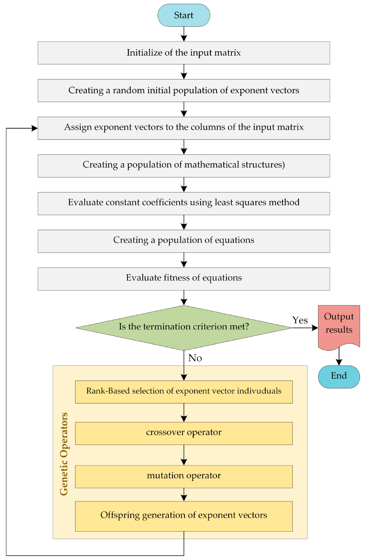
In order to determine the constant coefficients of Equation (11), the least-squares method is used [53]. Additionally, EPR utilizes the GA to find the best mathematical equation based on the suggested exponents [53]. The genetic algorithm (GA) is an evolutionary optimization algorithm inspired by the process of natural selection. This method starts by creating a random primary population from solutions. Each determined parameter represents a person’s chromosome. The fit of each person is also determined based on their performance in the environment. Then, the new population is developed from mutation and crossover operations [57,58]. Figure 1 shows the EPR flowchart.

3. Evaluation of the Model Precision

To assess the precision of the models and compare the models with each other, five statistical indexes were used: the regression coefficient ($R^2$), root mean square error (RMSE), coefficient of determination (CoD), sum of squares error (SSE), and mean errors (AVG). These indexes can be specified via the following relations:

$$R^2={\left[\frac{1}{N}\frac{{{\displaystyle \sum }}_{i=1}^N\left(T_i-\overline{T}\right)\left(O_i-\overline{O}\right)}{{\sigma }_{T }.{\sigma }_O}\right]}^2$$

(12)

$$CoD=1-\frac{{{\displaystyle \sum }}_{i=1}^N{{\displaystyle \sum }}_{N_s}{\left(O_i-T_i\right)}^2}{{{\displaystyle \sum }}_{i=1}^N{\left(T_i-\overline{T}\right)}^2}$$

(13)

$$SSE=\frac{1}{N}{\displaystyle \sum }_{i=1}^N{\left(T_i-O_i\right)}^2$$

(14)

$$RMSE=\sqrt{\frac{1}{N}.{\displaystyle \sum }_{i=1}^N{\left(T_i-O_i\right)}^2}$$

(15)

$$AVG=\frac{{{\displaystyle \sum }}_{i=1}^N \sqrt{{\left(1-T_i/O_i\right)}^2}}{N}$$

(16)

where N is the number of data points, T_i is the vector of the measured values, $O_i$ is the vector of the predicted values, $\overline{T}$ is the mean of the measured values, $\overline{O}$ is the mean of the predicted values, ${\sigma }_{T }$is the SD of the measured values, and ${\sigma }_O$ is the SD of the predicted values.

4. Dataset

4.1. Description of Dataset

The dataset used in this study was taken from the experimental study by Oshtaghi and Mahinroosta (2014) [20], which was extracted in turn from Hasanzadehshooiili et al. [46]. The aim of these experiments was to explore the collapse phenomenon in sandy gravel soils and its influential factors. To this end, a large-scale direct shear test was used with a $30\times 30\times 15$ cm box. First, dry soil with specified relative density was sheared under fixed normal stress until a pre-determined shear stress was achieved. Then, the materials were saturated. After saturation, which was accompanied by collapse settlement, the shear process continued until the rupture stage.

Numerous parameters affect the collapse settlement. Therefore, for a comprehensive study of the collapse behaviour of materials, the effects of all parameters should be taken into account. In line with this, all related parameters were here considered by reviewing related studies. Then, the influential parameters were determined based on their kind. These parameters included sand content (SC), normal stress (${\sigma }_n$), shear stress level (SL), and relative density (Dr). Additionally, collapse settlement (∆H) and coefficient of stress release (CSR) were used as output parameters. It should also be noted that, in this study, the clay content of materials did not considerably change. Furthermore, the primary moisture content was also fixed. Finally, 180 data points were prepared by using a large-scale direct shear test [20].

4.2. Statistical Parameters

For modelling, first, data were randomly divided into training and testing groups, with 70% of data selected as the training set and 30% as the testing set.

Table 1. Statistical features of training data.

Statistical Index	SC (%)	${\mathit{\sigma }}_{\mathit{n} }(\mathbf{kg}/{\mathbf{cm}}^2)$	SL (%)	Dr (%)	CSR	∆H (mm)
Min.	0	1	30	60	0.289	0.11
Max.	100	5	100	85	0.779	2.92
Mean	51.98	3.03	64.72	71.42	0.49	1.08
Median	50	3	62.5	70	0.5	0.94
Standard deviation	41.66	1.39	27.12	10.46	0.11	0.73

and

Table 2. Statistical features of testing data.

Statistical Index	SC (%)	${\mathit{\sigma }}_{\mathit{n} }(\mathbf{kg}/{\mathbf{cm}}^2)$	SL (%)	Dr (%)	CSR	∆H (mm)
Min.	0	1	30	60	0.297	0.12
Max.	100	5	100	85	0.769	2.85
Mean	45.37	2.92	61.48	71.22	0.51	1.18
Median	50	3	62.5	70	0.5	1.03
Standard deviation	39.17	1.47	24.66	9.98	0.1	0.77

show the statistical parameters of the input and output parameters for the training and testing sets, respectively. Figure 2 also presents the frequency and cumulative frequency histograms of all input and output data.

As can be seen, the SC varied in the range from 0 to 100%, ${\sigma }_n$ varied in the range from 1 to 5 kg/cm², SL varied in the range from 30 to 100%, and Dr varied in the range from 60 to 85%. Additionally, the measured collapse settlement varied in the range from 0.11 to 2.92 mm and the CSR varied in the range from 0.289 to 0.779. The wide range of input and outputs parameters confirms the high variety in the samples.

5. Modelling Based on EPR Method

5.1. Developing Prediction Models for ∆H and CSR

The dataset described in Section 4 was employed to develop EPR models. The development of the EPR models was undertaken by assuming the influence of the four variables sand content (SC), normal stress (σ_n), shear stress level (SL), and relative density (Dr) on the collapse settlement (∆H) and coefficient of stress release (CSR). Due to the small changes in the percentage of clay content, this variable was not considered in the modelling, and the initial moisture was also assumed to be constant. The overall procedure for developing the predictive models for ∆H and CSR is depicted in Figure 3.

After normalization and partitioning of data, the modelling process was completed using the EPR method. This process is based on inner functions, such as the exponential, natural logarithm, sinusoidal, tangent hyperbolic, and secant hyperbolic. The EPR-MOGA program, a MATLAB tool, was employed to develop the EPR models. The best model for each of the functions and structures was selected based on the smallest error in the modelling. The structure of EPR model for the prediction of the collapse settlement was developed to be similar to Equation (17) in the secant hyperbolic and natural and exponential logarithms, Equation (18) in the tangent hyperbolic, and Equation (19) in the sinusoidal model. Furthermore, to predict the coefficient of stress release, the structure of EPR model was assumed to be similar to Equation (17) in the secant hyperbolic and exponential models, Equation (18) in tangent hyperbolic and natural logarithm models, and Equation (19) in the sinusoidal model.

$$Y=sum\left(a_i\times X_1\times X_2\times f\left(X_1\right)\times f\left(X_2\right)\right)+a_0$$

(17)

$$Y=sum\left(a_i\times X_1\times X_2\times f\left(X_1\times X_2\right)\right)+a_0$$

(18)

$$Y=\sin \left(sum\left(a_i\times X_1\times X_2\right)+a_0\right)$$

(19)

The other details related to the development of the EPR predictive models are shown in

Table 3. Details of arranged parameters of EPR models for prediction of collapse settlement.

Parameter	Parameter Arrangement
	Sinusoidal	Exponential	Natural Logarithm	Tangent Hyperbolic	Secant Hyperbolic
Exponential range	[−1, −0.5, 0, 0.5, 1]	[−1, −0.5, 0, 0.5, 1]	[−1, −0.5, 0, 0.5, 1]	[−1, −0.5, 0, 0.5, 1]	[−1, −0.5, 0, 0.5, 1]
Number of terms	5	5	5	5	5
Bias value	−0.056354	−0.63544	−0.025247	2.6271	−4.6782
Parameter scale	[0, 1]	[0, 1]	[0, 1]	[0, 1]	[0, 1]

and

Table 4. Details of arranged parameters of EPR models for prediction of coefficient of stress release.

Parameter	Parameter Arrangement
	Sinusoidal	Exponential	Natural Logarithm	Tangent Hyperbolic	Secant Hyperbolic
Exponential range	[−1, −0.5, 0, 0.5, 1]	[−1, −0.5, 0, 0.5, 1]	[−1, −0.5, 0, 0.5, 1]	[−1, −0.5, 0, 0.5, 1]	[−1, −0.5, 0, 0.5, 1]
Number of terms	5	5	5	5	5
Bias value	1.0927	0.28029	0.83969	0.097054	1.2518
Parameter scale	[0, 1]	[0, 1]	[0, 1]	[0, 1]	[0, 1]

.

The representative range shown in the tables determined the linearity or nonlinearity of the model, as well as the direct or reverse dependence between the input variables and output variable. The optimal models for the different functions for predicting collapse settlement are presented in Equations (20)–(24), and those for predicting the coefficient of stress release are shown in Equations (25)–(29).

Secant hyperbolic

$$\begin{gathered} \Delta H=4.3437·\frac{1}{sech{\left(SC\right)}^{0.5}}+0.36122·\frac{1}{sech\left({\sigma }_n\right).sech\left(SL\right)}-0.064019·D{r}^{0.5}.\frac{sech{\left(SC\right)}^{0.5}.sech\left(Dr\right)}{sech\left(SL\right)} \\ -0.46804·SC.\frac{1}{sech\left(SC\right).sech\left({\sigma }_n\right)}+0.68941·SC.{\sigma }_n.sech{\left({\sigma }_n\right)}^{0.5}-4.6782 \end{gathered}$$

(20)

Tangent hyperbolic

$$\begin{gathered} \Delta H=-1.8072·\tanh \left(\frac{1}{SC}\right)-0.8547·\tanh \left(\frac{1}{SL}\right)+0.34027·S{L}^{0.5}.\tanh \left(\frac{SC.{\sigma }_n}{S{L}^{0.5}}\right) \\ -0.1282·SL.\tanh \left(\frac{S{C}^{0.5}.D{r}^{0.5}}{SL}\right)+0.24921·{\sigma }_n.\tanh \left(\frac{1}{SC.{\sigma }_n.S{L}^{0.5}}\right)+2.6271 \end{gathered}$$

(21)

Natural logarithm

$$\begin{gathered} \Delta H=-2.9734·Ln\left(SC+1\right)+0.33875·SL.Ln\left(SL+1\right)+0.24728·{\sigma }_n.Ln{\left({\sigma }_n+1\right)}^{0.5} \\ +0.26894·S{C}^{0.5}.Ln{\left({\sigma }_n+1\right)}^{0.5}+2.4068·SC-0.025247 \end{gathered}$$

(22)

Exponential

$$\begin{gathered} \Delta H=+0.20777·\exp \left(0.5·{\sigma }_n-SL\right)+0.43164·\exp \left(SC\right)-0.028606·D{r}^{0.5}.\exp \left(SL\right)+ \\ 0.12536·S{L}^{0.5}.\exp \left(0.5·{\sigma }_n+SL\right)-0.37924·S{C}^{0.5}.\exp \left(-{\sigma }_n\right)-0.63544 \end{gathered}$$

(23)

Sinusoidal

$$\Delta H=\sin \left(+0.15549·SL+0.2798·{\sigma }_n-0.88635·S{C}^{0.5}+1.3442·SC+0.52595·SC.{\sigma }_n.SL-0.056354\right)$$

(24)

Secant hyperbolic

$$\begin{array}{l}CSR=-0.41461·\frac{sech\left(SC\right).sech{\left(Dr\right)}^{0.5}}{sech\left(SL\right)}-0.43654·S{L}^{0.5}.\frac{sech{\left(SL\right)}^{0.5}}{sech\left(SC\right).sech{\left(Dr\right)}^{0.5}}\\ +0.05815·{\sigma }_n.\frac{sech{\left(Dr\right)}^{0.5}}{sech\left(SC\right).sech\left(SL\right)}-0.29208· S{C}^{0.5}.\frac{1}{sech\left(SC\right)}\\ +0.1766·S{C}^{0.5}.S{L}^{0.5}.\frac{sech{\left(SC\right)}^{0.5}}{sech{\left({\sigma }_n\right)}^{0.5}.sech\left(Dr\right)}+1.2518 \end{array}$$

(25)

Tangent hyperbolic

$$\begin{gathered} CSR=0.59952·\tanh \left(\frac{1}{SC}\right)+0.19982·\tanh \left(\frac{SL}{SC}\right)+0.070066·\tanh \left(\frac{{\sigma }_n{}^{0.5}.SL.D{r}^{0.5}}{SC}\right)-0.88554·S{L}^{0.5} \\ +0.1074·{\sigma }_n.\tanh \left({\sigma }_n{}^{0.5}\right)+0.097054 \end{gathered}$$

(26)

Natural logarithm

$$CSR=0.039507·D{r}^{0.5}-0.47·S{L}^{0.5}+0.0019608·SL.Ln\left(\frac{SC.{\sigma }_n{}^{0.5}}{S{L}^{0.5}}\right)+0.084114·{\sigma }_n-0.33821·SC+0.83969$$

(27)

Exponential

$$\begin{gathered} CSR=0.52381·\exp \left(-SC\right)+0.034596·\exp \left(SC+0.5·{\sigma }_n+SL\right)-0.38976·S{L}^{0.5}.\exp \left(-SC+0.5·SL\right)+ \\ 0.17439·{\sigma }_n{}^{0.5}.D{r}^{0.5}.\exp \left(-SC-SL-0.5·Dr\right)-0.18081·SC.S{L}^{0.5}.\exp \left(SC\right)+0.28029 \end{gathered}$$

(28)

Sinusoidal

$$\begin{gathered} CSR=sin\left(-0.8422·S{L}^{0.5}+0.12979·{\sigma }_n-0.53025·S{C}^{0.5}+0.93854·S{C}^{0.5}.S{L}^{0.5}-0.65962·SC.S{L}^{0.5}+ \\ 1.0927\right) \end{gathered}$$

(29)

In the above equations, we have:

SC: the normalized value of the sand content in percentage;

${\sigma }_n$: the normalized value of the normal stress in kg/cm²;

SL: the normalized value of shear stress as a percentage;

Dr: the normalized value of the relative density as a percentage;

∆H: the normalized value of the collapse settlement in mm;

CSR: the normalized value of the coefficient of stress release.

The normalized value of each parameter was calculated as follows:

$$\mathrm{x}\prime =\frac{\mathrm{x}-{\mathrm{x}}_{\min }}{{\mathrm{x}}_{\max }-{\mathrm{x}}_{\min }}$$

(30)

in which:

$x$: the quantity value at the real scale;

$x\prime$: the normalized value of the quantity;

$x_{min}$: the smallest value of the quantity;

$x_{max}$: the greatest value of the quantity;

Table 1 shows the minimum and maximum values of the parameters.

5.2. Evaluating the Model Performance

In

Table 5. Precision and performance of the models for ∆H prediction (training data).

Models	COD	AVG	RMSE	SSE	R2
Secant hyperbolic	0.9784	0.125	0.01	0.011	0.9781
Tangent hyperbolic	0.9743	0.144	0.011	0.013	0.9744
Natural logarithm	0.9625	0.16	0.014	0.02	0.9626
Exponential	0.9759	0.116	0.01	0.012	0.9759
Sinusoidal	0.9568	0.182	0.013	0.023	0.9571

,

Table 6. Precision and performance of the models for ∆H prediction (testing data).

Models	COD	AVG	RMSE	SSE	R2
Secant hyperbolic	0.9728	0.111	0.014	0.015	0.9732
Tangent hyperbolic	0.9733	0.142	0.016	0.021	0.9634
Natural logarithm	0.9667	0.134	0.02	0.019	0.9668
Exponential	0.9746	0.101	0.013	0.014	0.9759
Sinusoidal	0.9374	0.204	0.018	0.036	0.938

,

Table 7. Precision and performance of the models for ∆H prediction (all data).

Models	COD	AVG	RMSE	SSE	R2
Secant hyperbolic	0.9785	0.125	0.015	0.012	0.9768
Tangent hyperbolic	0.9746	0.142	0.017	0.014	0.971
Natural logarithm	0.9615	0.16	0.019	0.021	0.9641
Exponential	0.9758	0.116	0.014	0.013	0.9757
Sinusoidal	0.9569	0.182	0.019	0.023	0.9512

,

Table 8. Precision and performance of models for CSR prediction (training data).

Models	COD	AVG	RMSE	SSE	R2
Secant hyperbolic	0.9812	0.025	0.01	0.0002	0.9812
Tangent hyperbolic	0.9781	0.03	0.011	0.0002	0.9781
Natural logarithm	0.9706	0.036	0.014	0.0003	0.9706
Exponential	0.9833	0.012	0.01	0.0002	0.9833
Sinus	0.9687	0.015	0.013	0.0004	0.9694

,

Table 9. Precision and performance of models for CSR prediction (testing data).

Models	COD	AVG	RMSE	SSE	R2
Secant hyperbolic	0.98	0.023	0.014	0.0002	0.9803
Tangent hyperbolic	0.9722	0.028	0.016	0.0002	0.9733
Natural logarithm	0.9593	0.035	0.02	0.0004	0.9607
Exponential	0.9817	0.022	0.013	0.0001	0.982
Sinus	0.9655	0.027	0.018	0.0003	0.9663

and

Table 10. Precision and performance of models for CSR prediction (all data).

Models	COD	AVG	RMSE	SSE	R2
Secant hyperbolic	0.9812	0.025	0.015	0.0003	0.9811
Tangent hyperbolic	0.978	0.03	0.017	0.0003	0.9769
Natural logarithm	0.9709	0.036	0.019	0.0004	0.9682
Exponential	0.9832	0.025	0.014	0.0002	0.9833
Sinusoidal	0.9685	0.034	0.019	0.0004	0.9687

, the performance parameters of the models for training, testing, and total data are presented. The basis for calculating these parameters was the relations mentioned in Section 3. As is evident, all the models performed desirably in predicting the collapse settlement and coefficient of stress release.

When comparing the models with one another to select the best one, as well as in comparing the performance parameters, simplicity is important. The simplicity and complexity of a model is typically determined based on the exponential coefficients, the number of algebraic expressions, and direct or indirect relation between input and output parameters.

Figure 4, Figure 5, Figure 6, Figure 7 and Figure 8 represent the ability of each developed model by comparing the measured and predicted collapse settlement based on the training and testing sets. Additionally, the error range of 20% is shown. Examining the exponential model, which was already selected as the best model (Figure 7), it can be seen that the R² values for training and testing data were 0.9759 and 0.9759, respectively, and the RMSE values were 0.010 and 0.013, respectively, which in turn indicate the suitable precision of the model.

Figure 9, Figure 10, Figure 11, Figure 12 and Figure 13 show the ability of each of the developed models by comparing the measured and predicted coefficients of stress release based on the training and testing data. Similarly, the error range of 20% is shown. It can be clearly seen that the R² values for training and testing data were 0.9833 and 0.9820, respectively, and the RMSE values were 0.010 and 0.013, respectively, which in turn indicate the suitable precision of the model.

5.3. Comparing the Developed Model with Other Models

In order to evaluate the ability of the EPR, the results obtained were compared and contrasted with those of other models. To this end, the results of the ANN model developed by Hasanzadehshooiili et al. [46] and those of the MGGP model developed by Soleimani et al. [47] were used.

Table 11. Comparing the R² values of the EPR model with other models.

Models	EPR		ANN [46]		MGGP [47]
Dataset	Training	Testing	Training	Testing	Training	Testing
∆H	0.9759	0.9759	0.9828	0.9830	0.9780	0.9580
CSR	0.9833	0.9820	0.9806	0.9810	0.9610	0.9820

compares the R² results from the EPR with those of the ANN and MGGP.

As can be, the EPR model predicted the coefficient of stress release (CSR) with higher precision compared to the ANN model, while the ANN model showed higher precision compared to the EPR model in predicting the collapse settlement (∆H) of sandy gravel soil. However, using the EPR model over the ANN model is preferred due to its simplicity and transparency. In fact, EPR-based models can easily be implemented with manual calculations. As shown in Table 11, the EPR model was more capable compared to the MGGP model in predicting the ∆H and CSR of sandy gravel soil. Further, when predicting ∆H with the MGGP model, the R² of the testing data was lower than that for the training data, which indicates the over-fitting of the MGGP model in this case. Further, regarding the prediction of CSR using the MGGP model, the R² of the training data was lower than for the testing data, which could have been due to the improper partitioning of the data or the under-fitting of the developed MGGP model. Compared to the MGGP model, the EPR models presented in this research gave almost the same values for the coefficient of determination (R²) for the training and the testing data, which indicates that the EPR models did not over-fit.

6. Sensitivity Analysis

In this study, the cosine amplitude method (CAM) was used in a sensitivity analysis to determine the degree of importance of the input parameters in influencing the collapse settlement and coefficient of stress release parameters of sandy gravel soil. The degree of importance can be estimated through Equation (31):

$$R_i=\frac{{{\displaystyle \sum }}_{j=1}^n{x}_{ij}.y_j}{\sqrt{{{\displaystyle \sum }}_{j=1}^n{x}_{ij}{}^2.{{\displaystyle \sum }}_{j=1}^n{y}_j{}^2}}$$

(31)

where x_ij is the ith variable for jth data point, and y_j is the dependent variable for the jth data point. When R_i is closer to 1, it indicates higher importance for the input parameter in estimating the output parameter, and if R_i is zero, there is no correlation.

Figure 14 and Figure 15 present the importance degree of importance of the input variables based on the measured and predicted values for the collapse settlement and coefficient of stress release, respectively. As the figures show, SC and Dr were the most and least important parameters for predicting collapse settlement. In contrast, Dr and Sc were the most and least important parameters for predicting the coefficient of stress release. Moreover, the differences in R_i based on the predicted and the measured values of collapse settlement for the SC, ${\mathsf{\sigma }}_n,$ SL, and Dr variables were 0.57%, 0.05%, 0.05%, and 0.05%, respectively. These values for the coefficient of stress release were 0.01%, 0.13%, 0.02%, and 0.02%, respectively. The small percentages for these differences, in turn, indicate the high precision of the EPR models in predicting the collapse settlement and coefficient of stress release.

7. Parametric Study

Cost and time restrictions, as well as limited access to applicable equipment, are typically the main problems in laboratory studies. In most cases, examining the effects of each input variable on the output variables requires preparing several samples, which is costly and time consuming. One merit of modelling is that developed models can be used for parametric studies and evaluation of the impact of each input variable on the model output.

As was already noted, in this study, the input parameters were SC, ${\mathsf{\sigma }}_n$, Dr, and SL. This study made use of the optimal EPR model to examine the interation impact of SC and Dr, Dr and ${\mathsf{\sigma }}_n,$ Dr and SL, and SL and ${\mathsf{\sigma }}_n$ on the collapse settlement and coefficient of stress release. To this end, the desired variable altered between its minimum and maximum values and other variables were considered equal to the mean value. Then, the collapse settlement and coefficient of stress release were determined via EPR. The pertinent results are shown in Figure 16 and Figure 17.

The interaction of ${\mathsf{\sigma }}_n$ and SL indicates that increasing SL led to an increase in the collapse settlement and a reduction in the coefficient of stress release. Additionally, an increase in ${\mathsf{\sigma }}_n$ led to an increase in both the collapse settlement and coefficient of stress release. Furthermore, the interaction of SC and Dr indicated the high impact of SC in increasing the collapse settlement and decreasing the coefficient of stress release. The trivial effect of Dr in increasing the coefficient of stress release and decreasing the collapse settlement is obvious. The interaction of Dr and ${\mathsf{\sigma }}_n$ also revealed that an increase in ${\mathsf{\sigma }}_n$ resulted in increases in both the collapse settlement and the coefficient of stress release. Increases in Dr also increased the coefficient of stress release and decreased collapse settlement. The interaction of SL and Dr implied a remarkable effect of SL on increasing the collapse settlement and coefficient of stress release. Finally, the changes related to Dr implied that an increase in Dr resulted in increasing the coefficient of stress release and decreasing the collapse settlement.

Table 12. Comparing the influence of input parameter changes on collapse settlement and coefficient of stress release.

Input Parameters	Input Parameter Changes	Collapse Settlement Changes			Stress Release Changes
		Hasanzadehshooiili et al. [46]	Soleimani et al. [47]	This Study	Hasanzadehshooiili et al. [46]	Soleimani et al. [47]	This Study
${\mathsf{\sigma }}_n$	Increase	Increase	Increase	Increase	Increase	Increase	Increase
SC	Increase	Increase	Increase	Increase	Decrease	Decrease	Decrease
SL	Increase	Increase	Increase	Increase	Decrease	Decrease	Decrease
Dr	Increase	Decrease	Decrease	Decrease	Increase	Increase	Increase

presents a comparison of the parametric study results for the present study model and the models by Hasanzadehshooiili et al. [46] and Soleimani et al. [47].

Table 12 reveals that the effects of the input variables on the collapse settlement and coefficient of stress release in the EPR model had a similar trend to those of Hasanzadehshooiili et al. [46] and Soleimani et al. [47]. This, in fact, indicates the precision of the developed model.

8. Conclusions

In this study, the collapse settlement and coefficient of stress release of sandy gravel soil were examined. To develop the prediction model, a dataset consisting of 180 samples from a large-scale direct shear test was employed. Using sand content (SC), normal stress (${\sigma }_n$), shear stress level (SL), and relative density (Dr) variables, the developed models could predict the collapse settlement and the coefficient of stress release. The findings of the present study can be summarized as follows:

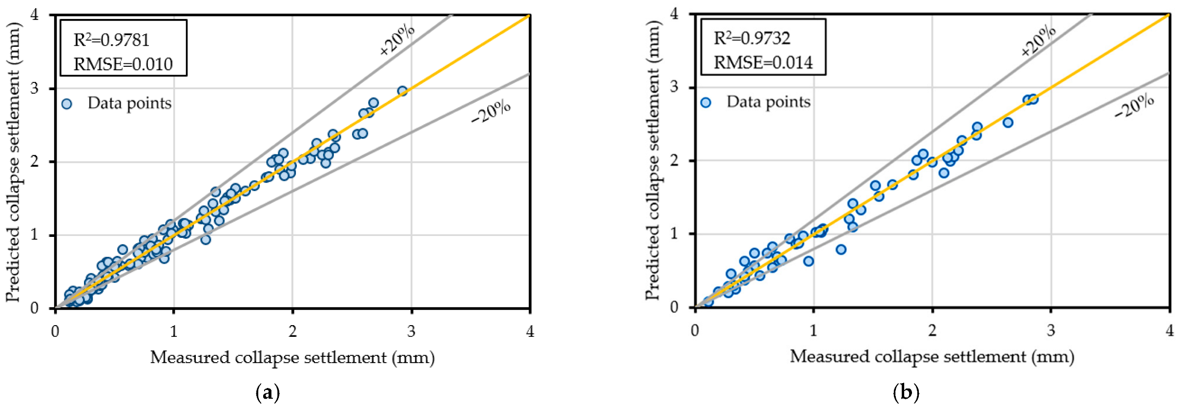
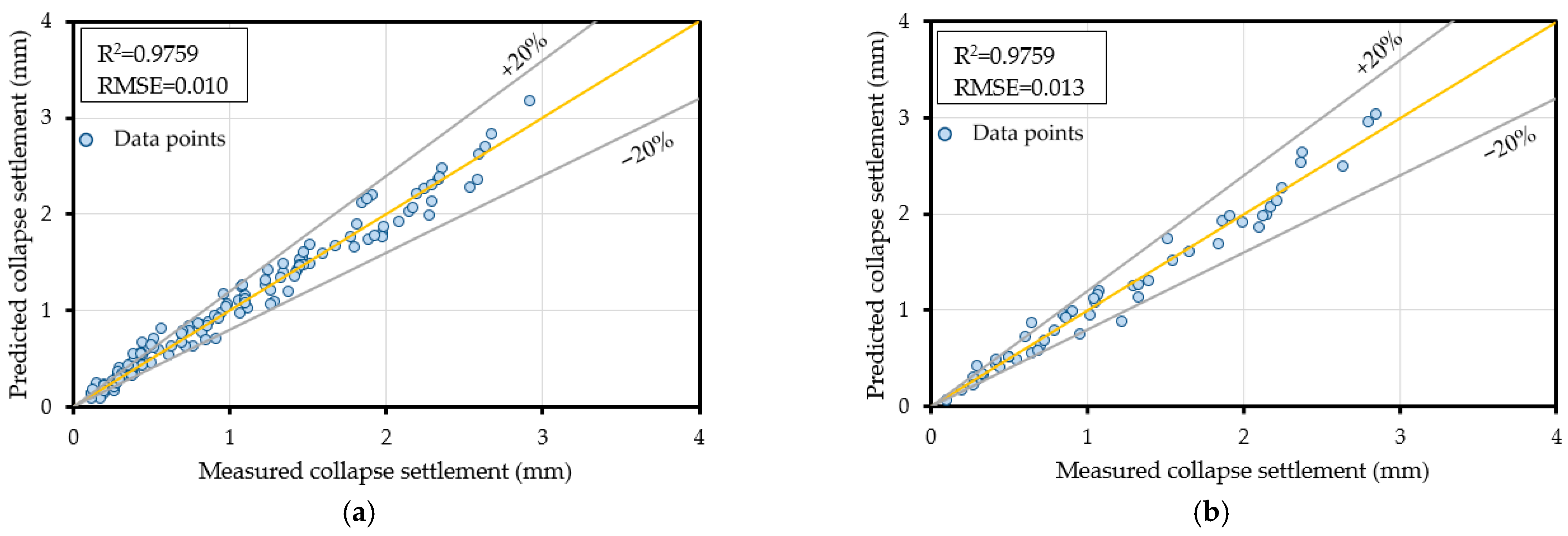
(1) EPR models developed with an exponential function were selected as the optimal models. According to the R² coefficient, the levels of precision of the model in predicting collapse settlement using training, testing, and all data were 0.9759, 0.9759, and 0.9759, respectively, and the precision levels in predicting the coefficient of stress release were 0.9833, 0.9820, and 0.9833, respectively;

(2) The EPR models showed superior performance in predicting the collapse settlement and coefficient of stress release compared to the MGGP model. Additionally, the ANN model showed higher accuracy than the EPR model in predicting collapse settlement. However, the EPR model could predict the coefficient of stress release more precisely compared to the ANN model;

(3) The results of the sensitivity analysis revealed that the SC was the most important and Dr the least important parameter in predicting the collapse settlement. Furthermore, the Dr and SC were found to be the most and least important parameters, respectively, in predicting the coefficient of stress release;

(4) The results of the parametric study confirmed that increases in the SL and SC led to an increase in collapse settlement and a decrease in the coefficient of stress release. Additionally, increasing σ_n caused both collapse settlement and coefficient of stress release to increase. Finally, increases in the Dr variable reduced the collapse settlement and increased the coefficient of stress release;

(5) To continue this research and achieve higher accuracy in predicting the collapse settlement and coefficient of stress release, other machine learning methods could be used.