Dynamic Characteristics Analysis of a Rigid Body System with Spatial Multi-Point Supports

Abstract

This paper presents the dynamic characteristics analysis of a rigid body system with spatial multi-point elastic supports, as well as the sensitivity analysis of support parameters. A rigid object is characterized by six degrees-of-freedom (DOFs) motions and considering the spatial location vector decomposition of elastic supports, a rigid body system dynamic model with spatial multi-point elastic supports is derived via the Lagrangian energy method. The system modal frequencies are calculated, and to be verified by finite element modal analysis results. Next, based on the above-mentioned model, system modal frequencies are obtained under different support locations, where the support stiffness components are different. Interpolate the stiffness components corresponding to each support location, calculate system modal frequencies, and the response surface model (RSM) for system modal frequencies is established. Further, based on the RSM modal analysis results, the allowable support location for the system modal insensitive area can be obtained. At last, a lubricating oil-tank system with four supports is taken as an example, and the effects of support spatial locations and stiffness components on the system inherent characteristics are discussed. This present work can provide a basis for the dynamic design of the spatial location and stiffness for this type of installation structures.

1. Introduction

Some parts of the devices equipped in the industry engineering applications such as aerospace, energy and power, vehicle engineering, and robotics field have the typical characteristics of a rigid body system with spatial multi-point elastic supports, and there are complex rigid body motions [1,2,3]. The dynamic characteristics of a rigid body system with spatial multi-point elastic supports are complex, and it is particularly prone to vibration problems such as close frequency, repetitive frequency, and coupled vibration, which will cause vibration or even resonance under external excitation. For example, the lubricating oil-tank component of the aero-engine external device is fixed on the casing through spatial multi-point anchored supporting structure at different locations, and it is a typical large-scale rigid structure with spatial multi-point elastic supports. The lubricating oil-tank system with multi-point elastic supports has the characteristics of large mass, inconsistent support rigidity, and complex modal characteristics, and it is prone to strong vibration or even damage under areo-engine complex vibration excitation. In the design process of the aero-engine lubricating oil-tank and installation structure, it is, therefore, of great need to carry out reasonable dynamic analysis of the rigid body system with spatial multi-point elastic supports. In fact, the dynamic analysis research on a rigid body system with spatial multi-point elastic supports is extensive, and it has been highly valued in many fields recently.

At present, few studies on the dynamics of a lubrication oil tank-mounting structure system with spatial multi-point elastic supports have been documented, and related studies mainly involve automotive powertrain multi-point mounting system, marine power plant and its vibration isolation structure, and aircraft engine nacelle suspension. The related research work is reviewed as follows.

Many achievements have been made in the research on automobile powertrain system dynamics. The core idea of dynamics and optimization design of automobile engine powertrain and its mounting system is to realize the reasonable distribution of powertrain modal frequency and the modal decoupling of the mounting system under excitation, to reduce the vibration transmission rate between the powertrain and the frame, etc. [4,5,6]. Only rigid-body modes of the powertrain are considered, the torque roll axis (TRA) decoupling dynamics equation was established by Jeong and Singh [7], and the spatial multi-point mounting schemes of an automotive engine gearbox system with oscillating torques excitation was obtained. Park and Singh [8] took mount rate ratios, mount locations, and orientation angles as key design parameters to investigate the modal characteristics of the multi-point rigid body system and its TRA decoupling problem. Tao et al. [9] established a dynamic model of the engine mounting system and took the mounting stiffness coefficient and orientations of individual mount as design parameters to optimize the support stiffness value obtained via the modal sensitivity method. Yu et al. [10] demonstrated that the performance of the whole engine mounting system not only depended on the performance of individual mounts, but the multi-point supports of the whole system as well, and it is of need to further consider the nonlinear characteristics of the supports.

The high-power diesel engine-generator set for locomotives or ships is typically a rigid body system with multi-point supports, and it has the characteristics of multi-point elastic supports in space, multiple source excitation, wide frequency domain, complex system dynamics, and is prone to coupled vibrations. In the research on vibration isolation of diesel engine systems of high/medium power levels, some work on the analysis of the arrangement of vibration isolators and the influence of variation of stiffness and damp has been carried out. Zhang et al. [11] established a general dynamics model to describe the system dynamics of high-power engines with different numbers of mounts. Lee et al. [12] established a six-degrees-of-freedom rigid body dynamics model for marine diesel generator sets and conducted an evaluation study on the vibration transmitted from the support to the engine body. With improvement of vibration and noise reduction requirements, complex two-stage vibration isolation systems, and large float raft vibration isolation systems that can carry dozens of power equipment have gradually been developed and applied [13,14,15]. Hu et al. [16] studied the transfer function curve of the two-stage vibration isolation system with different stiffness ratios, and the vibration transfer energy can be reduced when the stiffness ratio of the upper and lower isolators increased as much as possible. Lv et al. [17] endured a multi-parameter optimization method for the natural frequency of the float raft vibration isolation system, where the natural frequency of the vibration isolation system could be limited to a narrow range by optimizing the stiffness of the raft body and the stiffness of the sub-raft connecting rod, to achieve the best vibration isolation effect.

While people were studying the theory and engineering application of two-stage vibration isolation systems, the semi-active and active control of two-stage vibration isolation devices has also received extensive attention, and the main idea is to control the stiffness and to damp the vibration isolation system in real-time through some means to achieve a good vibration isolation effect [18,19,20]. Foumani et al. [21] employed global optimization technology to adjust adaptive hydraulic mount design parameters (mount flexibility, mount inertia parameters, etc.) for tuning an adaptive mount to different road and engine conditions, in order to achieve vibration isolation under low and high frequency excitations.

In addition to the above research on the dynamic characteristics of the multi-support structure system of the power plant for automobiles, locomotives, ships, and in the aviation field, researchers have also studied the dynamic characteristics of the multi-support engine nacelle mounting system, mainly regarding the dynamic coupling characteristics of the engine and the suspension inside the nacelle [22,23].

Few studies on the dynamics of aeroengine lubrication oil tank-mounting structure system have been documented, and studies on the influence of mounting structure (mount number, location, and stiffness, etc.) on aeroengine lubrication oil tank system have not been documented. Li [24] built the fluid-structure interaction model by MSC/Dytran while analysing the influence factor of oil tank sloshing and analysed the structure dynamics by Msc/Nastran. Baeten [25] proposed a three-dimensional, time accurate particle-cluster approach to predict highly dynamic airborne tank fuel sloshing and impact effects, as well as analyzed the dynamic behaviour of fuel inside a more complex geometry by simulating liquid sloshing in a toroidal tank. The results of this showed that fuel impact forces have a significant contribution to the pitch characteristics of external fuel tank. Wang et al. [26] proposed a topology optimization method that considered the local stiffness of the mounting structure of the oil tank assembly, which improved the overall stiffness of the support, while considering the local stiffness. Through this method, the stiffness distribution of the bracket became more reasonable.

In summary, there are few studies on the dynamics of rigid body systems with spatial multi-point elastic supports, and there is a gap in the dynamics research of the lubrication oil tank-mounting structure system. Therefore, this paper takes the aero-engine lubrication oil tank-mounting structure system as a representative object to study the dynamic characteristics of a rigid body system with spatial multi-point elastic supports. Firstly, based on the energy method, the kinetic equation of a rigid body system with multiple elastic supports is derived. Then, the effects of spatial location components and stiffness components of each support are all discussed further. Finally, some new results for the rigid body structural system with multiple elastic supports are illustrated, and some suggestions are given from an engineering point of view to guide the dynamic design of the rigid structural system.

2. Dynamic Model of a Rigid Body System with Multi-Point Elastic Supports

2.1. Simplified Model Description

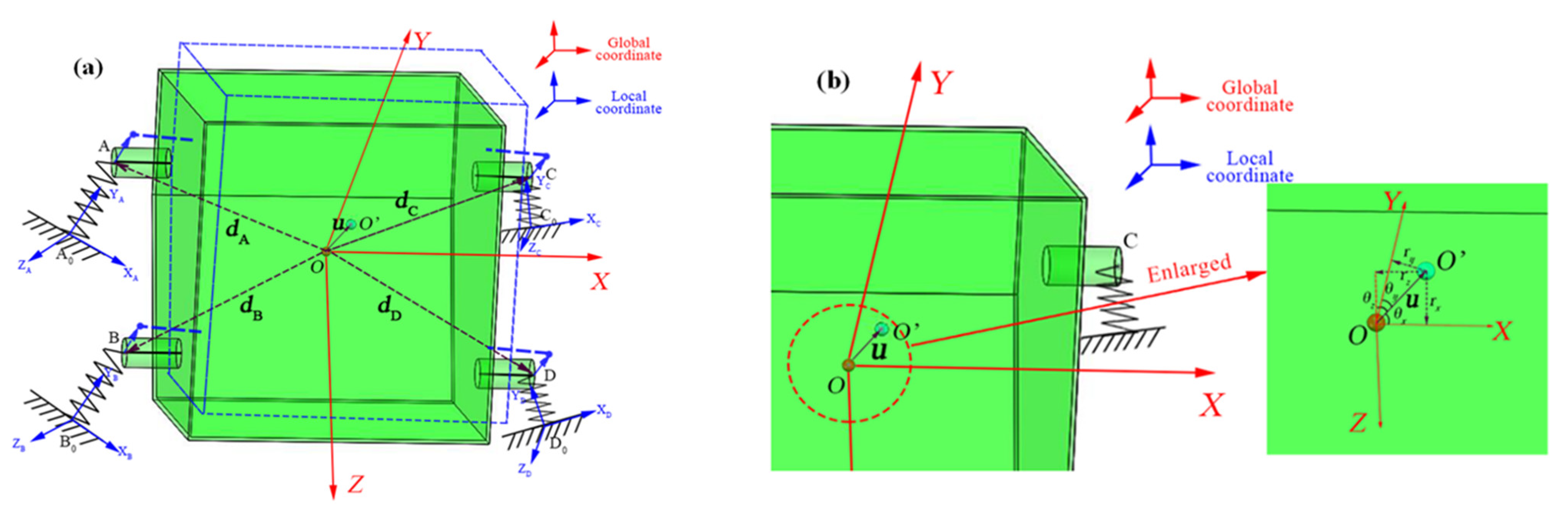
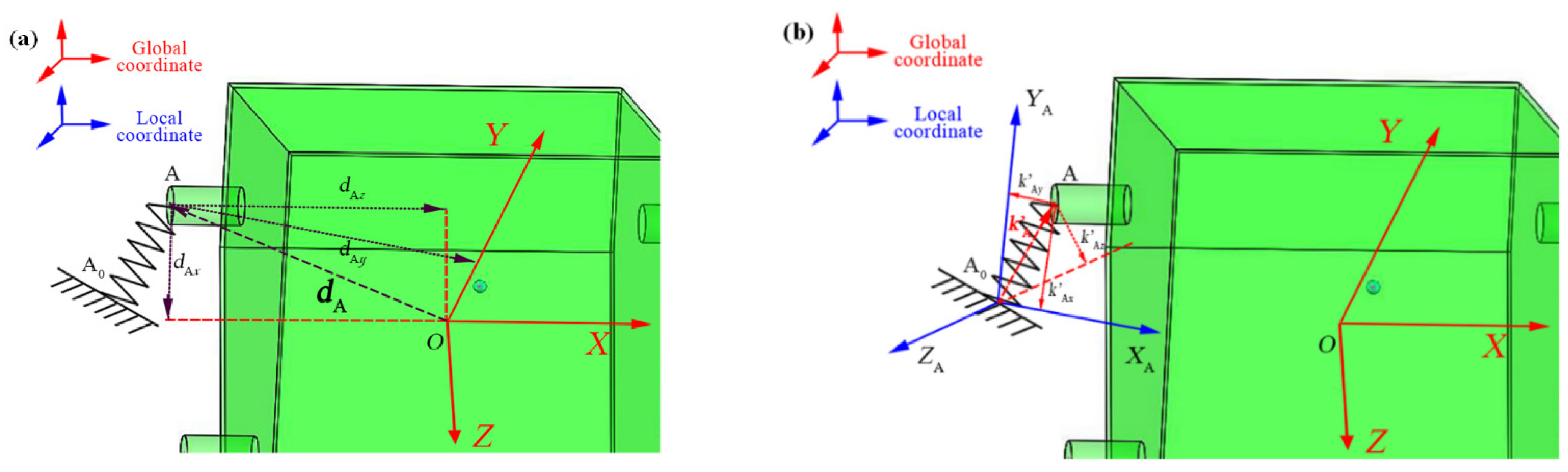
A simplified rigid body system with spatial multi-point elastic supports is illustrated in Figure 1. The rigid body structure is with the mass (m), the moment of inertia tensor is $\mathbf{J}={(J_x,J_y,J_z)}^{\mathrm{T}}$. A global coordinate system O-XYZ with the origin (O) located at the center of the mass is adopted. The rigid body displacement $\mathbf{u}=(\mathbf{r},\mathsf{\theta })$ is composed to the displacement $\mathbf{r}={(r_x,r_y,r_z)}^{\mathrm{T}}$ and the rotation $\theta ={({\theta }_x,{\theta }_y,{\theta }_z)}^{\mathrm{T}}$ around the center of mass. The rigid body is mounted by N supports, and the distance vector from each support to the center of mass is ${\mathbf{d}}_n=(d_{nx},d_{ny},d_{nz})$. Each support provides a three-dimensional elastic constraint ${\mathbf{k}}_n=diag(k_{nx},k_{ny},k_{nz})$. A local coordinate system is built located on each support to facilitate subsequent stiffness component calculations for each support. Take the top-left support for example, and the local coordinate system A₀-X_AY_AZ_A is built, where ${k^{\prime }}_{Ax}$, ${k^{\prime }}_{Ay}$, and ${k^{\prime }}_{Az}$, respectively represent top-left support stiffness components along three directions of the local coordinate axes x_A, y_A, and z_A, as shown in Figure 2.

2.2. Derivation of Frequency Equation Based on Energy Equations

The overall displacement of the simplified rigid body is composed of the displacement $\mathbf{r}={(r_x,r_y,r_z)}^{\mathrm{T}}$ and the rotation $\theta ={({\theta }_x,{\theta }_y,{\theta }_z)}^{\mathrm{T}}$ around the center of mass. According to the overall displacement of the rigid body, the vibration displacement of the n-th support can be obtained by:

$${\mathbf{r}}_{\mathrm{n}}=\mathbf{r}+\mathsf{\theta }\times {\mathbf{d}}_{\mathrm{n}}=(r_x,r_y,r_z)+({\theta }_x,{\theta }_y,{\theta }_z)\times (d_{nx},d_{ny},d_{nz})$$

(1)

where r_x, r_y, and r_z represent the displacements of the center of mass in x, y, and z directions under the global coordinate system, accordingly. θ_x, θ_y, and θ_z represent the rotation angles of the center of mass x, y, and z directions under the global coordinate system, respectively. d_nx, d_ny, and d_nz denote distances in x, y, and z directions from each support to the center of mass.

The vibrational kinetic energy of the rigid body can be calculated as follows:

$$T=\frac{1}{2}\dot{\mathbf{r}}·\mathbf{m}·\dot{\mathbf{r}}+\frac{1}{2}\dot{\mathsf{\theta }}·\mathbf{J}·\dot{\mathsf{\theta }}$$

(2)

The elastic potential energy provided by supports can be calculated as follows:

$$V=\frac{1}{2}{\displaystyle \sum _{\mathrm{n}=1}^{\mathrm{N}}{\mathbf{r}}_{\mathrm{n}}\times {\mathbf{k}}_{\mathrm{n}}\times {\mathbf{r}}_{\mathrm{n}}}$$

(3)

By substituting Equation (1) into Equation (3), the elastic potential energy of the rigid body can be written as:

$$V=\frac{1}{2}{\displaystyle \sum _{\mathrm{n}=1}^{\mathrm{N}}(\mathbf{r}+\mathsf{\theta }\times {\mathbf{d}}_n)\cdot {\mathbf{k}}_{\mathrm{n}}\cdot (\mathbf{r}+\mathsf{\theta }\times {\mathbf{d}}_n)}$$

(4)

Expand Equations (2) and (4), and the vibrational kinetic energy T and elastic potential energy V of the rigid body can be written as:

$$T=\frac{1}{2}m\stackrel{}{{\dot{r}}_x{}^2}+\frac{1}{2}m\stackrel{}{{\dot{r}}_y{}^2}+\frac{1}{2}m\stackrel{}{{\dot{r}}_z{}^2}+\frac{1}{2}{J}_x\stackrel{}{{\dot{\theta }}_x{}^2}+\frac{1}{2}{J}_y\stackrel{}{{\dot{\theta }}_y{}^2}+\frac{1}{2}{J}_z\stackrel{}{{\dot{\theta }}_z{}^2}$$

(5)

where J_x, J_y, and J_z represent the moment of inertia components of the rigid body around in x, y, and z directions, under the global coordinate system, respectively.

$$\begin{array}{cc}V& ={\displaystyle \sum _{n=1}^{\mathrm{N}}\frac{1}{2}}{k}_{nx}{\left(r_x+d_{nz}\cdot {\theta }_y-d_{ny}\cdot {\theta }_z\right)}^2+{\displaystyle \sum _{n=1}^{\mathrm{N}}\frac{1}{2}}{k}_{ny}{\left(r_y-d_{nz}\cdot {\theta }_x+d_{nx}\cdot {\theta }_z\right)}^2+\\ & {\displaystyle \sum _{n=1}^{\mathrm{N}}\frac{1}{2}}{k}_{nz}{\left(r_z+d_{ny}\cdot {\theta }_x-d_{nx}\cdot {\theta }_y\right)}^2\hfill \end{array}$$

(6)

where k_nx, k_ny, and k_nz denote the stiffness component of each support in x, y, and z directions under the global coordinate system.

Substitute the above energy expressions into the Lagrange equations L = T − V, and minimizing L yields the following eigenvalue equations:

$$(\mathbf{K}-{\omega }^2\mathbf{M})\mathbf{u}=\mathbf{0}$$

(7)

where K is the stiffness matrix, M is the mass matrix, and u is the displacement matrix.

$$\mathbf{u}=(r_x,r_y,r_z,{\theta }_x,{\theta }_y,{{\theta }_z)}^{\mathrm{T}}$$

(8)

$$\mathbf{M}=\left(\begin{array}{cccccc}m& & & & & \\ & m& & & & \\ & & m& & & \\ & & & J_x& & \\ & & & & J_y& \\ & & & & & J_x\end{array}\right)$$

(9)

$$\mathbf{K}=\left(\begin{array}{cccccc}{\displaystyle \sum _{n=1}^N{k}_{nx}}& 0& 0& 0& {\displaystyle \sum _{n=1}^N{k}_{nx}{d}_{nz}}& -{\displaystyle \sum _{n=1}^N{k}_{nx}{d}_{ny}}\\ 0& {\displaystyle \sum _{n=1}^N{k}_{ny}}& 0& -{\displaystyle \sum _{n=1}^N{k}_{ny}{d}_{nz}}& 0& {\displaystyle \sum _{n=1}^N{k}_{ny}{d}_{nx}}\\ 0& 0& {\displaystyle \sum _{n=1}^N{k}_{nz}}& {\displaystyle \sum _{n=1}^N{k}_{nz}{d}_{ny}}& -{\displaystyle \sum _{n=1}^N{k}_{nz}{d}_{nx}}& 0\\ 0& -{\displaystyle \sum _{n=1}^N{k}_{ny}{d}_{nz}}& {\displaystyle \sum _{n=1}^N{k}_{nz}{d}_{ny}}& {\displaystyle \sum _{n=1}^N\left(k_{ny}{d}_{nz}^2+k_{nz}{d}_{ny}^2\right)}& -{\displaystyle \sum _{n=1}^N{k}_{nz}{d}_{nx}{d}_{ny}}& -{\displaystyle \sum _{n=1}^N{k}_{ny}{d}_{nx}{d}_{nz}}\\ {\displaystyle \sum _{n=1}^N{k}_{nx}{d}_{nz}}& 0& -{\displaystyle \sum _{n=1}^N{k}_{nz}{d}_{nx}}& -{\displaystyle \sum _{n=1}^N{k}_{nz}{d}_{nx}{d}_{ny}}& {\displaystyle \sum _{n=1}^N\left(k_{nx}{d}_{nz}^2+k_{nz}{d}_{nx}^2\right)}& -{\displaystyle \sum _{n=1}^N{k}_{nx}{d}_{ny}{d}_{nz}}\\ -{\displaystyle \sum _{n=1}^N{k}_{nx}{d}_{ny}}& {\displaystyle \sum _{n=1}^N{k}_{ny}{d}_{nx}}& 0& -{\displaystyle \sum _{n=1}^N{k}_{ny}{d}_{nx}{d}_{nz}}& -{\displaystyle \sum _{n=1}^N{k}_{nx}{d}_{ny}{d}_{nz}}& {\displaystyle \sum _{n=1}^N\left(k_{ny}{d}_{nx}^2+k_{nx}{d}_{ny}^2\right)}\end{array}\right)$$

(10)

The natural frequencies of a rigid body system with spatial multi-point elastic support can be obtained by solving the eigenvalue problem of Equation (7).

3. Structural Parameters Determination and Model Verification

First, perform static analysis on each support to obtain the stiffness component of them in the local coordinate system. Meanwhile, the stiffness component of each support in the global coordinate system is obtained through coordinate transformation. Next, based on the analytical model established above, the first six natural frequencies of a rigid body system with four supports are calculated. At last, finite element analysis is conducted on the simplified rigid body system with four supports, and the rationality of the established analytical model is verified by comparing the modal analysis results.

3.1. The Main Parameters of the Structural System

3.1.1. Determination of Rigid Body Structure Parameters

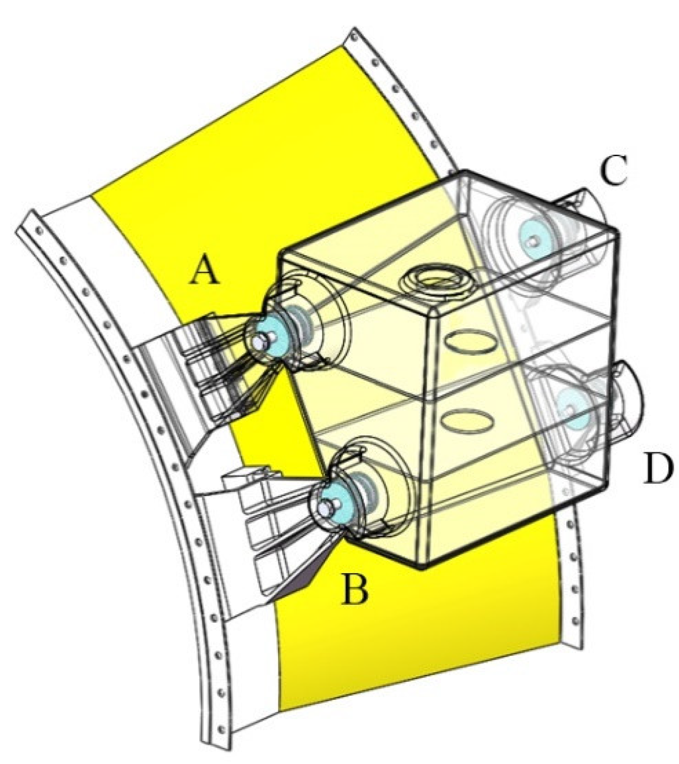
A simplified model of a rigid body object with multi-point supports is shown in Figure 3. This component is a typical rigid body system with four supports, and is mainly assembled by the casing, installation structure components, structural body, and other parts. Both the structural body and the installation structure components are made of #45 steel. Letters A to D indicate the top-left support, bottom-left support, top-right support, and bottom-right support of the rigid body, respectively.

Extract of the main structural parameters of the rigid body, according to the global coordinate system O-XYZ, as shown in

Table 1. Inertial parameters of the simplified rigid body.

Property	Symbol	Value	Unit
Mass	m	11.76	kg
Moment of inertia about the x-axis	Jx	264,706	kg·mm2
Moment of inertia about the y-axis	Jy	309,764	kg·mm2
Moment of inertia about the z-axis	Jz	255,256	kg·mm2

and

Table 2. Definition of each support position in the global coordinate system.

Location (mm)	Mount #
	A	B	C	D
dx	−211	−211	211	211
dy	−13.08	−7.54	13.15	−24.15
dz	−96.38	108.3	−77.66	120.3

, where the x-axis is along the axial direction of the casing, the y-axis is along the normal direction of the casing, and z-axis is along the tangential direction of the casing.

3.1.2. Determination of Support Stiffness

Calculate the stiffness of each support under local coordinate system. Take the top-left support A for example, x_A, y_A, and z_A form a new cartesian coordinate system, which is the local coordinate system A₀-X_AY_AZ_A of the top-left support A, as shown in Figure 1a, where the x_A-axis is along the axial direction of the casing, the y_A-axis is along the normal direction of the casing, and the z_A-axis is the tangential direction of the casing.

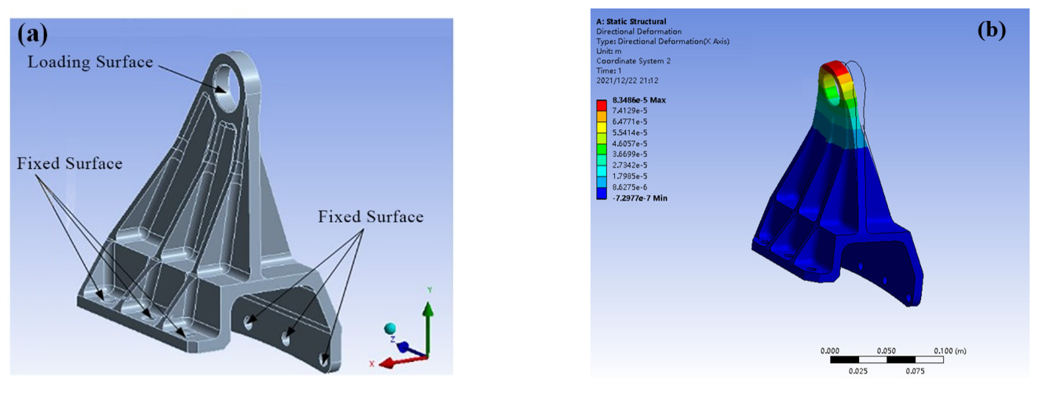
To obtain support stiffness of the mounting structure, the static analysis of each mounting structure is carried out via Workbench software. The support is modeled using solid187 elements and bolt holes connecting the support and casing that is set to be fixed (as shown in Figure 4a). Meanwhile, 1000 N force are applied at the mounting hole along the local coordinate axis x_A, y_A, and z_A, respectively, to obtain the axial displacement x_A = 0.083486 mm (as shown in Figure 4b), normal displacement y_A = 0.00128 mm, and tangential displacement z_A = 0.013327 mm of the top-left support A in the local coordinate system. Using the formula K = F/x, the axial stiffness k_Ax’ = F/x_A = 1000 N/0.083486 mm = 1.20 × 10⁷ (N/m), the normal stiffness k_Ay’ = F/y_A = 1000/0.00128 = 7.8 × 10⁸ (N/m), and the tangential stiffness k_Az’ = F/z_A = 1000 N/0.013327 mm = 7.5 × 10⁷ (N/m) of the top-left support A in the local coordinate system can be obtained. ${{\mathbf{K}}^{\mathbf{\prime }}}_{\mathbf{A}}$, ${{\mathbf{K}}^{\mathbf{\prime }}}_{\mathbf{B}}$, ${{\mathbf{K}}^{\mathbf{\prime }}}_{\mathbf{C}}$, and ${{\mathbf{K}}^{\mathsf{\prime }}}_{\mathbf{D}}$, respectively, represent the support stiffness under the local coordinate system of corresponding support. The support stiffness under the local coordinate system is shown in

Table 3. The stiffness of each support in the local coordinate system.

Stiffness (N/m)	Mount #
	A	B	C	D
kx’	1.20 × 107	1.00 × 107	5.40 × 106	1.30 × 107
ky’	7.80 × 108	2.60 × 108	3.50 × 108	3.60 × 108
kz’	7.50 × 107	3.70 × 108	1.50 × 108	2.50 × 108

.

The direction angles of x_A-axis in the global coordinate system are defined as ${\theta }_{x_{\mathrm{A}}x}$,${\theta }_{x_{\mathrm{A}}y}$, and ${\theta }_{x_{\mathrm{A}}z}$, which are the included angles between the x_A-axis and the x, y, and z axes, respectively. Further, their cosine values are defined as the direction cosine of x_A-axis. The direction cosines of the x_A axis can be described as:

$$n_{x_{\mathrm{A}}x}=\cos {\theta }_{x_{\mathrm{A}}x}$$

(11)

$$n_{x_{\mathrm{A}}y}=\cos {\theta }_{x_{\mathrm{A}}y}$$

(12)

$$n_{x_{\mathrm{A}}z}=\cos {\theta }_{x_{\mathrm{A}}z}$$

(13)

Correspondingly, the direction cosines of the y_A-axis is $n_{y_{\mathrm{A}}x}$, $n_{y_{\mathrm{A}}y}$, and $n_{y_{\mathrm{A}}z}$, and the direction cosines of the z_A-axis is $n_{z_{\mathrm{A}}x}$, $n_{z_{\mathrm{A}}y}$, and $n_{z_{\mathrm{A}}z}$. Combine all the direction cosines of the x, y, and z axes as the following matrix:

$$\mathbf{T}=\left(\begin{array}{ccc}{n}_{x_{\mathrm{A}}x}& n_{x_{\mathrm{A}}y}& n_{x_{\mathrm{A}}z}\\ n_{y_{\mathrm{A}}x}& n_{y_{\mathrm{A}}y}& n_{y_{\mathrm{A}}z}\\ n_{z_{\mathrm{A}}x}& n_{z_{\mathrm{A}}y}& n_{z_{\mathrm{A}}z}\end{array}\right)$$

(14)

where T is the coordinate transformation matrix.

The transformation relationship between the local coordinate system and the global coordinate system of the top-left support A can be written as:

$${\mathbf{T}}_A=\left(\begin{array}{ccc}\cos {\theta }_{x_{\mathrm{A}}x}& \cos {\theta }_{x_{\mathrm{A}}y}& \cos {\theta }_{x_{\mathrm{A}}z}\\ \cos {\theta }_{y_{\mathrm{A}}x}& \cos {\theta }_{y_{\mathrm{A}}y}& \cos {\theta }_{y_{\mathrm{A}}z}\\ \cos {\theta }_{z_{\mathrm{A}}x}& \cos {\theta }_{z_{\mathrm{A}}y}& \cos {\theta }_{z_{\mathrm{A}}z}\end{array}\right)=\left(\begin{array}{ccc}|\cos 4°|& |\cos 93°|& |\cos 88°|\\ |\cos 87°|& |\cos 8°|& |\cos 97°|\\ |\cos 92°|& |\cos 83°|& |\cos 8°|\end{array}\right)$$

(15)

The stiffness of the top-left support A in the global coordinate system can be obtained as:

$${\mathbf{K}}_{\mathbf{A}}={\mathbf{T}}_{\mathbf{A}}{{\mathbf{K}}^{\mathbf{\prime }}}_{\mathbf{A}}{\mathbf{T}}_{\mathbf{A}}^{\mathbf{T}}$$

(16)

Calculations of the stiffness of supports B, C, and D in the global coordinate system along the directions of the x, y, and z axes, as well as the stiffness of each support in the global coordinate system are listed in

Table 4. The stiffness of each support in the global coordinate system.

Stiffness (N/m)	Mount #
	A	B	C	D
kx	6.40 × 107	2.90 × 108	8.40 × 107	1.50 × 108
ky	9.10 × 108	2.80 × 109	4.00× 108	4.50 × 108
kz	2.00 × 108	3.90 × 109	1.70× 108	3.10 × 108

.

3.1.3. Natural Frequencies Calculation

According to the above-mentioned calculation, supports stiffness of the rigid body, supports location, and the first six natural frequencies of the rigid body system are calculated by the established dynamic model to be 576 Hz, 896 Hz, 1586 Hz, 1947 Hz, 2295 Hz, and 5655 Hz, respectively.

3.2. Modal Analysis and Model Verification

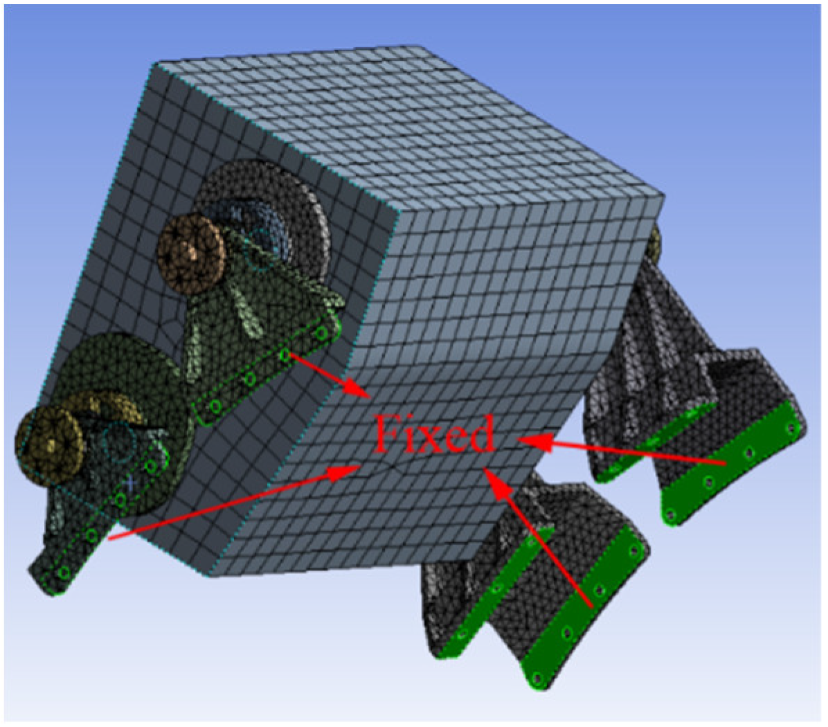
The simplified oil tank is modeled using solid187 elements, which are divided into 57,610 elements and 116,638 nodes. The oil tank body has a large stiffness and small deformation under working conditions. Therefore, its deformation is ignored in the numerical simulation and is considered as a rigid body [26]. The mounting pedestal components are flexible. There is friction contact between damping ring surface and connecting pin surface, as well as between the mounting pedestal lifting lug surface and connecting pin surface; the friction coefficient is 0.3. Fixed constraints are imposed on the bolt holes of each mounting pedestal. The finite element model (FEM) is established as Figure 5. The modal calculation results are obtained in

Table 5. The calculation results of the first six modes of the simplified rigid body model.

f1 = 565 HzTranslate along the x direction	f 2 = 916 Hz Translate along z direction of the left support
f3 = 1582 HzRotate along the y direction of top-right support	f4 = 1937 HzRotate along the x direction of right support
f5 = 2177 HzRotate along the y direction	f6 = 5376 HzLocal torsion of bottom-left support

via Block Lanczos modal extraction method.

The theoretical calculation and FE modal calculation results of the simplified rigid body model are shown in

Table 6. Results of theoretical calculation and FEM.

Order	Analytical Method (Hz)	FEM-ANSYS (Hz)	Error (%)
1	576	565	1.9%
2	896	916	2.2%
3	1586	1582	0.3%
4	1947	1937	0.5%
5	2295	2177	5.4%
6	5655	5376	5.2%

. The first six natural frequencies obtained by the two methods are consistent, indicating that the established dynamic model of a rigid body system with multi-point elastic supports is effective.

4. The Influence of Support Location on the System Inherent Characteristics

The variation of supports location will lead to the corresponding stiffness component of each support to change, which will further affect the system dynamic characteristics. The sensitivity of each support stiffness component to the variation of the corresponding support location is different. Ten different locations are selected within the adjustable range of each support, and the corresponding stiffness components are calculated to the first two natural system frequencies at different support locations. Next, the sensitivity of the system inherent characteristics is analyzed when the support location changes.

4.1. Determination of Each Support Spatial Location

Considering the size and assembly space constraints of the simplified rigid model with four supports, the value ranges of each support location (d_A = (d_Ax, d_Ay, and d_Az), d_B = (d_Bx, d_By, and d_Bz), d_C = (d_Cx, d_Cy, and d_Cz) and d_D = (d_Dx, d_Dy, and d_Dz)) are defined, as shown in

Table 7. Value ranges of each support location.

Location (mm)	Mount #
	A			B			C			D
	dAx	dAy	dAz	dBx	dBy	dBz	dCx	dCy	dCz	dDx	dDy	dDz
Max	−211	−125	−205	−211	−150	0	211	−125	−205	211	−150	0
Min	−211	180	0	−211	140	205	211	180	0	211	140	205

.

4.2. Calculation of the Corresponding Stiffness of Each Support at Different Spatial Locations

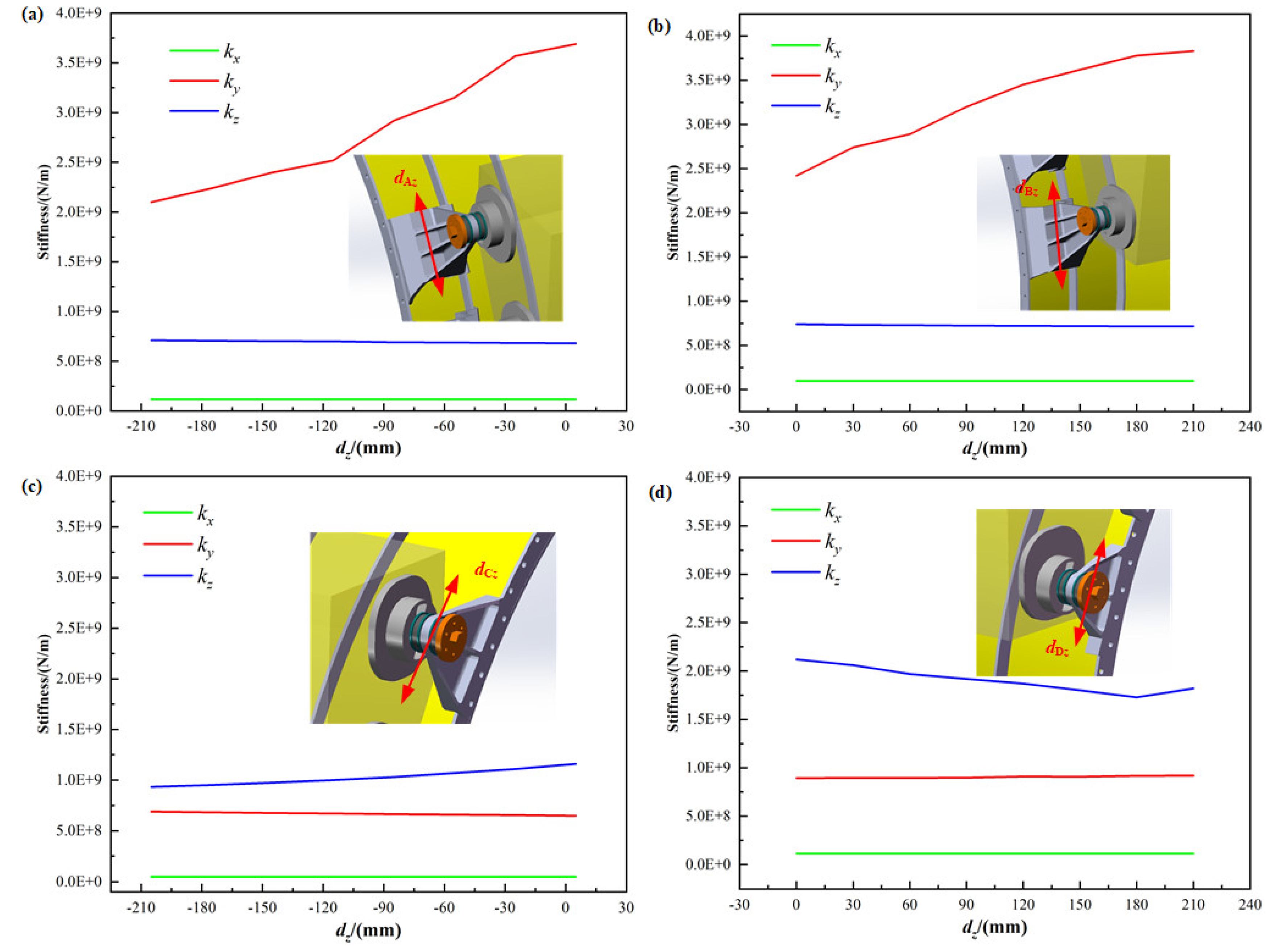
The influence of each support location variation on the stiffness components of each support is studied in this section. Considering the actual installation situation of the simplified rigid structure, the variation of each support stiffness component is analyzed when the corresponding tangential location d_z along the casing changes. Take ten mounting locations at equal intervals along the tangential position d_z of the casing and perform static analysis for each support at different locations. Calculate the local stiffness components of each support at corresponding locations, and then obtain the global stiffness components of each support at corresponding locations through coordinate conversion, as shown in Figure 6. Figure 6a–d show that the normal stiffness component k_y of the top-left support and the bottom-left support are more sensitive to the variation of the support locations.

4.3. Calculation of the System Natural Frequencies at Different Spatial Positions of Each Support

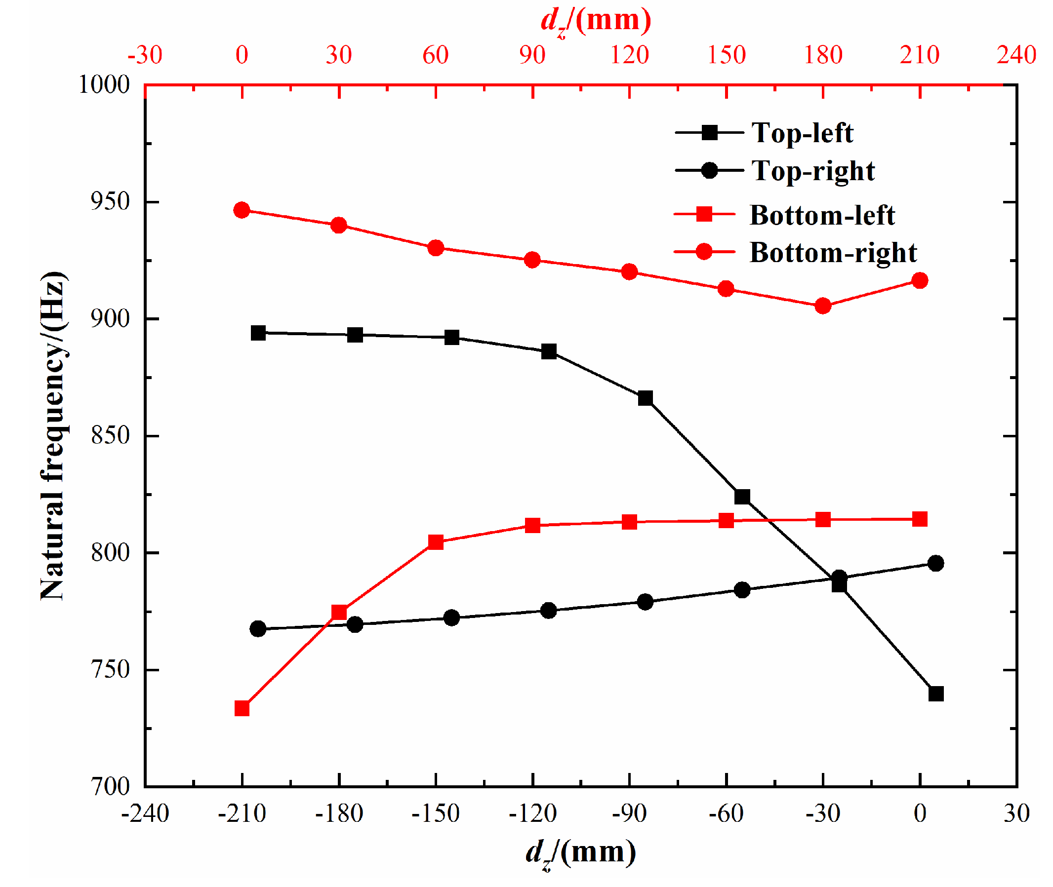
The influence of each support location variation on the system natural frequencies is studied in this section. Considering the actual installation situation of the simplified rigid structure, the variation of the system natural frequencies is analyzed when the corresponding tangential location d_z along the casing changes. The stiffness matrix K (Equation (10)) indicates that the variation of the normal stiffness component k_y mainly causes the change of the second systems order natural frequency, and only the variation curve of the second systems order natural frequency with different tangential location d_z of each support is given, as shown in Figure 7. It is observed that the second system order natural frequency is the most sensitive to the top-left support location, followed by the bottom-left support location. It can be known from the dynamic equation that the system natural frequencies are the results of the joint action of the support locations and the support stiffness. Comparing Figure 6a with Figure 7, variation trends of the stiffness and the second system frequency caused by top-left support locations is opposite. The increase of top-left support stiffness is to increase the system’s natural frequency; however, the system’s natural frequency decreases, which is due to the action of the top-left support location, further indicating that the system’s natural frequency is most sensitive to the variation of the top-left support location. The variation of the bottom-left support location leads to the increase of the system’s natural frequency, which is mainly due to the increase of the stiffness components caused by the change of the bottom-left support location.

5. RSM of Support Location Layout Optimization

5.1. Response Surface Methodology by Using Kriging Mode

RSM is adopted in dynamic analysis of the rigid body system with multi-point spatial supports, for the complex implicit relationship between objective functions and design variables. RSM is a collection of statistical and mathematical techniques useful for developing, improving, and optimizing processes in which a response of interest is influenced by several variables and where the objective is to optimize this response [27]. According to the Weierstrass Approximation Theorem, most functions can be approximated by polynomials. Therefore, the relationship between system response and design variables can approximately be expressed by the RSM, in order to avoid solving the complex equations directly.

The sampling method and fitting method are two crucial issues in RSM. Among many sampling methods, Monte Carlo sampling (MCS) has been widely used for the orthogonality and uniform spacing of sampling points [28]. The present Kriging model [29] was adopted to expresses the objective functions.

5.2. Modeling of Response Surface and Its Verification

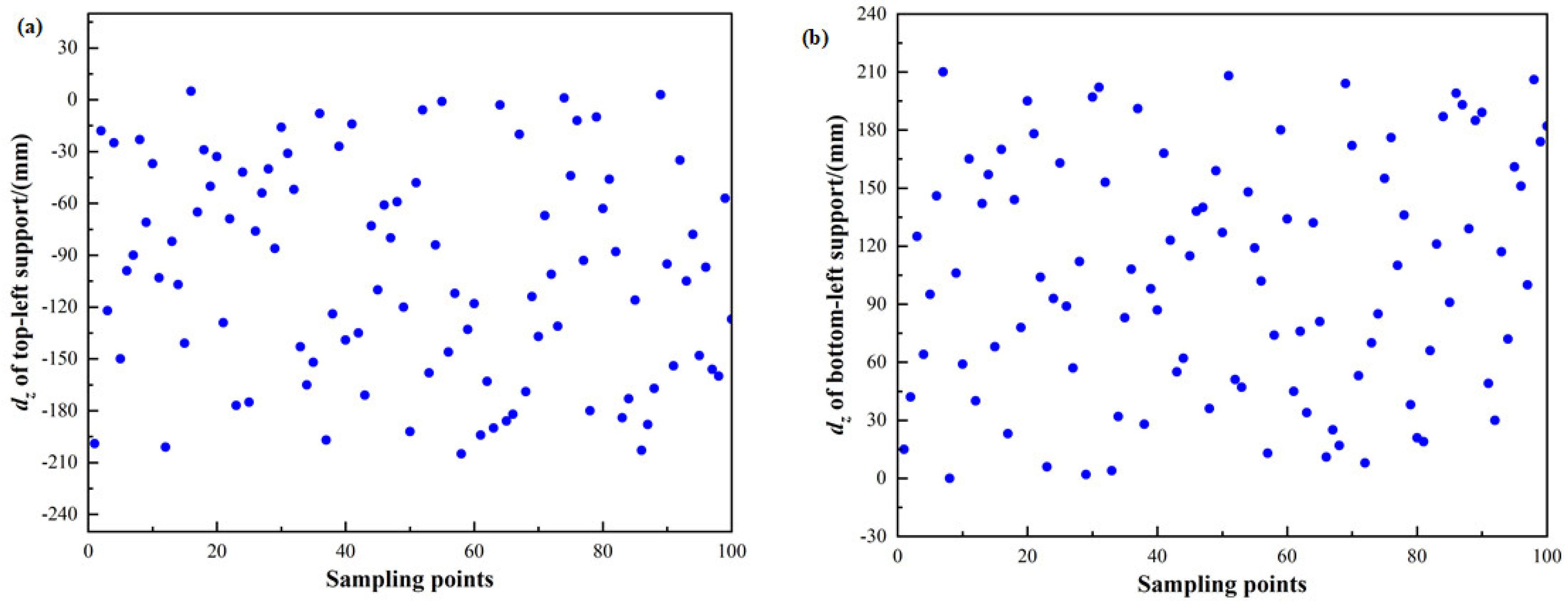
The Monte Carlo sampling method was used to obtain 100 sampling points in the constraint range of our design variables, as shown in Figure 8 and

Table 8. Values of sampling points and the corresponding objective functions.

Parameters	X1	X2	……	X99	X100
dAz/mm	−101	−71	……	−139	−31
dBz/mm	106	76	……	144	36
f1	395	395	……	395	394
f2	557	556	……	558	555
f3	868	806	……	940	745
f4	952	950	……	955	949
f5	1148	1140	……	1181	1152
f6	2006	2007	……	2003	2011

. The corresponding support stiffness components were calculated according to the support locations sampling points and by substituting values of the corresponding support stiffness components into the analytical dynamic model of the rigid body system with spatial multi-point supports; values of the system first six natural frequencies were obtained, which are also listed in Table 8.

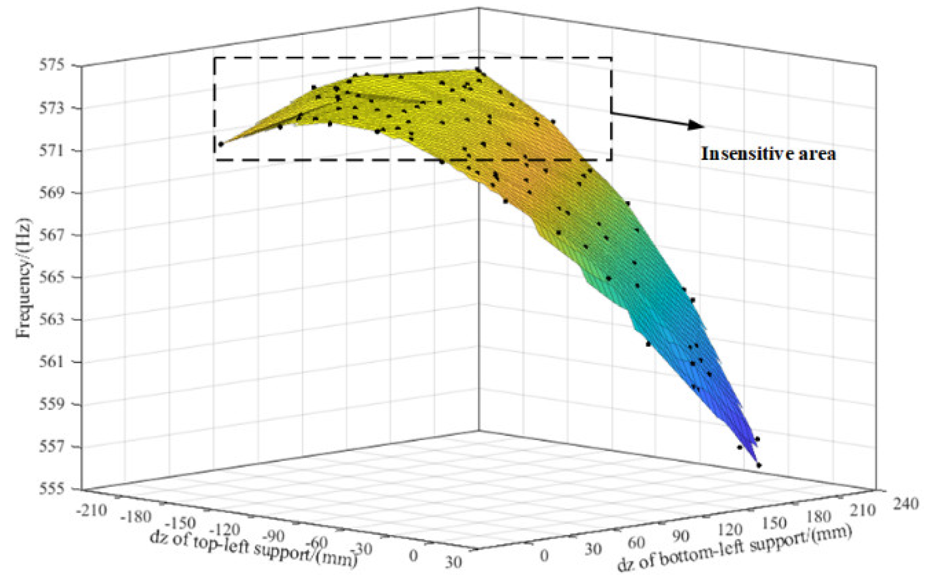
Next, the RSM (illustrated in Figure 9) can be obtained by using the Kriging model coupled with the Gauss correlation function. To validate the obtained RSM, three groups of validation sampling points are reselected by MCS and substituted into analytic method (AM) and RSM, respectively. The results are obtained as listed in

Table 9. Values of objective functions obtained by AM and RSM.

	X1			X2			X3
dAz/mm	−177			−76			−23
dBz/mm	165			59			114
f1	AM	RSM	Error	AM	RSM	Error	AM	RSM	Error
	573	573	0	573	572	0.17%	566	566	0
f2	AM	RSM	Error	AM	RSM	Error	AM	RSM	Error
	905	905	0	879	879	0	883	883	0
f3	AM	RSM	Error	AM	RSM	Error	AM	RSM	Error
	1757	1757	0	1234	1232	0.16%	1278	1274	0.31%
f4	AM	RSM	Error	AM	RSM	Error	AM	RSM	Error
	1875	1876	0.05%	1786	1787	0.06%	1821	1820	0.05%
f5	AM	RSM	Error	AM	RSM	Error	AM	RSM	Error
	2579	2580	0.04%	1843	1844	0.05%	1848	1855	0.38%
f6	AM	RSM	Error	AM	RSM	Error	AM	RSM	Error
	4047	4050	0.07%	3985	3971	0.35%	4384	4376	0.18%

. It reveals that the differences of results by these two methods are within 1%, which indicates the sufficient accuracy of RSM.

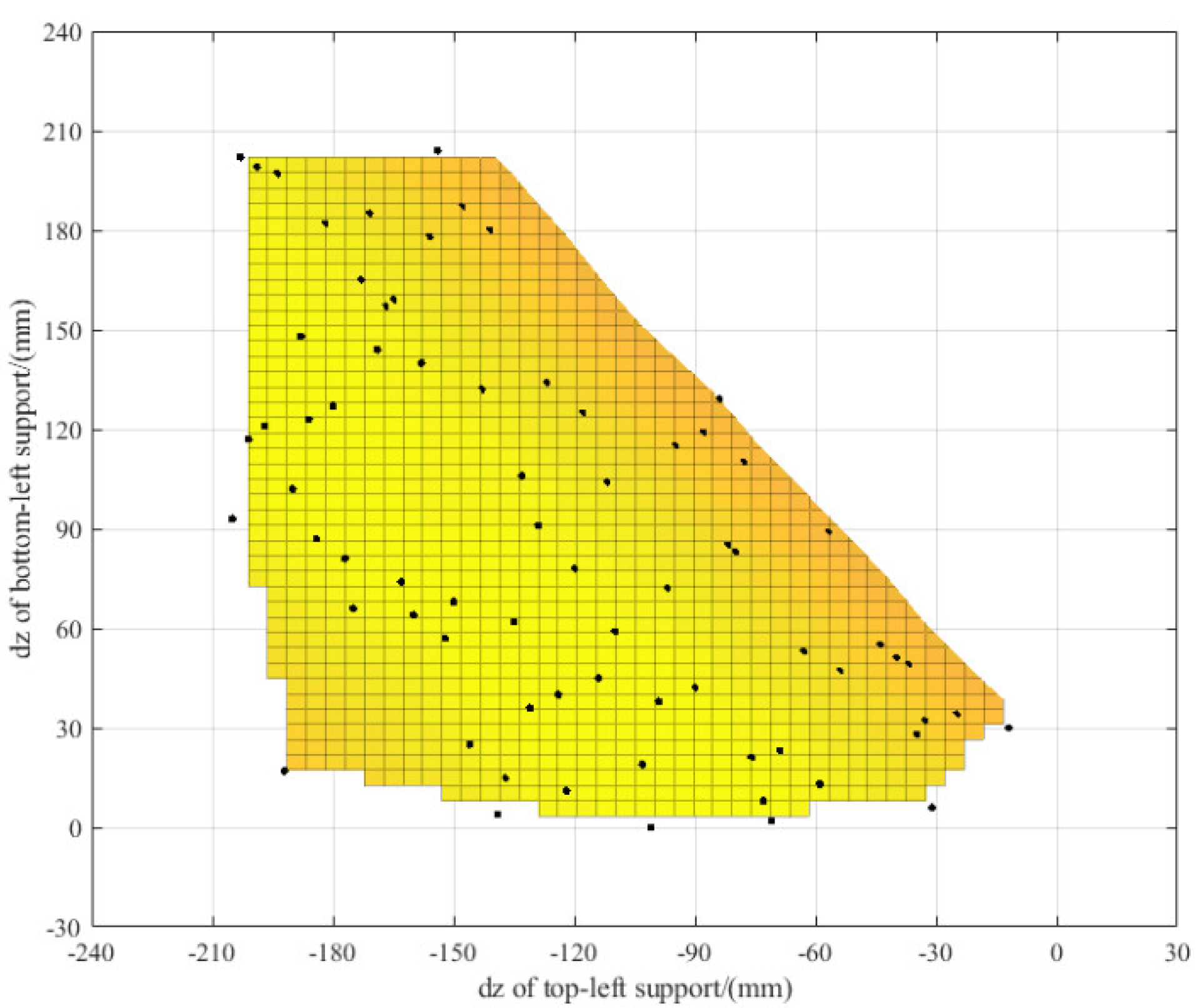
5.3. Support Spatial Location of the System Mode Insensitive Region

According to the obtained RSM, the mode insensitive region (as shown Figure 9) of a simplified rigid body system with four supports was obtained. The allowable variation area of the given support spatial location was shown in Figure 10.

6. The Influence of Support Stiffness on the System Inherent Characteristics

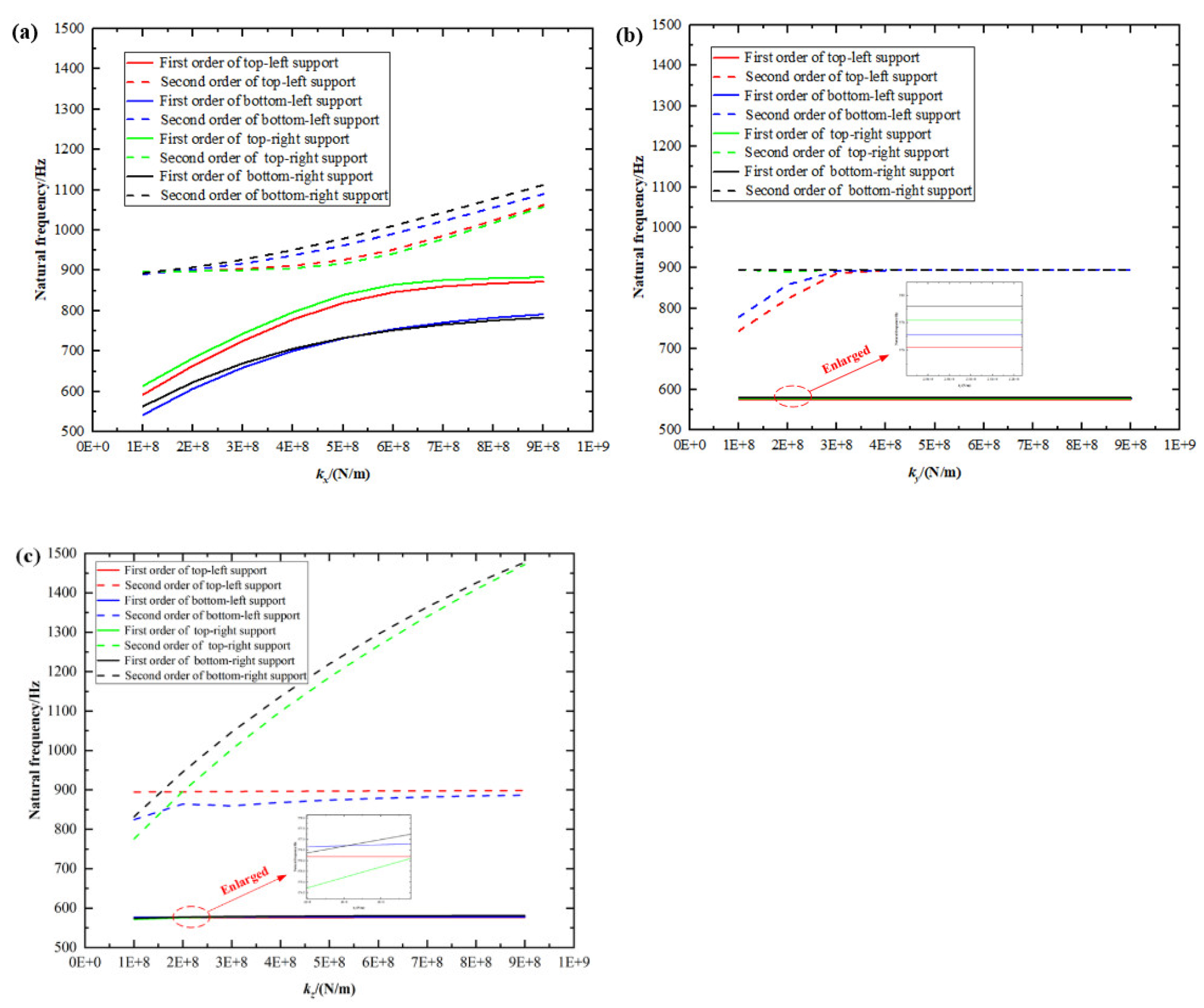
Taking a simplified rigid body system with four supports as an example, the influence of each support stiffness on the system’s inherent characteristics was studied. The stiffness range of each support was from 1 × 10⁸ (N/m) to 9 × 10⁸ (N/m), and the first two natural frequencies of a simplified rigid body system under the corresponding stiffness were calculated. Figure 11a–c shows the variation curves of the first two natural frequencies of a simplified rigid body system when the axial stiffness k_x, normal stiffness k_y and tangential stiffness k_z of each support change, where the solid line represents the first order frequency, and the dotted line represents the second order frequency. It can be observed that the system dynamic characteristics are most sensitive to the axial stiffness k_x of the four supports, followed by the tangential stiffness k_z, and least sensitive to the normal stiffness k_y. This is due to the axial distance (d_nx) from each support to the center of mass being larger than the normal distance (d_ny) and the tangential distance (d_nz), resulting in a more obvious moment of inertia effect, which further affects the system’s inherent characteristics. From Figure 11a, the sensitivity of system dynamic characteristics is similar to the axial stiffness, k_x, of the four supports.

7. Conclusions

In this paper, the modal characteristics of the rigid body system with multi-point spatial supports are conducted. The kinetic equation of the rigid body system with multi-point spatial supports is derived through the energy method. A good agreement is obtained by validating both the analytic method and the FEM results. The effects of spatial location and stiffness components of each support are all illustrated. Some conclusions and new results are obtained as follows:

• The spatial location components of each support have a remarkable effect on the modal frequencies. Since the variation of the spatial location of each support will cause the variation of the stiffness component of the support, and further the inherent characteristics of the system are affected. The case study shows that the second order natural frequency of the lubricant tank system is most sensitive to the location variation of the top-left support, followed by the bottom-left support. Next, the first order natural frequency RSM of the lubricant tank system is established, and the allowable variation range of the support spatial location corresponding to the mode insensitive region (allowable variation of plus or minus 1%) of the lubricant tank system with four supports is obtained.
• The dynamic characteristics of the lubricant tank system are very sensitive to the axial stiffness (k_x) of each support, followed by the tangential stiffness (k_z), and the least sensitive to the normal stiffness (k_y).
• From an engineering point of view, the above results could be used to guide the dynamic design of the rigid structural system to avoid resonance. In the dynamic design of the lubricant tank system mentioned in present work, either axial stiffness (k_x) of each support or the location variation of the top-left support and the bottom-left support can be designed to avoid resonance. The suggested adjustable range of each support axial stiffness (k_x) can be 1 × 10⁸ N/m–9 × 10⁸ N/m, and the suggested adjustable range of location variation of the top-left support (d_Az) and the bottom-left support (d_Bz)can be (−5,0) and (200,205), respectively.

References

- Shangguan, W.B. Engine mounts and powertrain mounting systems: A review. Int. J. Veh. Des. 2009, 49, 237–258. [Google Scholar] [CrossRef]
- Mrad, F.L.; Machado, D.M.; Horta, G.J.; Sad, A.U. Optimization of the vibrational comfort of passenger vehicles through improvement of suspension and engine rubber mounting setups. Shock Vib. 2018, 17, 9861052. [Google Scholar] [CrossRef]
- Li, J.; Gao, Z.; Huang, J.; Zhao, K. Aerodynamic design optimization of nacelle/pylon position on an aircraft. Chin. J. Aeronaut. 2013, 26, 850–857. [Google Scholar] [CrossRef] [Green Version]
- Angrosch, B.; Plöchl, M.; Reinalter, W. Mode decoupling concepts of an engine mount system for practical application. Proc. Inst. Mech. Eng. Part K J. Multi-Body Dyn. 2015, 229, 331–343. [Google Scholar] [CrossRef]
- Liang, J.; Zhang, D.; Wang, S. Vibration characteristic analysis of single-cylinder two-stroke engine and mounting system optimization design. Sci. Prog. 2020, 103, 003685042093063. [Google Scholar] [CrossRef]
- Mirza, N.; Hussain, K.; Day, A.J.; Klaps, J. Effect of component stiffness and deformation on vehicle lateral drift during braking. Proc. Inst. Mech. Eng. Part K J. Multi-Body Dyn. 2009, 223, 9–22. [Google Scholar] [CrossRef]
- Jeong, T.; Singh, R. Analytical methods of decoupling the automotive engine torque roll axis. J. Sound Vib. 2000, 234, 85–114. [Google Scholar] [CrossRef] [Green Version]
- Park, J.-Y.; Singh, R. Effect of non-proportional damping on the torque roll axis decoupling of an engine mounting system. J. Sound Vib. 2008, 313, 841–857. [Google Scholar] [CrossRef]
- Tao, J.; Liu, G.; Lam, K. Design optimization of marine engine-mount system. J. Sound Vib. 2000, 235, 477–494. [Google Scholar] [CrossRef]
- Yu, Y.; Naganathan, N.G.; Dukkipati, R.V. A literature review of automotive vehicle engine mounting systems. Mech. Mach. Theory 2001, 36, 123–142. [Google Scholar] [CrossRef]
- Zhang, B.; Zhan, H.; Gu, Y. A general approach to tune the vibration properties of the mounting system in the high-speed and heavy-duty engine. J. Vib. Control. 2014, 22, 247–257. [Google Scholar] [CrossRef] [Green Version]
- Lee, D.; Brennan, M.J.; Mace, B.R. Vibration isolation of a marine diesel generator set. Noise Control. Eng. J. 2007, 55, 183. [Google Scholar] [CrossRef]
- Snowdon, J.C. Vibration isolation: Use and characterization. J. Acoust. Soc. Am. 1979, 68, 1245–1274. [Google Scholar] [CrossRef]
- Xiong, Y.; Kongjie, S. Power flow analysis for a new isolation system flexible floating raft. Chin. J. Mech. Eng. 1996, 9, 260–264. [Google Scholar]
- Li, Q.C.; Zhou, R. Research of vibration characteristics of ship propeller-shaft longitudinal two-stage vibration isolation system. J. Phys. Conf. Ser. 2021, 1939, 012103. [Google Scholar] [CrossRef]
- Hu, F.C.; Yang, J.G.; Zhong, Q.M. Analysis and experiment research on two layers vibration isolation of diesel generating set in “superiority” oil tanker. In Proceedings of the 8th International Conference on Electronic Measurement and Instruments, Xi’an, China, 16–18 August 2007; pp. 704–710. [Google Scholar]
- Lv, Z.Q.; He, L.; Shuai, C.G. Optimization of natural frequencies of large-scale two-stage raft system. In Proceedings of the 13th International Conference on Motion and Vibration Control/12th International Conference on Recent Advances in Structural Dynamics, Southampton, UK, 4–6 July 2016; IOP: Southampton, UK, 2016; pp. 1–8. [Google Scholar]
- Junchuan, N.; Kongjie, S.; Rui, H. Study on strategies of active vibration isolation in the coupling flexible system. Chin. J. Mech. Eng. 2001, 37, 28–33. [Google Scholar]
- Wang, Q.; Zeng, J.; Wu, Y.; Zhu, B. Study on semi-active suspension applied on carbody underneath suspended system of high-speed railway vehicle. J. Vib. Control. 2020, 26, 671–679. [Google Scholar] [CrossRef]
- Niu, J.; Song, K.; Lim, C. On active vibration isolation of floating raft system. J. Sound Vib. 2005, 285, 391–406. [Google Scholar] [CrossRef]
- Foumani, M.; Khajepour, A.; Durali, M. Application of Sensitivity Analysis to the Development of High Performance Adaptive Hydraulic Engine Mounts. Veh. Syst. Dyn. 2003, 39, 257–278. [Google Scholar] [CrossRef]
- Saitoh, T.; Kim, H.; Takenaka, K.; Nakahashi, K. Multi-point aerodynamic design optimization of DLR F-6 Wing-body-nacelle-pylon configuration. Int. J. Aeronaut. Space Sci. 2017, 18, 403–413. [Google Scholar] [CrossRef]
- Epstein, B.; Peigin, S. Automatic Optimization of Wing–Body–Under-the-Wing-Mounted-Nacelle Configurations. J. Aircr. 2016, 53, 691–700. [Google Scholar] [CrossRef]
- Li, W.F. Dynamics and Vibration Fatigue Analysis of Liquid Sloshing in an Aircraft Fuel Tank. Ph.D. Thesis, Nanjing University of Aeronautics and Astronautics, Nanjing, China, 2014. [Google Scholar]
- Baeten, A.; Stern, D. Prediction of highly dynamic airborne tank fuel sloshing and impact effects. In Proceedings of the 46th AIAA Aerospace Sciences Meeting and Exhibit, Reno, Nevada, 7–10 January 2008; pp. 1–15. [Google Scholar]
- Wang, Y.; Zhou, C.H.; Zhou, Y.; Xu, S.L.; Wang, B.; Li, Y.W.; Liu, Z.H. Design of bracket of oil tank assembly in aero-engine based on topology optimization. J. Propuls. Technol 2021, 1–12. [Google Scholar] [CrossRef]
- Johnson, C.D.; Kienholz, D.A. Finite element prediction of damping in structures with constrained viscoelastic layers. AIAA J. 2012, 20, 1284–1290. [Google Scholar] [CrossRef]
- Janssen, H. Monte-Carlo based uncertainty analysis: Sampling efficiency and sampling convergence. Reliab. Eng. Syst. Saf. 2013, 109, 123–132. [Google Scholar] [CrossRef]
- Han, Z. Kriging surrogate model and its application to design optimization: A review of recent progress. Acta Aeronaut. Astronaut. Sin. 2016, 37, 3197–3225. [Google Scholar]
Figure 1.
Definition of a rigid body system with multi-point elastic supports and its motion: (a) the definition of the global coordinate system of a rigid body and the local coordinate system of each support; (b) motion definition of the rigid body.
Figure 2.
The definition of each support spatial location and its stiffness decomposition (take the top-left support A as an example): (a) definition of each support spatial location; (b) support stiffness decomposition.