
Control Chart Concurrent Pattern Classification Using Multi-Label Convolutional Neural Networks


1
Department of Industrial Engineering and Management, Yuan Ze University, No. 135, Yuan-Tung Road, Chung-Li District, Taoyuan City 32003, Taiwan
2
Scandinavian Health Limited, No. 36, Liufu Road, Luzhu District, Taoyuan City 338, Taiwan
3
Unimicron Technology Corp., No. 179, Shanying Road, Guishan Ind. Park, Taoyuan City 33341, Taiwan
*
Author to whom correspondence should be addressed.
Appl. Sci. 2022, 12(2), 787; https://0-doi-org.brum.beds.ac.uk/10.3390/app12020787
Submission received: 16 December 2021
/
Revised: 7 January 2022
/
Accepted: 10 January 2022
/
Published: 13 January 2022
(This article belongs to the Special Issue Smart Service Technology for Industrial Applications)
Abstract
:The detection and identification of non-random patterns is an important task in statistical process control (SPC). When a non-random pattern appears on a control chart, it means that there are assignable causes which will gradually deteriorate the process quality. In addition to the study of a single pattern, many researchers have also studied concurrent non-random patterns. Although concurrent patterns have multiple characteristics from different basic patterns, most studies have treated them as a special pattern and used the multi-class classifier to perform the classification work. This study proposed a new method that uses a multi-label convolutional neural network to construct a classifier for concurrent patterns of a control chart. This study used data from previous studies to evaluate the effectiveness of the proposed method with appropriate multi-label classification metrics. The results of the study show that the recognition performance of multi-label convolutional neural network is better than traditional machine learning algorithms. This study also used real-world data to demonstrate the applicability of the proposed method to online monitoring. This study aids in the further realization of smart SPC.
1. Introduction
Control charts are a statistical process control (SPC) tool used to determine if a manufacturing or business process is behaving as intended. When a non-random pattern appears on the control chart, it suggests that there exist one or more assignable causes which will gradually deteriorate the process/product quality. The presence of assignable causes requires instant investigation of the process, including the identification of root causes and implementing corrective actions. It was recognized that non-random patterns can provide relevant information about process diagnosis. Montgomery [1] pointed out that every non-random pattern is mapped to a set of assignable causes. Therefore, if the pattern type can be correctly recognized and identified, it will help to diagnose the possible causes of the manufacturing process problem.
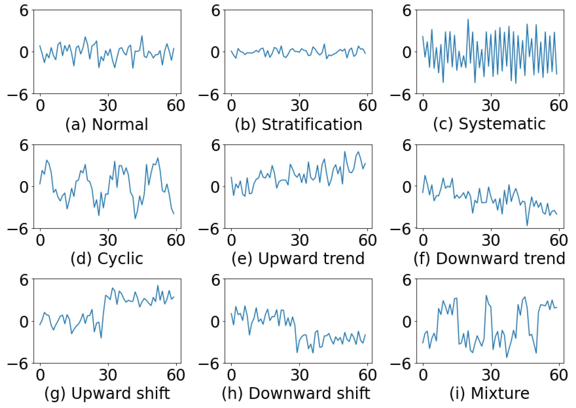
The statistical quality control manual of the Western Electric Company [2] first described the non-random patterns that often appeared on control charts, and proposed a set of zone tests for analyzing the patterns. Figure 1 illustrates several representative examples of control chart patterns. A normal pattern (NOR) only exhibits random variations (Figure 1a). In stratification (STRA), the points tend to cluster around the center line. Figure 1b illustrates an example of stratification. In systematic variations (SYS), a high point is always followed by a low one or vice versa (Figure 1c). A cycle (CYC) can be recognized by a series of high portions or peaks interspersed with low portions or troughs. A typical example is shown in Figure 1d. A trend is characterized by a continuous movement in one direction. Figure 1e illustrates an upward trend (UT) and Figure 1f a downward trend (DT). A shift is a sudden or abrupt change in the average of the process. Figure 1g depicts an upward shift (US) and Figure 1h a downward shift (DS). In a mixture (MIX) pattern, the points tend to fall near the high and low edge of the pattern with an absence of points near the center (Figure 1i). A mixture is caused by the combination of data from two or more distributions.
Nelson [3,4] also proposed a set of runs rules for analyzing non-random patterns of control charts. Zone tests and runs rules are usually referred to as sensitizing rules or supplementary rules [1]. These rules are easy to use and have been adopted in many statistical packages (e.g., Minitab). However, the application of the aforementioned sensitizing rules is not without its drawbacks, because no one-to-one mapping between the rules and non-random patterns exists [5].
In response to the limitations of the sensitizing rules, many researchers have applied pattern recognition to the analysis of control chart patterns [5,6,7,8]. In the past, researchers have used machine learning (ML) algorithms to build pattern classifiers to identify non-random patterns in manufacturing process data. The task is commonly referred to as control chart pattern recognition (CCPR). Zorriassatine and Tannock [9] comprehensively reviewed the literature on the application of neural networks to SPC. Perry and Pignatiello [10] and Barghash [11] reviewed the literature on the application of neural networks in CCPR. Hachicha and Ghorbel [12] discussed recent research on control chart patterns and proposed some directions for future research. With the development of the industrial internet of things (IIOTs) and artificial intelligence (AI), collecting process data and applying intelligent decision-making models for analysis have become more feasible than before. Researchers have focused on using advanced methods to improve the accuracy of CCPR. In the following, we provide a summary and analysis of the relevant publications on the topic of control chart pattern recognition.
In research on CCPR, the pattern can be expressed in the form of original data or features [12]. Most methods that use features have relied on hand-crafted features, including shape features [13,14,15], multi-resolution wavelet features [16] and statistical features [17]. Classification methods include rule-based methods [6], decision trees [18,19], neural networks [5,20,21], and support vector machines [22,23]. Recently, deep learning (DL) techniques have demonstrated strong capabilities in time series classification, and many studies have begun to focus on the application of deep learning techniques to the classification of control chart patterns [24,25,26,27,28].
Studies have focused on the identification of basic non-random patterns and, increasingly, on the identification of concurrent patterns (which are combinations of two or more basic patterns appearing simultaneously) [21,23,29,30,31]. A concurrent pattern indicates that the manufacturing process is affected by multiple assignable causes. To identify concurrent non-random patterns, researchers have often performed pre-processing to smooth the data or extract features. Some examples of pre-processing methods include a wavelet analysis [29,32,33], independent component analysis [34], and singular spectrum analysis [35,36].
This study proposed a novel method of classifying single and concurrent non-random patterns on control charts through the use of a convolutional neural network (CNN) to build a multi-label classifier. To the best of our knowledge, this study is the first to apply a multi-label CNN classifier to control chart concurrent pattern classification. The main ideas of using multi-label CNN are explained as follows.
CNNs are most commonly applied to computer vision [37,38,39]. Recently, researchers have demonstrated that it is possible to apply CNNs not only to image recognition tasks but also to time series classification tasks [40,41], which is called one-dimensional convolutional neural network (1D CNN). The primary advantage of CNNs is their ability to automatically learn the important features of a dataset without any hand-crafted feature extraction. The end-to-end classification system performs feature extraction jointly with classification. More importantly, CNN has the ability to learn the translation invariance features from the input [42,43]. For CCPR, the translation invariance means that the classifier can recognize the pattern regardless of where it appears in the window. This characteristic is extremely important when considering the dynamic nature of the non-random patterns [12].
In previous work, researchers have generally applied multi-class classifiers to concurrent CCPR. This is because a concurrent pattern is treated as a single pattern class. Because a concurrent pattern possesses multiple features, the classification algorithm must allow each sample to have more than one class label. The introduction of multi-label classification into concurrent CCPR is advantageous because the multi-label classification algorithm can predict more than one class label and has a chance of being partially correct; at least one nonrandom pattern being reported is preferable to no pattern being reported.
In this study, a multi-label 1D CNN was developed to analyze control chart patterns, and a series of experiments were conducted to assess the performance of the multi-label 1D CNN. The CNN was evaluated using real-world data and datasets from previous studies against traditional classifiers. The method presented here may contribute to the implementation of smart SPC.
The organization of the paper is as follows. Section 2 presents the proposed end-to-end multi-label 1D CNN architecture and a brief description of the traditional classifiers evaluated in this study. Subsequently, a set of performance metrics suitable for multi-label classification is given. Section 3 details the evaluation of the proposed approach against traditional classifiers. Section 4 presents the application of the proposed approach to real-world data from industry. Finally, the study is concluded and directions for future research are discussed.
2. Methods
This section describes the multi-label convolutional neural network used in this study and various performance metrics for evaluating multi-label classification. For the purpose of comparison, a brief review of traditional classifiers is also provided.
2.1. Convolutional Neural Network (CNN)
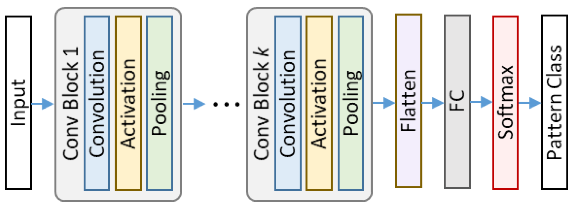
A typical CNN comprises of a convolution layer, a pooling layer, and one or more fully connected (FC) layers. The convolution layer is the key element in the CNN architecture. Its function is to perform feature extraction, including linear and non-linear operations (i.e., convolution operations and activation functions). The combination of convolution layer, activation layer, and pooling layer is usually referred to as the convolution block. In brief, the CNN network extracts features using the convolution blocks and performs classification using the fully connected layers. They join to form an end-to-end classifier that can reduce traditional feature engineering demands. Figure 2 illustrates a typical CNN architecture.
In the convolution block, the 1D convolution layer is used to extract feature maps and different numbers of 1D convolution filters of the same size are applied in each layer. Deeper convolution blocks have more convolution filters. The distance between two consecutive filter positions is called a stride and is usually set to 1. During the convolution operation, zero padding is typically used to avoid the loss of spatial dimensions. When a convolution layer is applied, the hyperparameters that must be determined include filter size and filter number.
The output of the convolution operation is passed to a non-linear activation function. Some commonly used functions include the identity, sigmoid, hyperbolic tangent (tanH), and rectified linear unit (ReLU) functions. The pooling layer is equivalent to a non-linear form of down sampling. Pooling comes in many forms, of which max pooling with a size of and a stride of 2 is most commonly used. The pooling layer can reduce the dimensionality of the feature map, and thus can exhibit translation invariance for small offsets and deformations.
The output feature map of the last convolutional layer or pooling layer is flattened, that is, it is converted into a 1D vector and connected to one or more fully connected layers. The number of neurons in a fully connected layer is typically determined through experimentation. In a classification problem, the number of neurons in the last layer of the network is equal to the number of classes. Softmax is usually chosen as the activation function of the last layer of the model. The Softmax function normalizes output values from the last fully connected layer to target class probabilities, where each value ranges between 0 and 1 and all values sum to 1. Each value in the output of the Softmax function can be interpreted as the probability of membership for each class. The class label of the maximum probability is selected as the output. The predicted output can be written as follows:
where is the activation value of the last layer neurons, the activation value of neuron is , is the number of classes and the number of last layer neurons, and is the label of the predicted class.
During training, the network finds the weights of the filter and the weights in the fully connected layer to minimize the difference between the true class label of the sample in the training set and the predicted value of the network. The most critical elements of training are the loss function and the optimization algorithm. Classification loss is calculated by comparing the class probabilities () and true labels of samples (). For multi-class classification, the loss calculated by the commonly used categorical cross-entropy loss function can be expressed as follows:
Gradient descent is often used as an optimization algorithm to iteratively update the learnable parameters (referring to the weights of the filter and the weights of the fully connected layer) in the network to minimize the loss. Some commonly used optimization algorithms include Stochastic Gradient Descent (SGD), RMSprop (Root Mean Square Prop) and Adam (Adaptive Moment Estimation) [44].
Overfitting is an important problem in machine learning. Several methods have been proposed to minimize overfitting [45]. Increasing the number of samples is one means of reducing overfitting. Other solutions include regularization with dropout or weight decay, batch normalization, and data augmentation, as well as the reduction in architectural complexity.
Data augmentation involves the random transformation of the original training data. Batch normalization normalizes the input of each layer according to the statistics obtained from the batch of data. This approach enables the use of a larger learning rate, while also reducing dependence on the initial value of the network weight. Dropout is a regularization method. During training, the randomly selected activations are set to zero, which can make the model less sensitive to specific weights in the network. Weight decay is also called regularization. The norm of the weights is added to the loss function. This penalizes the larger weights in a model and prompts the model to use smaller weights to reduce overfitting. Reducing the complexity of the model is also a feasible means to lessen overfitting. This can be performed by removing the layers or reducing the number of neurons.
2.2. Multi-Label Convolutional Neural Network
Multi-label classification is a classification problem in which multiple target labels can be assigned to each sample (instance). In multi-class classification, each sample can only be assigned to a single class. Researchers have proposed various methods to deal with multi-label classification problems, including the problem transformation method and algorithm adaptation [46]. The present study considers the latter method.
The multi-label classification problem is equivalent to building a model to map the input vector to a binary value vector . Each element of the vector is assigned a value of 0 or 1, which represents whether the label appears. In multi-label classification, a data sample can belong to multiple classes. With slight modification, a multi-class CNN can be applied to a multi-label classification problem.
One element that must be modified is the activation function of the last layer of the network. In multi-class classification, the Softmax function is generally used. However, the Softmax function considers the scores of the last layer of neurons, and then converts the scores into probabilities that sum to one. In multi-label classification, to make the output of each class independent, the sigmoid function must be used as the activation function for the last layer of neurons. The sigmoid function converts the score of the last layer of neurons to a value between 0 and 1 independently, without being affected by the scores of other neurons. If the output of a certain class is greater than the preset threshold (usually 0.5), the sample data are classified into that class. Because several classes may have outputs greater than the threshold, the sample data can be classified into more than one class.
Another element that must be changed is the type of loss function. In multi-class classification, the categorical cross-entropy is typically chosen as the loss function. In the multi-label classification, the use of binary cross-entropy allows the network to independently optimize the loss of each class.
2.3. Traditional Machine Learning Algorithms
2.3.1. Support Vector Machines
Support vector machines (SVMs) are a set of supervised learning methods that can be used for solving both classification and regression problems [47]. The algorithm used for classification is usually referred to as SVC and that used for regression is called SVR. In this section, we introduce the principles of SVC, which is relevant to this research. SVC is based on the margin maximization principle. It performs structural risk minimization, which improves the complexity of the classifier with the aim of achieving excellent generalization performance. The basic objective of this technique is to project nonlinear separable samples onto another higher dimensional space by using different types of kernel functions. The SVC algorithm accomplishes the classification task by constructing an optimal hyperplane that separates the data into categories in a higher dimensional space. SVC was first designed for binary classification. Nevertheless, it can be adapted for multi-class classification using the one-vs-one or one-vs-rest (OVR) method [48]. OVR is a heuristic approach for using binary classification algorithms in performing multi-class classification. It involves splitting the multi-class dataset into multiple binary classification problems. The one-vs-one strategy splits a multi-class classification into one binary classification problem per each pair of classes. To optimize classification performance, the SVC classifier parameters, kernel width , and regularization constant must be properly chosen.
2.3.2. Random Forest
Random forest (RF) is a machine learning technique that can be used to solve regression and classification problems [49]. It utilizes ensemble learning, which is a technique that combines many classifiers to provide solutions to complex problems. RF involves constructing numerous decision trees using bootstrap samples from the training dataset. RF also involves selecting a subset of input features at each split point in the construction of trees. For regression problems, prediction is the average prediction across the decision trees. A prediction on a classification problem is the majority vote for the class label across the trees in the ensemble.
The most important hyperparameter to tune for the RF is the number of random features to consider at each split point. In the regression context, Breiman [49] suggests setting the number of random features to be one-third of the number of predictors. For classification problems, Breiman [49] recommends setting this hyperparameter to be the square root of the number of features. The number of trees is another key hyperparameter to configure for the RF. Typically, the number of trees is increased until the model performance stabilizes. A final key hyperparameter is the maximum depth of decision trees used in the ensemble. Although the use of deeper trees increases accuracy, it also increases the likelihood of overfitting.
2.4. Performance Metrics
The performance metrics for multi-label classification models are different from those for multi-class classification problems. A recent survey of multi-label metrics and unified view of them is given by Wu and Zhou [50]. In this subsection, the metrics used in this study are reviewed. Let be the true set of labels for instance , be the predicted set of labels. Suppose is the number of instances. The symbol represents the 0 norm ( norm), which refers to the number of non-zero elements in the vector. All of the following evaluation metrics are defined on a per instance basis and the aggregate value is an average over all instances.
- Hamming loss
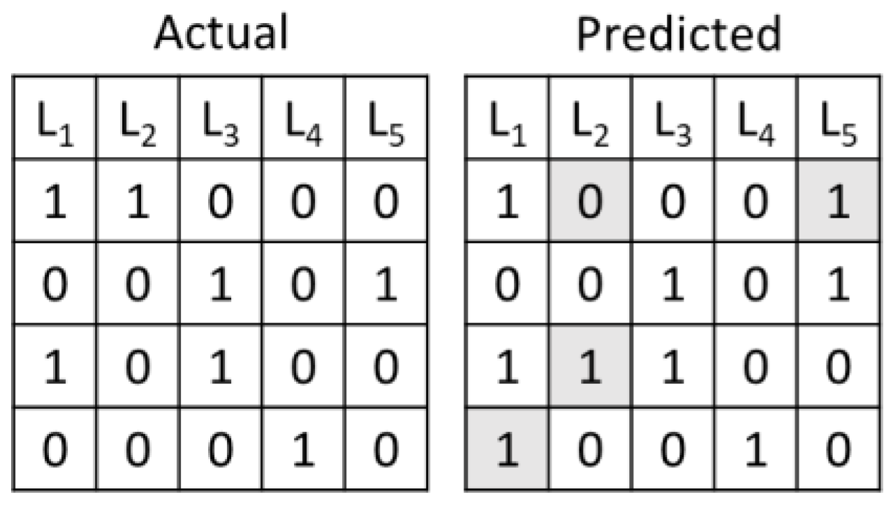
Hamming loss is the fraction of the incorrect labels to the total number of labels, i.e.,
where and are the element of the true label set and predicted label set for the instance, respectively. is the indicator function. The quantity is the total number of classes. The smaller the value of Hamming loss, the better the performance of the learning algorithm. The optimal value of Hamming loss function is 0. Figure 3 illustrates an example of Hamming loss. The loss in this example is calculated as 4/20. It can be interpreted as the fraction of wrong labels to the total number of labels.
- b.
- Jaccard index
The Jaccard index is defined as the number of correctly predicted labels divided by the union of the true and the predicted labels. It ranges from 0 to 1, and 1 is the perfect score.
- c.
- Precision and recall
Precision is defined as follows:
Recall is defined as follows:
- d.
- score
The harmonic mean of precision and recall is called the score. The metric of classification accuracy can be used when the number of samples in each class is balanced. For an unbalanced dataset, score is more suitable for evaluating the performance of a model, which is defined as follows:
Another indicator is the metric, which is defined as follows:
A higher value indicates that “recall” is more important than “precision”. When , it means that “recall” and “precision” are equally important. When , is equivalent to “precision”, and when , is equivalent to “recall”. For multi-label classification problems, the number of labels is not necessarily equal; therefore, the metric is more suitable for evaluating the performance of the model than the classification accuracy. The most commonly used value is 2 (hereinafter referred to as ), which means that the importance of “recall” is twice that of “precision”.
- e.
- Exact match
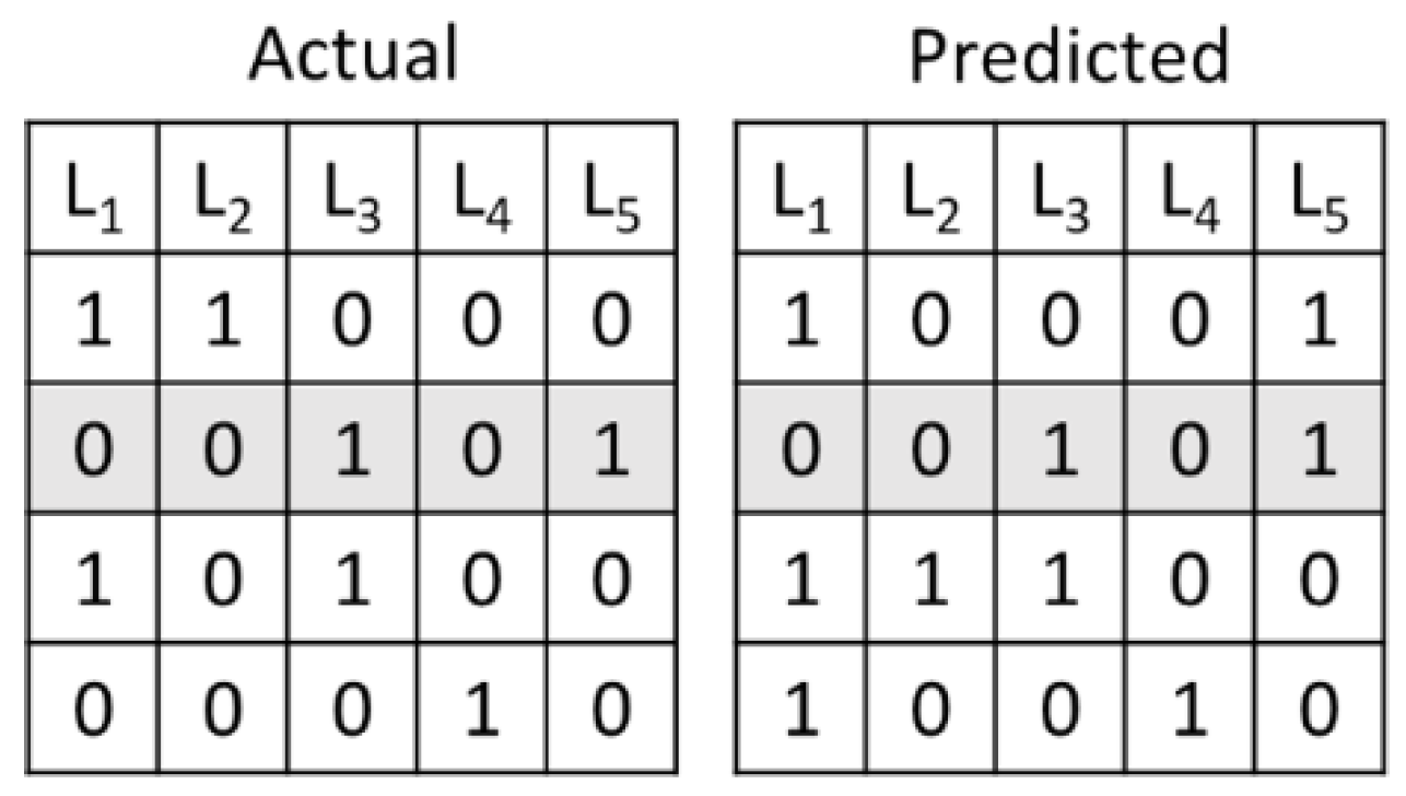
Exact match is also known as subset accuracy (hereinafter abbreviated as Acc.). It is the most rigorous performance indicator and represents the fraction at which the labels of each instance can be correctly classified:
where is the indicator function. Figure 4 illustrates an example of the accuracy of the subset. In this case, the accuracy is calculated to be 1/4.
3. Experimental Analysis
In this study, a series of experiments were conducted to illustrate the benefits of the proposed method. The performance of the proposed method was compared with various traditional classification algorithms.
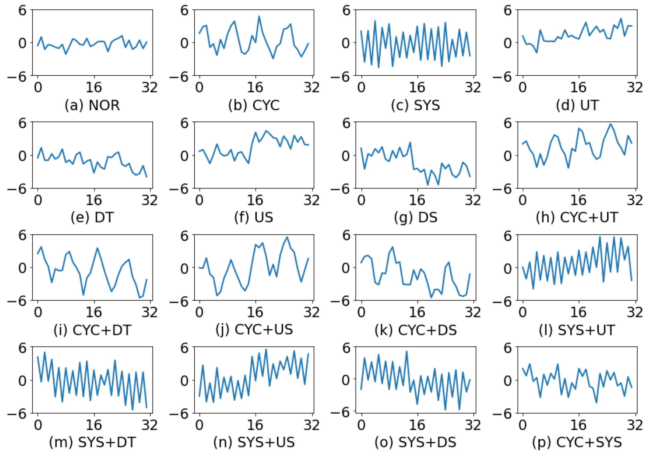
In the first experiment, the data of non-random patterns were generated based on the pattern parameter settings of Hong et al. [24]. They set the analysis window size to 32, and explored 16 patterns, including 7 single patterns and 9 concurrent patterns (Figure 5). In the training set, there were 5000 samples for each pattern, and in the test dataset, there were 1250 samples for each pattern.
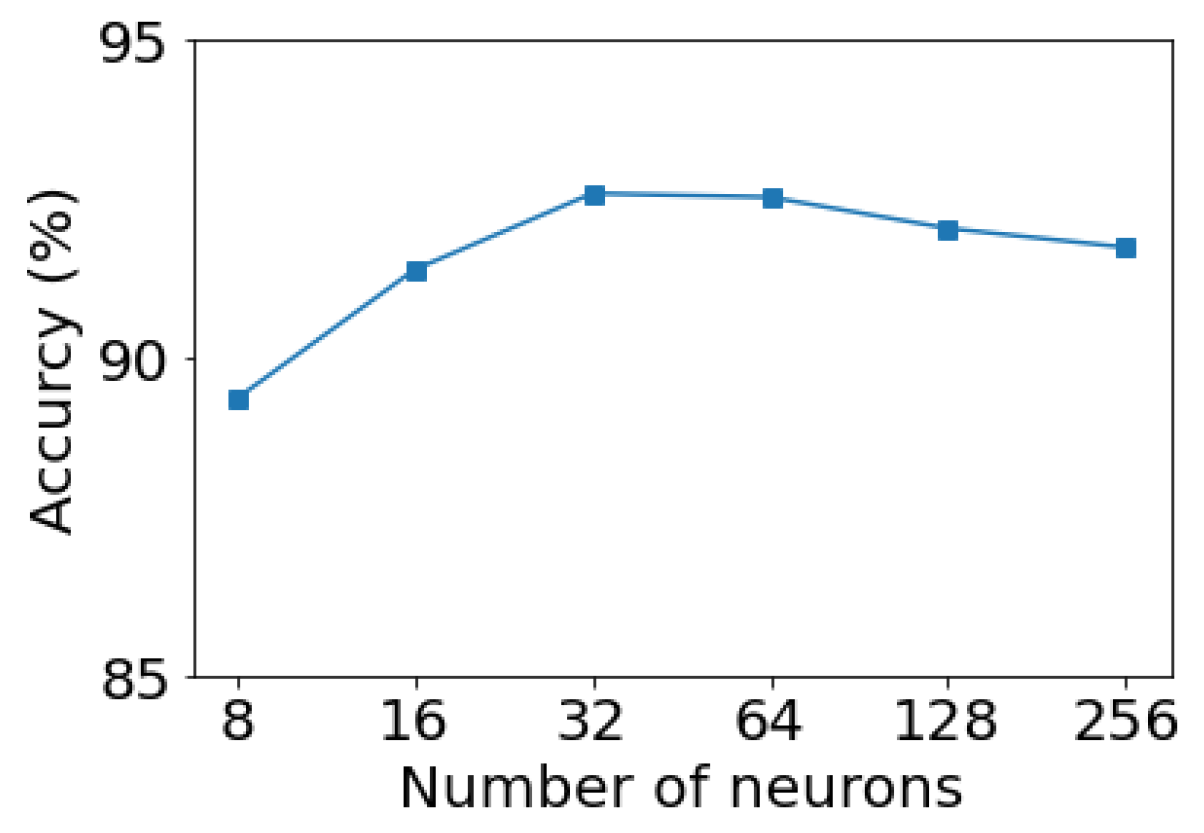
In the present study, Keras [44] was used to build a multi-label convolutional neural network. To identify an optimized 1D CNN architecture, various structural and learning parameters were needed, such as the number of filters in each convolution layer, the filter size, the stride, and the number of neurons in the fully connected layers. The input data were a 1D vector containing 32 observations, and the output layer contained 7 neurons corresponding to 7 single pattern types. Since the amount of data for training was limited, it was not feasible to use deeper architectures without causing significant overfitting. The proposed 1D CNN had two convolution layers. The first convolution layer had 16 filters of size , and the second convolution layer had 32 filters of size . A large filter size was used in the first convolutional layer because it was assumed that the first layer should have a higher-level view of the control chart data. The convolution stride in the network was fixed to 1. The padding type was set to “same” (zero padding) to avoid the loss of spatial dimensions. The size of the max pooling window was with a stride of 2. Dropout was added to each convolution layer to reduce model complexity and prevent overfitting. The proposed end-to-end 1D CNN included one fully connected layer. The fully connected layer had 32 neurons that were chosen after trial and error. Figure 6 illustrates the effect of the number of neurons on accuracy. Dropout was also added to the fully connected layer. The ReLU activation function () was used for all layers, except for the output layer where a sigmoid activation function was used. The CNN architecture is summarized in Table 1.
The Adam optimization algorithm and cross-entropy loss function were used to train the 1D CNN with a batch size of 16. The 1D CNN was trained up to 100 epochs with a learning rate of 0.001. To avoid overfitting, an early stopping procedure was employed; specifically, the loss value of the validation set was monitored in each epoch and the training procedure was halted if training yielded no improvements within the previous 10 epochs.
This study selected RF [49] and SVC [47] as the competing methods, both of which can support multi-label classification problems. In this study, a one-vs-the-rest (OVR) multi-label classifier was established based on SVC. OVR is also called one-vs-all, which is to build a binary classifier for each class. The above-mentioned classifiers were built in Python with scikit-learn v0.24.1 [48].
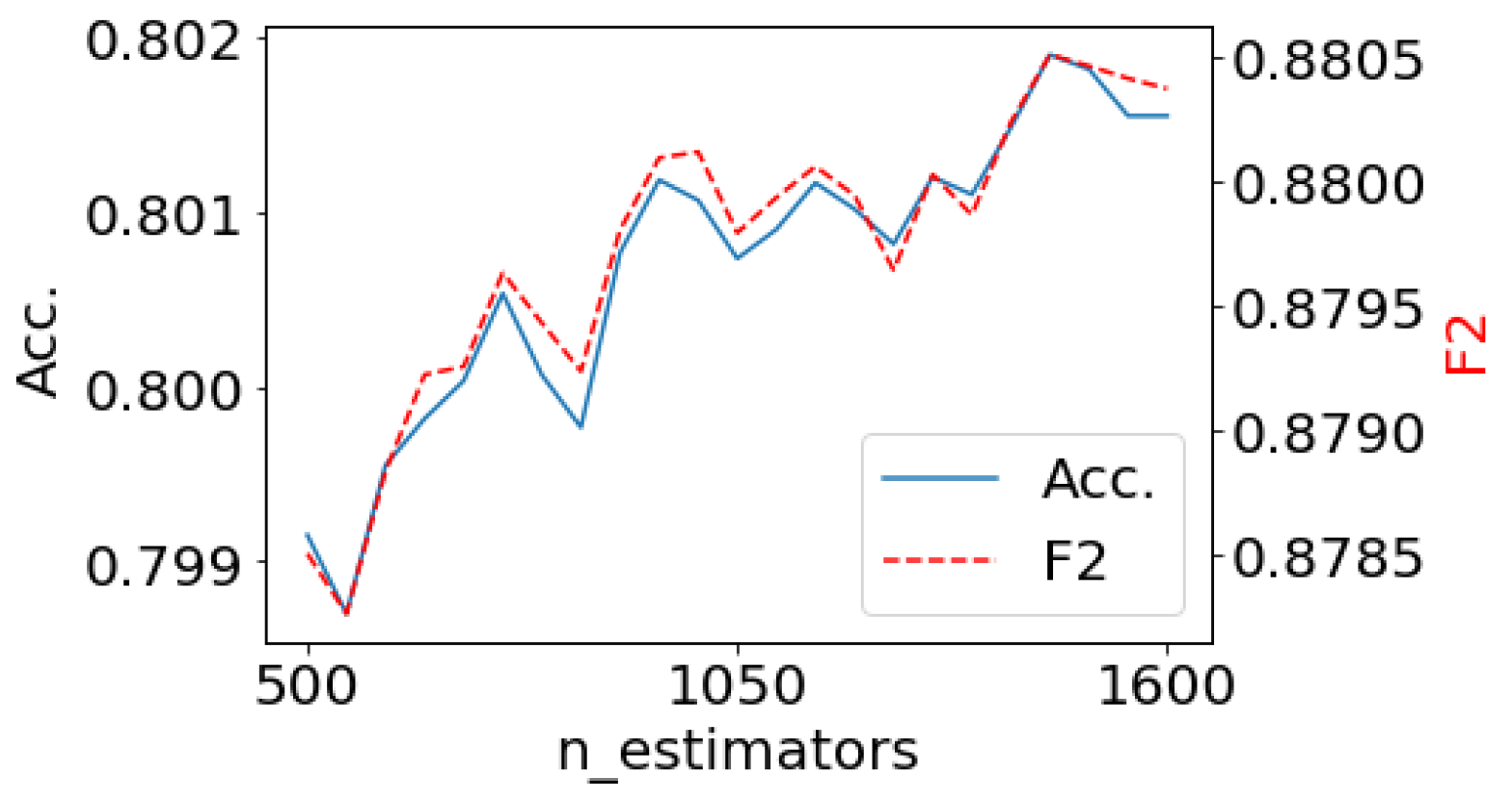
For RF, the maximum depth of each tree was not restricted. The number of features used for each decision split was set to the square root of the total feature number. The number of trees () was identified by evaluating the results for a range of values. Figure 7 illustrates the performance of RF when the number of individual decision trees were varied. From Figure 7, it follows that increasing the number of trees beyond 1450 would result in minor improvement of accuracy. Therefore, 1450 trees were used to reduce the computation time.
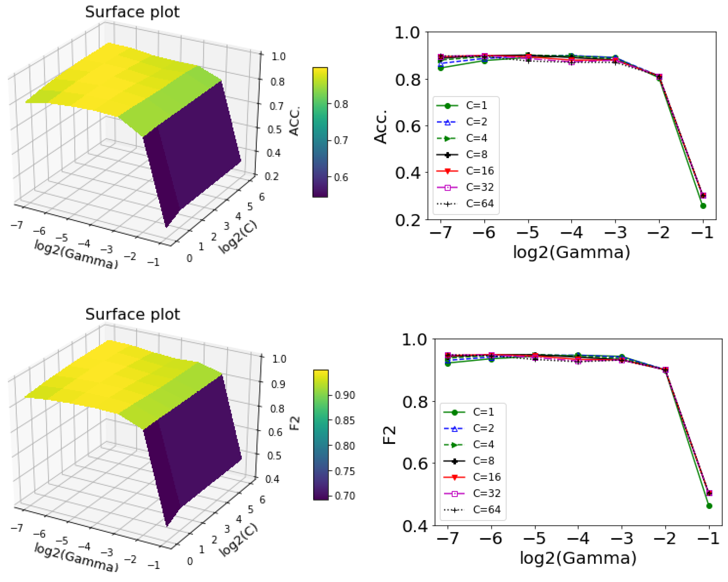
For SVC, this study chose the radial basis function (RBF) as the kernel function. The hyperparameters and of SVC were chosen using the grid search method. Figure 8 illustrates the performance of SVC with different parameter settings. The value had a small effect on the accuracy rate (or score). The best performance of SVC was achieved when the parameters and were set to 4 and 0.03125, respectively. The best value (0.03125) obtained from the grid search was equivalent to 1/the number of input features, which was 1/32.
Because RF and CNN are stochastic, this study took the average of multiple runs (10 times) when evaluating model performance. The randomness of CNN comes from the influence of initial weights. The randomness of RF arises from bootstrap sampling and feature selection. The performance measures are summarized in terms of the mean and standard deviation across all runs. All performance metrics presented hereafter are expressed in decimal form.
Table 2 summarizes the performance of the multi-label CNN classifier and other traditional classifiers. The multi-class CNN developed by Hong et al. [26] achieved an accuracy of 0.9235. The proposed multi-label CNN was the best performing classifier. Of the traditional classifiers evaluated, SVC performed better than RF. The recall rate and precision of RF were somewhat different, but other classifiers had very similar recall rates and precision. When partially correct matches were considered, CNN achieved the lowest Hamming loss (0.0198), indicating its superiority in classification.
The second experiment was based on the work of Zhang and Cheng [51]. The authors developed an SVM-based classifier for CCPR. Six basic patterns and four concurrent patterns were investigated. They set the analysis window size to 40. In the training and test datasets, 50 samples were used for each pattern class and 13 statistical and shape features were used as inputs for the SVM. The SVM was optimized using genetic algorithms. Table 3 summarizes the architecture of the proposed CNN. The training process was similar to that used in the first experiment.
Using the procedure described in experiment 1, the number of trees for RF was 900. SVC used RBF kernel function. After a grid search study, the parameters and were set to 16.0 and , respectively. Table 4 summarizes the classification results for the second experiment. According to the results in Table 4, CNN achieved the highest overall classification accuracy (0.9876), followed by SVC (0.9760) and RF (0.8652). The SVC method used in this study obtained the same classification accuracy as that reported by Zhang and Cheng [51]. The proposed multi-label CNN still performed the best in terms of the other metrics.
Table 5 provides a detailed comparison between the proposed multi-label CNN and the feature-based SVC developed by Zhang and Cheng [51]. It is clear that the proposed multi-label CNN outperformed the feature-based SVC in classifying the concurrent pattern which is composed of cycle, upward trend and downward shift. It seems that multi-label CNN has the advantage of classifying complex concurrent patterns.
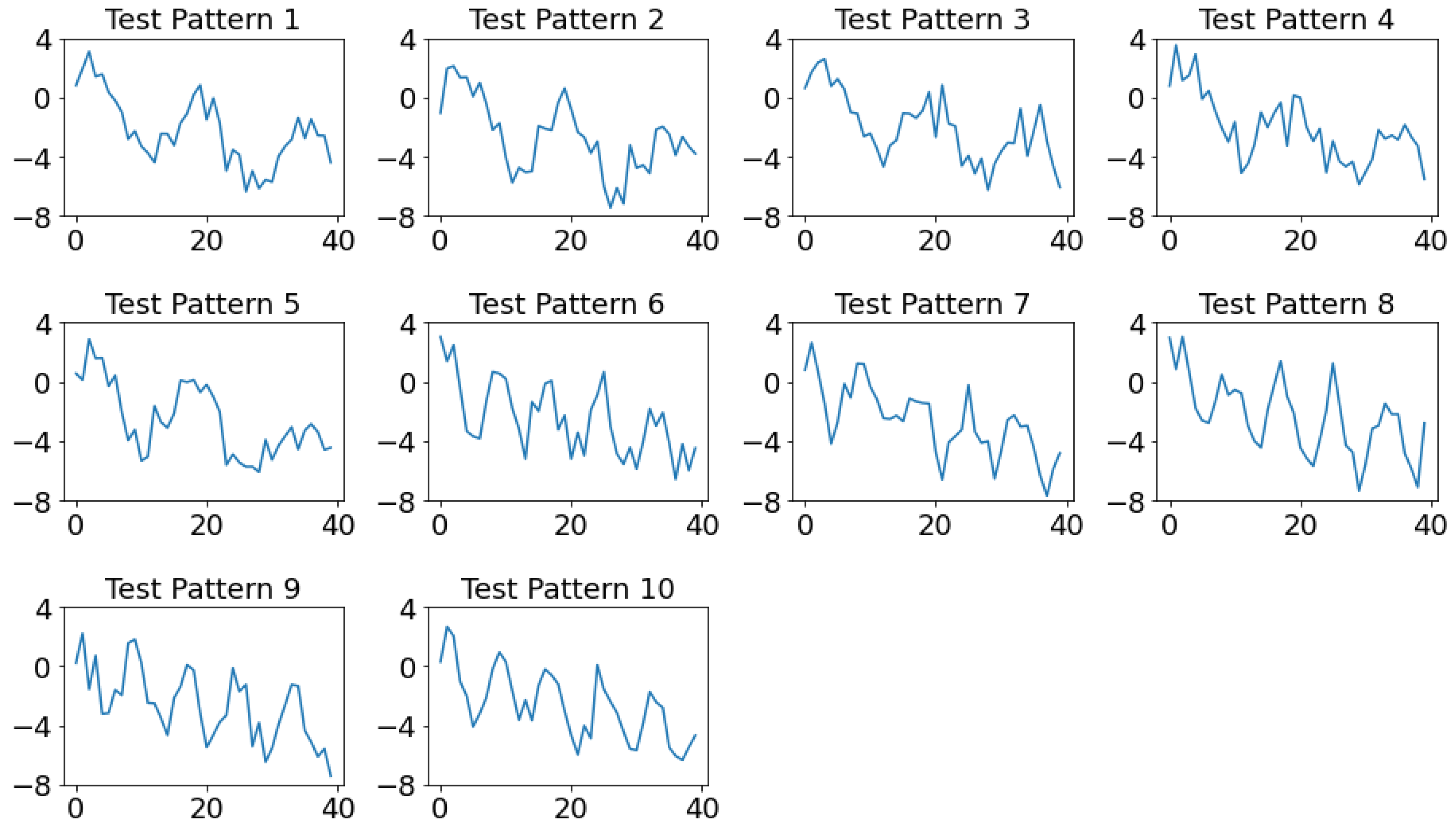
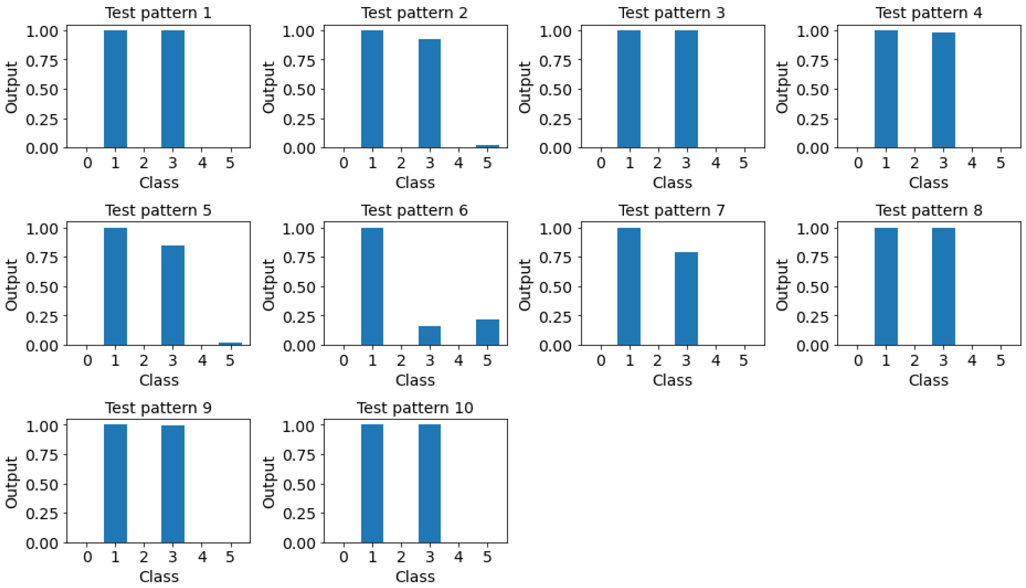
The advantages of using a multi-label classification model instead of a multi-class model for concurrent CCPR can be illustrated with the following example. The original paper [51] only considered a concurrent pattern of cycles and upward trends. Therefore, the concurrent pattern of cycles and downward trends can be considered an unknown pattern. Restricted by the predefined pattern classes of the multi-class model, in the best case, this concurrent pattern can be classified as a class label including the features of either a cycle or a downward trend. In the worst-case scenario, it can be classified as a normal pattern or as some other pattern. Ten additional concurrent patterns that featured a cycle and downward trend were simulated. Figure 9 depicts these 10 concurrent patterns. The results of the multi-label CNN are presented in Figure 10. According to the coding scheme of the original paper, the desired output should be (0,1,0,1,0,0). As evident, only one misclassified pattern was present. Pattern six was misclassified as a single cyclic pattern. As can be seen in Figure 10, only the neuron corresponding to the cycle was fired. That is, the output value was greater than the default threshold value of 0.5. As expected, the traditional classifiers misclassified all 10 patterns. For RF, three patterns were classified as a single downward trend and seven patterns were classified as concurrent patterns involving a cycle and a downward shift. For SVC, all 10 patterns were misclassified as concurrent patterns involving a cycle and a downward shift. These results indicate that the multi-class classification models can, at best, select a class label that most resembles the unseen input pattern as the output. This example demonstrates the benefits of using multi-label CNN in control chart concurrent pattern recognition.
The third experiment addressed cases in which the basic constituents of concurrent patterns may have different change points (cases in which multiple non-random patterns do not appear at the same time). Little research has been conducted on such cases [24,32]. Zhang and Cheng [51] set the change point of the non-random patterns to a fixed point in time. The shift position () of shift patterns was set to be 2; shift patterns were present when and other non-random patterns started from . In the present experiment, shifts can occur at different locations in the window. The shift position was set to . With this setting, a concurrent pattern that involves a shift may have different change points.
Table 6 summarizes the results of each classification model. The hyperparameters and the training process were similar to those used in the second experiment. A comparison of the results in Table 4 and Table 6 reveals that the performance of traditional classifiers decreased dramatically. It can be seen from the table that CNN’s classification accuracy and other performance metrics were better than those of traditional classifiers. What makes CNN different from other classification algorithms is its translation invariance property. The results demonstrate that CNN maintains high accuracy when basic constituents of concurrent patterns may not appear at the same point in time.
The final experiment explored a more rigorous evaluation of the proposed method using a different setting of in the training set and the test set. For the training dataset, the shift position was ; for the test dataset, it was . By manipulating the shift position , the non-random patterns encountered in the test stage can differ from those learned in the training stage. The hyperparameters and the training process were determined using the same method as that used in the second experiment. Table 7 summarizes the results of each classification model. A degradation of performance for all classifiers can be observed. Performance degradation might be due to the setting of the shift position . Different settings for creates variants that are not seen in the training stage. As evident in Table 7, CNN still performed the best among the classifiers that were compared. To extent the analysis, this study swapped the training and testing sets. As indicated in Table 8, CNN outperformed other classifiers in all evaluation metrics. This experiment reveals that CNN is much more resilient against the variation in change points of the basic constituents of concurrent patterns. RF performed the worst out of all the methods. This is because RF takes raw data as inputs and each observation is treated as an individual feature. This makes RF very sensitive to the location of features.
4. Illustrative Example
In this section, the application of online monitoring is illustrated with the data collected from a cleaning process in integrated circuit (IC) carrier production. The process quality characteristic of interest is the concentration of a sodium carbonate solution. The manufacturer applied an individual and moving range chart (- Chart) with supplementary rules [2,3,4] to monitor the concentration of the solutions. The chemical concentration exhibited abnormal variations that might be due to multiple assignable causes: variation in the initial bath make-up, mistakes in dose calculations, an incorrect dosing formula, irregular manual dosing operations, or the malfunction of the automatic dosing system. Irregular demand can also induce abnormal variation in the concentration. The assignable causes in this example made the data to show periodic changes and downward trends.
To implement the proposed method, the moving/sliding window size was set to 32. At each step, the window advances to include a new observation and discard an old one. The multi-label CNN model developed in experiment 1 was applied to this monitoring task. In the illustration shown below, only parts of the windows are used to display the results of online monitoring.
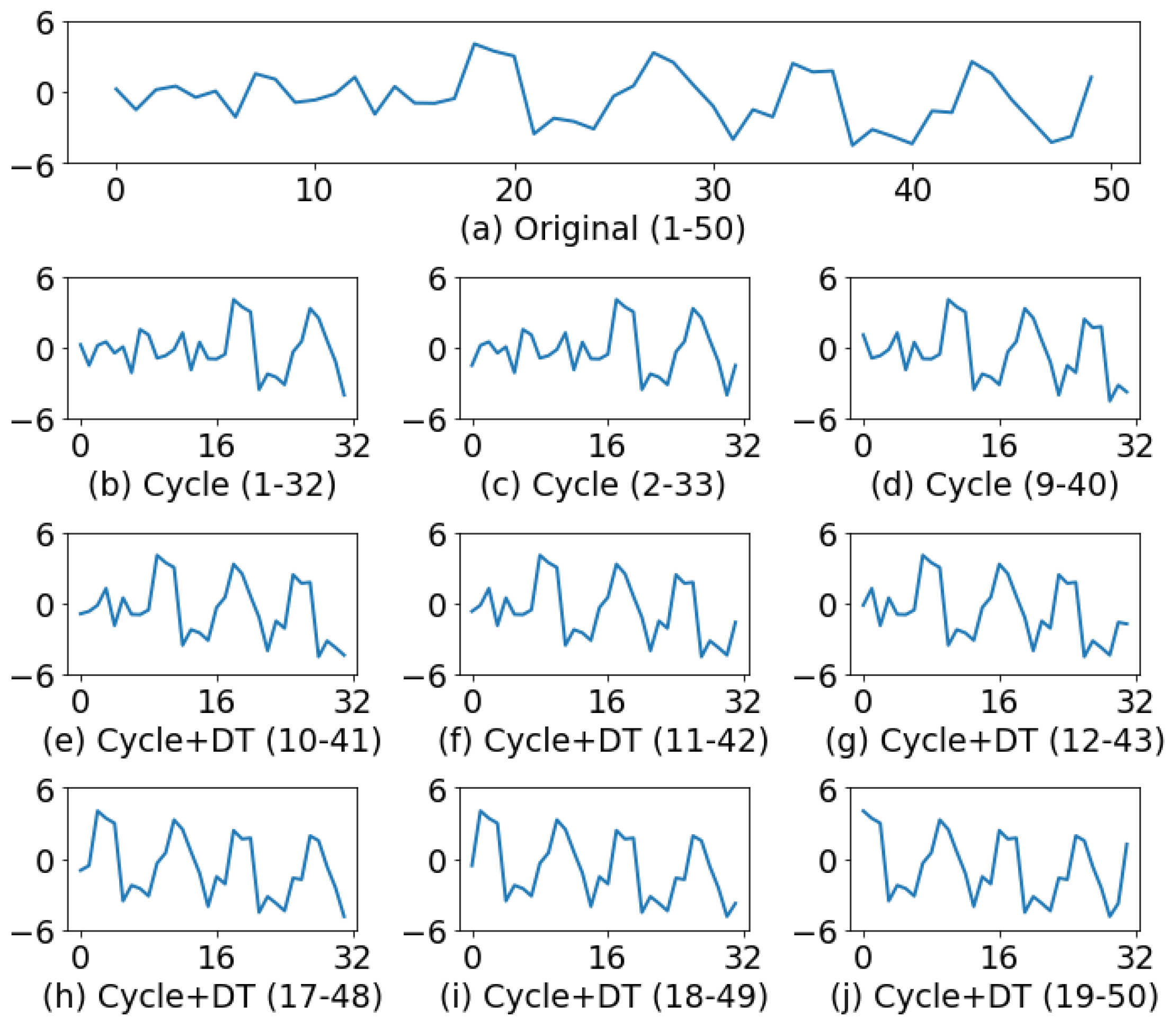
Figure 11a shows the 50 observations collected, all of which were standardized to have zero mean and unit variance. The process began to exhibit a cyclic pattern and downward trend from the 19th observation onward. Figure 11b is the first analysis window. Although the number of cyclic pattern data only accounts for 44% (14/32) of the window size, the CNN classifier can still correctly identify periodic changes. If the assignable cause for the periodic changes can be correctly diagnosed and eliminated, the cyclical variation will be no longer present. In case that the assignable causes cannot be eliminated, the downward trend will become more noticeable as more data are collected from the process. Starting from the 10th analysis window (Figure 11e), the identification results of the CNN model are a cyclic pattern and downward trend. Figure 11j shows the complete concurrent pattern data. It is evident from this figure that the non-random patterns shown in the process data are cyclic and downward trend.
5. Conclusions
In this study, a multi-label classification method was developed using CNN architectures to classify control chart concurrent patterns. A series of experiments were conducted using datasets from previous studies to evaluate the performance of the proposed method. The results reveal that a multi-label CNN performed better than other multi-label classifiers that were compared. The superior performance of a multi-label CNN can be partly explained by its translation invariance property. This feature allows CNN to maintain high accuracy when basic constituents of concurrent patterns may not appear at the same point in time. The traditional classifiers take raw data as inputs and each observation is treated as an individual feature. This makes traditional classifiers very sensitive to the location of features. This study also used a set of industry data to illustrate the applicability of the proposed CNN to online monitoring. The results reveal that the proposed multi-label CNN can be applied to online monitoring and can correctly identify concurrent patterns. The results reveal that that multi-label CNN has the potential to classify concurrent control chart patterns. The results of this study contribute to the further realization of smart SPC.
This study has several limitations that can be addressed in future research. First, the proposed multi-label CNN was compared with traditional classifiers that used raw data as inputs. In future work, it is worth evaluating the traditional multi-label classifiers using features as inputs. Second, this study considered the case when the constituents of the concurrent pattern may not appear at the same time. In practical application, the change positions of each individual patterns may be more complicated than those considered in this study. Future research should investigate more sophisticated situations when non-random patterns may have different change points and change magnitudes. Finally, this study applied a single threshold to all labels. Future research should consider applying thresholding techniques, such as multi-thresholds, to improve the performance of multi-label classification.
Author Contributions
Conceptualization, C.-S.C.; Methodology, C.-S.C.; Software, C.-S.C. and P.-W.C.; Formal analysis, C.-S.C., P.-W.C. and Y.H.; Investigation, C.-S.C. and P.-W.C.; Data curation, P.-W.C. and Y.H; Writing-Original Draft Preparation, C.-S.C., P.-W.C. and Y.H.; Writing-Review and Editing, C.-S.C.; Supervision, C.-S.C. All authors have read and agreed to the published version of the manuscript.
Funding
This research was partially funded by the Ministry of Science and Technology, R.O.C. (grant number 109-2221-E-155-020-).
Institutional Review Board Statement
Not applicable.
Informed Consent Statement
Not applicable.
Data Availability Statement
The simulated datasets used in this study are available from the corresponding author on reasonable request.
Conflicts of Interest
The authors declare no conflict of interest.
References
- Montgomery, D.C. Introduction to Statistical Quality Control, 8th ed.; John Wiley & Sons: New York, NY, USA, 2020. [Google Scholar]
- Western Electric. Statistical Quality Control Handbook; Western Electric Company: Indianapolis, IN, USA, 1956. [Google Scholar]
- Nelson, L.S. The Shewhart control chart tests for special causes. J. Qual. Technol. 1984, 16, 237–239. [Google Scholar] [CrossRef]
- Nelson, L.S. Interpreting Shewhart control chart. J. Qual. Technol. 1985, 17, 114–116. [Google Scholar] [CrossRef]
- Cheng, C.S. A neural network approach for the analysis of control chart patterns. Int. J. Prod. Res. 1997, 35, 667–697. [Google Scholar] [CrossRef]
- Evans, J.R.; Lindsay, W.M. A framework for expert system development in statistical quality control. Comput. Ind. Eng. 1988, 14, 335–343. [Google Scholar] [CrossRef]
- Swift, J.A.; Mize, J.H. Out-of-control pattern recognition and analysis for quality control charts using LISP-based systems. Comput. Ind. Eng. 1995, 28, 81–91. [Google Scholar] [CrossRef]
- Guh, R.S. Optimizing feed forward neural networks for control chart pattern recognition through genetic algorithms. Int. J. Pattern Recognit. Artif. Intell. 2004, 18, 75–99. [Google Scholar] [CrossRef]
- Zorriassatine, F.; Tannock, J.D.T. A review of neural networks for statistical process control. J. Intell. Manuf. 1998, 9, 209–224. [Google Scholar] [CrossRef]
- Perry, M.; Pignatiello, J. A review of artificial neural network applications in control chart pattern recognition. In Proceedings of the Industrial Engineering Research Conference, Orlando, FL, USA, 21–25 May 2002. [Google Scholar]
- Barghash, M.A. Literature survey on pattern recognition in control charts using artificial neural networks. In Proceedings of the 37th International Conference on Computers and Industrial Engineering, Alexandria, Egypt, 20–23 October 2007; pp. 1870–1880. [Google Scholar]
- Hachicha, W.; Ghorbel, A. A survey of control chart pattern recognition literature (1991–2010) based on a new conceptual classification scheme. Comput. Ind. Eng. 2012, 63, 204–222. [Google Scholar] [CrossRef]
- Gauri, S.K.; Chakraborty, S. Recognition of control chart patterns using improved selection of features. Comput. Ind. Eng. 2009, 56, 1577–1588. [Google Scholar] [CrossRef]
- Ranaee, V.; Ebrahimzadeh, A. Control chart pattern recognition using neural networks and efficient features: A comparative study. Pattern Anal. Appl. 2013, 16, 321–332. [Google Scholar] [CrossRef]
- Addeh, A.; Khormali, A.; Golilarz, N.A. Control chart pattern recognition using RBF neural network with new training algorithm and practical features. ISA Trans. 2018, 79, 202–216. [Google Scholar] [CrossRef]
- Ranaee, V.; Ebrahimzadeh, A. Control chart pattern recognition using a novel hybrid intelligent method. Appl. Soft Comput. 2011, 11, 2676–2686. [Google Scholar] [CrossRef]
- Hassan, A.; Baksh, M.S.N.; Shaharoun, A.M.; Jamaluddin, H. Improved SPC chart pattern recognition using statistical features. Int. J. Prod. Res. 2003, 41, 1587–1603. [Google Scholar] [CrossRef]
- Pham, D.T.; Wani, M.A. Feature-based control chart pattern recognition. Int. J. Prod. Res. 1997, 35, 1875–1890. [Google Scholar] [CrossRef]
- Bag, M.; Gauri, S.K.; Chakraborty, S. An expert system for control chart pattern recognition. Int. J. Adv. Manuf. Syst. 2012, 62, 291–301. [Google Scholar] [CrossRef]
- Pham, D.T.; Oztemel, E. Control chart pattern recognition using neural networks. J. Syst. Eng. Electron. 1992, 2, 256–262. [Google Scholar]
- Guh, R.S.; Tannock, J.D.T. Recognition of control chart concurrent patterns using a neural network approach. Int. J. Prod. Res. 1999, 37, 1743–1765. [Google Scholar] [CrossRef]
- Ranaee, V.; Ebrahimzadeh, A.; Ghaderi, R. Application of the PSO-SVM model for recognition of control chart patterns. ISA Trans. 2010, 49, 577–586. [Google Scholar] [CrossRef] [PubMed]
- Zhang, M.; Yuan, Y.; Wang, R.; Cheng, W. Recognition of mixture control chart patterns based on fusion feature reduction and fireworks algorithm-optimized MSVM. Pattern Anal. Appl. 2020, 23, 15–26. [Google Scholar] [CrossRef]
- Hong, Z.; Li, Y.; Zeng, Z. Convolutional neural network for control chart patterns recognition. In Proceedings of the CSAE 2019: 3rd International Conference on Computer Science and Application Engineering, Sanya, China, 22–24 October 2019. [Google Scholar]
- Miao, Z.; Yang, M. Control chart pattern recognition based on convolution neural network. In Smart Innovations in Communication and Computational Sciences, Advances in Intelligent Systems and Computing (AISC), 670; Panigrahi, B., Trivedi, M., Mishra, K., Tiwari, S., Singh, P., Eds.; Springer: Singapore, 2019; pp. 97–104. [Google Scholar]
- Zan, T.; Liu, Z.; Su, Z.; Wang, M.; Gao, X.; Chen, D. Statistical process control with intelligence based on the deep learning model. Appl. Sci. 2020, 10, 308. [Google Scholar] [CrossRef] [Green Version]
- Cheng, C.S.; Ho, Y.; Chiu, T.C. End-to-end control chart pattern classification using a 1D convolutional neural network and transfer learning. Processes 2021, 9, 1484. [Google Scholar] [CrossRef]
- Zan, T.; Liu, Z.; Wang, H.; Wang, M.; Gao, X. Control chart pattern recognition using the convolutional neural network. J. Intell. Manuf. 2020, 31, 703–716. [Google Scholar] [CrossRef]
- Chen, Z.; Lu, S.; Lam, S. A hybrid system for SPC concurrent pattern recognition. Adv. Eng. Inform. 2007, 21, 303–310. [Google Scholar] [CrossRef]
- Yang, W.A.; Zhou, W.; Liao, W.; Gou, Y. Identification and quantification of concurrent control chart patterns using extreme-point symmetric mode decomposition and extreme learning machines. Neurocomputing 2015, 147, 260–270. [Google Scholar] [CrossRef]
- Shao, Y.E.; Chang, P.Y. Classification of the mixture disturbance patterns for a manufacturing process. J. Ind. Intell. Inf. 2016, 4, 252–256. [Google Scholar] [CrossRef] [Green Version]
- Al-Assaf, Y. Multi-resolution wavelets analysis approach for the recognition of concurrent control chart patterns. Qual. Eng. 2005, 17, 11–21. [Google Scholar] [CrossRef]
- Du, S.; Huang, D.; Lv, J. Recognition of concurrent control chart patterns using wavelet transform decomposition and multiclass support vector machines. Comput. Ind. Eng. 2013, 66, 683–695. [Google Scholar] [CrossRef]
- Wang, C.; Dong, T.; Kuo, W. A hybrid approach for identification of concurrent control chart patterns. J. Intell. Manuf. 2009, 20, 409–419. [Google Scholar] [CrossRef]
- Gu, N.; Cao, Z.; Xie, L.; Creighton, D.; Tan, M.; Nahavandi, S. Identification of concurrent control chart patterns with singular spectrum analysis and learning vector quantization. J. Intell. Manuf. 2013, 24, 1241–1252. [Google Scholar] [CrossRef]
- Xie, L.; Gu, N.; Li, D.; Cao, Z.; Tan, M.; Nahavandi, S. Concurrent control chart patterns recognition with singular spectrum analysis and support vector machine. Comput. Ind. Eng. 2013, 64, 280–289. [Google Scholar] [CrossRef]
- Al-Saffar, A.A.M.; Tao, H.; Talab, M.A. Review of deep convolution neural network in image classification. In Proceedings of the 2017 International Conference on Radar, Antenna, Microwave, Electronics, and Telecommunications (ICRAMET), Jakarta, Indonesia, 23–24 October 2017; Institute of Electrical and Electronics Engineers (IEEE): Piscataway, NJ, USA, 2017. [Google Scholar]
- Aloysius, N.; Geetha, M. A review on deep convolutional neural networks. In Proceedings of the 2017 International Conference on Communication and Signal Processing (ICCSP), Chennai, India, 6–8 April 2017; Institute of Electrical and Electronics Engineers (IEEE): Piscataway, NJ, USA, 2017. [Google Scholar]
- Ajit, A.; Acharya, K.; Samanta, A. A review of convolutional neural networks. In Proceedings of the 2020 International Conference on Emerging Trends in Information Technology and Engineering (IC-ETITE), Vellore, India, 24–25 February 2020; Institute of Electrical and Electronics Engineers (IEEE): Piscataway, NJ, USA, 2020. [Google Scholar]
- Fawaz, H.I.; Forestier, G.; Weber, J.; Idoumghar, L.; Muller, P.A. Deep learning for time series classification: A review. Data Min. Knowl. Discov. 2019, 33, 917–963. [Google Scholar] [CrossRef] [Green Version]
- Kiranyaz, S.; Avci, O.; Abdeljaber, O.; Ince, T.; Gabbouj, M.; Inman, D.J. 1D convolutional neural networks and applications: A survey. Mech. Syst. Signal Process 2021, 151, 107398. [Google Scholar] [CrossRef]
- Shorten, C.; Khoshgoftaar, T.M. A survey on image data augmentation for deep learning. J. Big Data 2019, 6, 60. [Google Scholar] [CrossRef]
- Du, W.; Wang, S.; Gong, X.; Wang, H.; Yao, X.; Pecht, M. Translation invariance-based deep learning for rotating machinery diagnosis. Shock Vib. 2020, 2020, 1635621. [Google Scholar] [CrossRef]
- Chollet, F. Keras. 2015. Available online: https://github.com/fchollet/keras (accessed on 14 December 2021).
- Yamashita, R.; Nishio, M.; Do, R.K.G.; Togashi, K. Convolutional neural networks: An overview and application in radiology. Insights Imaging 2018, 9, 611–629. [Google Scholar] [CrossRef] [PubMed] [Green Version]
- Gibaja, E.; Ventura, S. A tutorial on multi-label learning. ACM Comput. Surv. 2015, 47, 1–38. [Google Scholar] [CrossRef]
- Vapnik, V.N. The Nature of Statistical Learning Theory; Springer: New York, NY, USA, 1995. [Google Scholar]
- Pedregosa, F.; Varoquaux, G.; Gramfort, A.; Michel, V.; Thirion, B.; Grisel, O.; Blondel, M.; Prettenhofer, P.; Weiss, R.; Dubourg, V.; et al. Scikit-learn: Machine Learning in Python. J. Mach. Learn. Res. 2011, 12, 2825–2830. [Google Scholar]
- Breiman, L. Random forests. Mach. Learn. 2001, 45, 5–32. [Google Scholar] [CrossRef] [Green Version]
- Wu, X.Z.; Zhou, Z.H. A unified view of multi-label performance measures. In Proceedings of the 24th International Conference on Machine Learning and Computing, Corvallis, OR, USA, 20–24 June 2007; pp. 3780–3788. [Google Scholar]
- Zhang, M.; Cheng, W. Recognition of mixture control chart pattern using multiclass support vector machine and genetic algorithm based on statistical and shape features. Math. Probl. Eng. 2015, 2015, 1–10. [Google Scholar]
Figure 1.
Typical examples of control chart patterns.

Figure 2.
Typical convolutional neural network architecture.

Figure 3.
Example of Hamming loss.

Figure 4.
Example of subset accuracy.

Figure 5.
Single and concurrent patterns.

Figure 6.
Effect of the number of neurons on convolutional neural network performance.

Figure 7.
Effect of the number of decision trees on random forest performance.

Figure 8.
Effect of parameters on support vector classification performance.

Figure 9.
Test patterns for experiment 2.

Figure 10.
The results of the multi-label 1D CNN.

Figure 11.
Application of online monitoring.


Table 1.
Convolutional neural network architecture for experiment 1.
| Layer | Type | Filter Size | #Filters | Stride | Padding |
|---|---|---|---|---|---|
| 1 | Convolution/ReLU | 16 | 1 | same | |
| 2 | Max pooling | 1 | 2 | - | |
| 3 | Dropout (10%) | - | - | - | - |
| 4 | Convolution/ReLU | 32 | 1 | same | |
| 5 | Max pooling | 1 | 2 | - | |
| 6 | Dropout (10%) | - | - | - | - |
| 7 | Fully connected (32) | - | - | - | - |
| 8 | Dropout (10%) | - | - | - | - |
| 9 | Sigmoid (7) | - | - | - | - |
Table 2.
Classification performance in experiment 1.
| Metric\Algorithm | RF | SVC | CNN |
|---|---|---|---|
| Accuracy | 0.8019 (0.0023) * | 0.9008 | 0.9256 (0.0003) |
| Recall | 0.8752 (0.0019) | 0.9508 | 0.9563 (0.0005) |
| Precision | 0.9228 (0.0019) | 0.9521 | 0.9588 (0.0006) |
| 0.8910 (0.0019) | 0.9491 | 0.9568 (0.0004) | |
| 0.8805 (0.0019) | 0.9496 | 0.9563 (0.0005) | |
| Hamming loss | 0.0383 (0.0005) | 0.0228 | 0.0198 (0.0001) |
| Jaccard_score | 0.8355 (0.0019) | 0.9027 | 0.9150 (0.0005) |
*: Numbers in parentheses are standard deviations.
Table 3.
Convolutional neural network architecture for experiment 2.
| Layer | Type | Filter Size | #Filters | Stride | Padding |
|---|---|---|---|---|---|
| 1 | Convolution/ReLU | 32 | 1 | same | |
| 2 | Max pooling | 1 | 2 | - | |
| 3 | Convolution/ReLU | 128 | 1 | same | |
| 4 | Max pooling | 1 | 2 | - | |
| 5 | Dropout (30%) | - | - | - | - |
| 6 | Convolution/ReLU | 256 | 1 | same | |
| 7 | Max pooling | 1 | 2 | - | |
| 8 | Dropout (30%) | - | - | - | - |
| 9 | Fully connected (128) | - | - | - | - |
| 10 | Dropout (30%) | - | - | - | - |
| 11 | Sigmoid (6) | - | - | - | - |
Table 4.
Classification performance in experiment 2.
| Metric\Algorithm | RF | SVC | CNN |
|---|---|---|---|
| Accuracy | 0.8652 (0.0034) * | 0.9760 | 0.9876 (0.0016) |
| Recall | 0.8888 (0.0030) | 0.9877 | 0.9930 (0.0016) |
| Precision | 0.9073 (0.0039) | 0.9910 | 0.9937 (0.0018) |
| 0.8953 (0.0032) | 0.9882 | 0.9927 (0.0011) | |
| 0.8910 (0.0031) | 0.9876 | 0.9927 (0.0012) | |
| Hamming loss | 0.0232 (0.0007) | 0.0047 | 0.0032 (0.0008) |
| Jaccard_score | 0.9073 (0.0028) | 0.9814 | 0.9917 (0.0008) |
*: Numbers in parentheses are standard deviations.
Table 5.
A detailed comparison between the proposed multi-label CNN and the feature-based SVC developed by Zhang and Cheng [51].
Table 5.
A detailed comparison between the proposed multi-label CNN and the feature-based SVC developed by Zhang and Cheng [51].
| Zhang and Cheng [51] | This Work | ||
|---|---|---|---|
| Pattern | Accuracy | Label | Accuracy |
| NOR | 1.0 | (1,0,0,0,0,0) | 1.0 |
| CYC | 0.98 | (0,1,0,0,0,0) | 1.0 |
| UT | 0.98 | (0,0,1,0,0,0) | 1.0 |
| DT | 1.0 | (0,0,0,1,0,0) | 1.0 |
| US | 1.0 | (0,0,0,0,1,0) | 0.98 |
| DS | 0.98 | (0,0,0,0,0,1) | 0.98 |
| CYC+UT | 0.98 | (0,1,1,0,0,0) | 1.0 |
| CYC+DS | 1.0 | (0,1,0,0,0,1) | 0.98 |
| UT+DS | 0.96 | (0,0,1,0,0,1) | 0.98 |
| CYC+UT+DS | 0.88 | (0,1,1,0,0,1) | 0.96 |
Table 6.
Classification performance in experiment 3.
| Metric\Algorithm | RF | SVC | CNN |
|---|---|---|---|
| Accuracy | 0.7652 (0.0039) * | 0.9100 | 0.9406 (0.0031) |
| Recall | 0.7945 (0.0026) | 0.9273 | 0.9557 (0.0043) |
| Precision | 0.8131 (0.0031) | 0.9287 | 0.9546 (0.0041) |
| 0.8005 (0.0029) | 0.9259 | 0.9539 (0.0037) | |
| 0.7964 (0.0027) | 0.9262 | 0.9546 (0.0039) | |
| Hamming loss | 0.0481 (0.0011) | 0.0210 | 0.0159 (0.0013) |
| Jaccard_score | 0.8143 (0.0036) | 0.9185 | 0.9383 (0.0050) |
*: Numbers in parentheses are standard deviations.
Table 7.
Classification performance in experiment 4.
| Metric\Algorithm | RF | SVC | CNN |
|---|---|---|---|
| Accuracy | 0.7186 (0.0046) * | 0.8480 | 0.8704 (0.0053) |
| Recall | 0.7448 (0.0040) | 0.8597 | 0.8823 (0.0049) |
| Precision | 0.7612 (0.0046) | 0.8597 | 0.8841 (0.0038) |
| 0.7501 (0.0043) | 0.8585 | 0.8823 (0.0041) | |
| 0.7464 (0.0041) | 0.8588 | 0.8820 (0.0045) | |
| Hamming loss | 0.0632 (0.0008) | 0.0437 | 0.0401 (0.0017) |
| Jaccard_score | 0.7628 (0.0029) | 0.8379 | 0.8509 (0.0057) |
*: Numbers in parentheses are standard deviations.
Table 8.
Classification performance in experiment 4 after swapping the training and test sets.
| Metric\Algorithm | RF | SVC | CNN |
|---|---|---|---|
| Accuracy | 0.7574 (0.0058) * | 0.8640 | 0.9232 (0.0019) |
| Recall | 0.7981 (0.0049) | 0.9110 | 0.9564 (0.0050) |
| Precision | 0.8112 (0.0049) | 0.8960 | 0.9461 (0.0025) |
| 0.7997 (0.0050) | 0.8994 | 0.9486 (0.0032) | |
| 0.7977 (0.0049) | 0.9049 | 0.9523 (0.0041) | |
| Hamming loss | 0.0509 (0.0016) | 0.0307 | 0.0175 (0.0008) |
| Jaccard_score | 0.8052 (0.0055) | 0.8840 | 0.9324 (0.0029) |
*: Numbers in parentheses are standard deviations.
Publisher’s Note: MDPI stays neutral with regard to jurisdictional claims in published maps and institutional affiliations. |
© 2022 by the authors. Licensee MDPI, Basel, Switzerland. This article is an open access article distributed under the terms and conditions of the Creative Commons Attribution (CC BY) license (https://creativecommons.org/licenses/by/4.0/).
Share and Cite
MDPI and ACS Style
Cheng, C.-S.; Chen, P.-W.; Ho, Y. Control Chart Concurrent Pattern Classification Using Multi-Label Convolutional Neural Networks. Appl. Sci. 2022, 12, 787. https://0-doi-org.brum.beds.ac.uk/10.3390/app12020787
AMA Style
Cheng C-S, Chen P-W, Ho Y. Control Chart Concurrent Pattern Classification Using Multi-Label Convolutional Neural Networks. Applied Sciences. 2022; 12(2):787. https://0-doi-org.brum.beds.ac.uk/10.3390/app12020787
Chicago/Turabian StyleCheng, Chuen-Sheng, Pei-Wen Chen, and Ying Ho. 2022. "Control Chart Concurrent Pattern Classification Using Multi-Label Convolutional Neural Networks" Applied Sciences 12, no. 2: 787. https://0-doi-org.brum.beds.ac.uk/10.3390/app12020787
Note that from the first issue of 2016, this journal uses article numbers instead of page numbers. See further details here.