
Comparative Study of Machine Learning Classifiers for Modelling Road Traffic Accidents


1
Department of Applied Information Systems, University of Johannesburg, Johannesburg 2006, South Africa
2
Institute for Intelligent Systems, University of Johannesburg, Johannesburg 2006, South Africa
*
Author to whom correspondence should be addressed.
Appl. Sci. 2022, 12(2), 828; https://0-doi-org.brum.beds.ac.uk/10.3390/app12020828
Submission received: 27 November 2021
/
Revised: 5 January 2022
/
Accepted: 10 January 2022
/
Published: 14 January 2022
(This article belongs to the Special Issue Applied Machine Learning Ⅱ)
Abstract
:Road traffic accidents (RTAs) are a major cause of injuries and fatalities worldwide. In recent years, there has been a growing global interest in analysing RTAs, specifically concerned with analysing and modelling accident data to better understand and assess the causes and effects of accidents. This study analysed the performance of widely used machine learning classifiers using a real-life RTA dataset from Gauteng, South Africa. The study aimed to assess prediction model designs for RTAs to assist transport authorities and policymakers. It considered classifiers such as naïve Bayes, logistic regression, k-nearest neighbour, AdaBoost, support vector machine, random forest, and five missing data methods. These classifiers were evaluated using five evaluation metrics: accuracy, root-mean-square error, precision, recall, and receiver operating characteristic curves. Furthermore, the assessment involved parameter adjustment and incorporated dimensionality reduction techniques. The empirical results and analyses show that the RF classifier, combined with multiple imputations by chained equations, yielded the best performance when compared with the other combinations.
1. Introduction
The rapidly increasing number of road traffic accidents (RTAs) has negatively affected different countries by resulting in a high number of injuries and fatalities. The World Economic Forum [1] estimates that the number of vehicles worldwide is expected to double by 2040, putting more pressure on the transport infrastructure. According to the World Health Organisation (WHO) [2,3], RTAs are likely to be the seventh leading cause of death by 2030. The WHO further stipulated that RTAs cause death to vulnerable road users because more than half (54%) of the individuals killed on the roads are cyclists, motorcyclists, and pedestrians. An RTA can be described as an accident that occurs when at least one road vehicle is involved in an accident which happens on an open public road, and at least one person ends up being killed or injured [4]. The leading recorded causes of RTAs are speeding, driving under the influence of alcohol, and distractions when using mobile phones while driving. In 2015, the WHO reported that RTA deaths affect countries differently: low-income countries had 24.1 deaths per 100,000 of the population; middle-income countries had 18.4 deaths per 100,000; and high-income countries had 9.2 deaths per 100,000 [2]. The figures thus reveal that low- and middle-income countries contribute more than double the number of deaths than high-income countries.
RTAs remain the main source of travelling uncertainty and impose a high cost on the transportation infrastructure [5]. Primary road accidents can result in multiple road accidents, which are referred to as secondary accidents. In some cases, secondary road accidents add to more lives being lost. Primary road accidents result in secondary accidents due to delayed primary accident clearance, poor road surface and light conditions, traffic volume, and travel time. Furthermore, secondary accidents that occur after the initial road accident can escalate traffic congestion, travel delays, and safety issues [3,6,7]. Secondary accidents may account for a lower ratio as compared with initial or primary accidents. However, despite this, they account for risks that are estimated to be six times greater than the initial accident, resulting in multiple traumas, serious and complex injuries, as well as overlapping injuries. The prevention of RTAs has become a priority in transportation management. Initial and secondary accidents can be identified and investigated using different data mining techniques that can help support transport authorities and contribute to reducing the high number of road injuries and fatalities [6,8,9,10,11].
Data mining techniques can be globally applied in road safety to improve life-threatening problems on the roads. Applications of data mining techniques in RTAs can help in the modelling and better understanding of RTA data records. These records contain important hidden patterns that RTA stakeholders and decision-makers can use to introduce better safety policies [12,13]. Data mining techniques are available in data science and can be used to achieve numerous outcomes such as classification, prediction, outlier analysis, and clustering analysis. According to [12], data mining techniques are machine learning (ML) processes. ML is described as a method that can be used to make provisions for data analysis, decision making, and data preparation for real-life problems, and that allow self-learning for computers without any complex coding involved [14,15]. Additionally, ref. [16] describes ML as an approach that focuses mainly on improving computer programs’ capability of accessing data and using the data to learn for themselves. The learning begins with the data to look for any patterns in the dataset and make future decisions involving societal problems. ML methods are categorised as supervised, unsupervised, and semi-supervised. ML have successfully been implemented in automated stock trading, computer vision, health care, speech recognition, and customer services.
This study investigated widely used supervised ML methods to perform comparative analysis using a real-life RTA dataset to present the best predictive model. The study used data collected from Gauteng province, South Africa. The study aimed to align with the Sustainable Development Goals (SDGs) document regarding road safety to reduce the high number of fatalities and injuries [17,18]. The objectives of the study were as follows:
- (1)
- To employ six traditional ML methods: naïve Bayes (NB), logistic regression (LR), k-nearest neighbour (k-NN), AdaBoost, support vector machine (SVM), and random forest (RF) on a real-life dataset containing primary and secondary RTA features. The main reasons for using these specific ML classifiers are their unique characteristics and their popularity in the literature;
- (2)
- To include dimensionality reduction techniques, principal component analysis (PCA) and linear discriminant analysis (LDA) were utilised to identify the relationship between the RTA variables to improve the performance of the proposed models. The study further implemented various missing data methods such as the mean, median, k-NN, and multiple imputations by chained equations (MICE) to handle missing values in the RTA dataset;
- (3)
- To further use well-established evaluation metrics such as accuracy, root-mean-square error (RMSE), precision, recall, and the area under the receiver operating characteristic (ROC) curve (also referred to as the AUC—the area under the ROC) to evaluate the performance of the classification models.
The remainder of the paper is structured as follows: Section 2, the literature review, discusses classification and then focuses on RTA studies; Section 3 comprises the study’s methodology; the study’s dimensionality reduction techniques are presented in Section 4; Section 5 presents the experimental results, their discussion and comments on findings relating to the AUC; and Section 6 provides a conclusion to the paper.
2. Literature Review
This section covers the related RTA studies conducted using both primary and secondary accident datasets. To begin with, classification is discussed.
2.1. Classification
In statistics or ML, classification is a supervised learning method that predicts a class of given datasets. In addition, classification modelling can approximate the mapping of a function (f) from a given input value (x) and its discrete output value (y), as shown in Equation (1) below [19]. According to [20], classification is a process that categorises a given set of data into classes (also referred to as targets). Classification can be executed on both structured and unstructured datasets. The process begins by predicting the target of a given data point. The main idea behind classification is identifying into which of the available classes or targets the data point will fall [21]. The most common areas in which classification is applied include facial expression detection, image and document classification, sentiment analysis, and speech recognition. There are famously four types of classification, namely, binary, multi-label, multi-class, and imbalanced. Multi-class classification is employed in studies in which the variable (y) consists of more than two targets or classes.
2.2. Related Studies
The related studies show an increasing interest in RTAs. This section reviews some prediction models which have incorporated traditional ML methods. The benefits of the various prediction models are taken into consideration.
ML methods have been employed for road accident prediction using primary and secondary road accident datasets. The most considered among these methods are SVM, decision trees (J48 or C4.5), RF, least squares support vector machine (LSSVM) and LR. A study by [6] modelled the occurrence of secondary accidents using LSSVM and back-propagation neural networks (BPNNs); the investigation revealed that BPNNs performed best in terms of the correlation coefficient (CORR) and mean squared error (MSE). A study by [22] presented a comparative analysis of sequential minimal optimisation (SMO), J48, and instance-based learning with k-parameter methods. The study’s findings discovered that the SMO algorithm accurately compared with the other methods. Another study [23] predicted traffic accident severity using supervised ML methods such as LR, NB, RF, and AdaBoost. The study considered the freeway crash dataset, with the RF performing best with high accuracy of 75.5%. Ref. [24] investigated road accident analysis and predicted accident severity by considering four supervised methods: k-NN, DT, AdaBoost, and NB. The results of the study revealed that AdaBoost outperformed the other methods. Furthermore, in [25,26,27], the authors investigated road accidents using real-life data considering methods such as J48, LSSVM, and RF. Other studies used probabilistic reasoning models such as Bayesian networks, or BNs, [28,29,30,31,32], with [28] performing a comparison between BNs and regression models. The study’s results showed that BN achieved the best performance. Artificial neural networks (ANNs), BPNNs, and multilayer perceptron (MLP) methods were applied during road accident predictions [31,33,34,35]. In [33], the authors used ML methods to compare models for incident duration prediction, obtaining promising results. Another study [35] presented road accident detection by comparing the performance of three methods: SVM, RF and ANN. The study showed that RF achieved the best results. Other studies [22,24,30,32] considered k-NN and classification and regression trees (CARTs) to predict road accidents. It was observed from the literature that there are various reasons why a study uses a specific method. One such reason is the data type, which can be categorised into primary and secondary datasets. Studies that designed a predictive model using secondary road accident data were those of [6,29]. A study by [34] considered using primary and secondary RTA datasets. In this study, MLP performed best during the modelling of the traffic risk of secondary incidents.
Another study [36] proposed the importance of performing exploratory data analysis on the road traffic accident dataset. The authors revealed which features affect road accidents and their negative impact during the investigation. A study by [37] presented a method of modelling and characterising traffic flow. The study employed regression and clustering methods, which achieved very promising results. A Bayesian network-based framework was developed for assessing the cost of road traffic accidents [38]. This study managed to identify which features can be incorporated into the framework to assess different negative impacts on road accidents. The framework presented promising results. Lastly, [39] presented a study using adaptive Kalman filtering to predict urban road networks. The study revealed that the proposed model is capable of predicting traffic correctly.
Most ML classifiers are influenced by the size of the dataset and capabilities to handle overfitting problems and are being implemented in different environments such as urban and rural settings and on freeways and highways. Evidence from a study by [25] demonstrated promising results when the RF method was compared with other classifiers. The study evaluated models using an out-of-bag (OOB) estimate of error rate, mean square error (MSE) and RMSE. The RF method aims to reduce overfitting and is capable of improving model accuracy. Other performance evaluation methods used in different studies are precision, recall, f1 score, ROC curve, true positive rate (TPR), and false positive rate (FPR) [27,30,33,35,36,38]. The LDA approach was implemented by [32]. This study employed SVM, RF, LR, NB, and k-NN during the comparative analysis due, as mentioned, to their popularity and demonstrated capabilities in the literature. Furthermore, AdaBoost was considered even though there is no evidence of it tackling road accident problems. AdaBoost is perceived as improving the performance of weak classifiers. It can also handle image and text problems well.
Overall, the literature review revealed that there is no such thing as a perfect method. Thus, with RTAs, the most appropriate approach to finding the best performing method is to continue constantly combining and comparing various methods.
3. Methodology
This section covers ML classifiers, experimental settings, the RTA dataset, model evaluation methods, and the study’s statistical analysis.
3.1. Machine Learning Classifiers
The ML classifiers employed during the comparative analysis are described below. Six classifiers were used in the study: the aforementioned NB, LR, k-NN, AdaBoost, RF, and SVM. The classifiers were considered due to their regular usage by other researchers in the RTA domain (as highlighted in Section 2.2) to construct robust models.
3.1.1. Naïve Bayes
The NB classifier is a simple probabilistic classifier based on applying Bayes’ theorem with strong independence assumptions among variables. The classifier uses prior knowledge to compute the probabilities of sample data. NB can be easily implemented [40]. Two algorithms were used during the model design, namely, GaussianNB and BernoulliNB, both with their default settings.
3.1.2. Logistic Regression
LR is well-known as a classification method with mapping results of the linear functions to the sigmoid functions [41,42]. Similarly to NB, implementation of the method is easy and it can effortlessly be extended to multi-class problems. LR is well-known as one of the simplest ML methods. The default parameter, ovr, and multinomial parameter tuning were applied during implementation of the LR model.
3.1.3. k-Nearest Neighbour
k-NN classifiers, also known as lazy learners, are a form of instance-based method and are among the simplest classifiers that can handle classification problems well. The algorithm is a supervised method that employs both regression and classification. The k refers to the number of the nearest neighbours a model can consider [43,44]. The algorithm works on similarity measures between new data and categorises the new data into groups related to the available classes. One of the advantages of the algorithm is that it is straightforward to implement. During the analysis, k values of 5 and 10 were used.
3.1.4. AdaBoost
AdaBoost, or meta-learning, is known to be one of the best boosting algorithms. It uses the iterative concept to study errors of weak algorithms and turn them into robust ones. The weak classifiers can be referred to as algorithms that perform poorly. The classifier can assist in joining two or more classifiers into one strong classifier. The AdaBoost classifier can be used to solve classification and regression problems [24,45]. It can also benefit poor classifiers by improving their performance. In this study, the default parameters learning_rate −1 and algorithm –SAMME.R were initially applied and later optimised to SAMME.
3.1.5. Random Forest
The RF model is ensemble learning and tree-based, which are employed to construct predictive models. In line with its name, the classifier creates a forest that is made up of trees; more trees mean a more robust forest. RF uses the data samples to create decision trees to calculate each tree and select the best result using the voting approach [46,47]. The algorithm can best identify the significance of features from a set of datasets. The parameters were set to default and later optimised to n_estimators –10 and criterion –entropy.
3.1.6. Support Vector Machine
SVM is a supervised classifier that addresses the computational problem of predicting using kernels. SVMs can be used for classification and regression problems [48,49]. In SVMs, data items are plotted as points in a dimensional space, with the values of each variable being the value of specific coordinates. SVMs can be applied for variable selection, prediction, and detection of an outlier. In this study, the Linear Support Vector Classifier (LinearSVC) was applied because it can handle multi-class problems well. The default setting was used for the first set of results and, later on, the multi-class parameter was optimised to crammer_singer.
3.2. Missing Data Strategies
Handling missing data is an essential part of the pre-processing data stage that helps ensure that absent values are dealt with sufficiently. Missing values are common problems in RTAs and result from, for example, human error, incomplete data capturing, and system failure [13,50]. The data were missing some random values that were dealt with using several missing methods. In this study, missing data methods for single and multiple imputation methods were used.
3.2.1. Mean and Median
Some methodological strategies replace the missing values for given data with the mean or median of all the known values by adding available values and dividing their sum with by the average [51].
3.2.2. k-Nearest Neighbour
This method uses a set of given k-NNs for each sample and then replaces the missing data for a given variable derived by averaging through non-missing values in the neighbours. The sample’s missing values are dealt with using the mean value of the k-neighbour from the data. The k-NN imputation method assists in handling missing values present in the dataset by finding the NN using the Euclidean distance matrix [52,53].
3.2.3. Multiple Imputations by Chained Equations (MICE)
MICE is a well-known multiple imputation method that can, in practice, be implemented to generate imputations based on different sets of imputation models. Initially, the missing values are filled in by replacing the observed values using the missing-at-random mechanism [51,54]. This method works better on a numerical dataset. These imputation methods were chosen due to their traits and frequent use in related studies.
3.3. Experimental Setup
The experiments performed were comparative analyses to evaluate the performance of the six ML classifiers described above using five performance metrics, four missing data methods to handle missingness in the dataset, and incorporating three-dimensionality reduction methods to reduce the feature scope of the RTA dataset. The experiments were conducted using the Python platform. During the investigation, the results were generated using the default setting and parameter tuning. The experiments were performed using a real-life RTA dataset that contained primary and secondary accident parameters. As outlined above, the applied ML classifiers were NB, LR, k-NN, AdaBoost, RF, and SVM, and the missing data methods applied to the dataset were the mean and median, k-NN, and MICE. The LDA and PCA were the dimensional reduction techniques used. Additionally, as outlined, the abovementioned methods were employed in the study due to their frequent use in related studies. The introduction of LDA and PCA methods to the study was to observe whether they could contribute positive outcomes to constructing the RTA model.
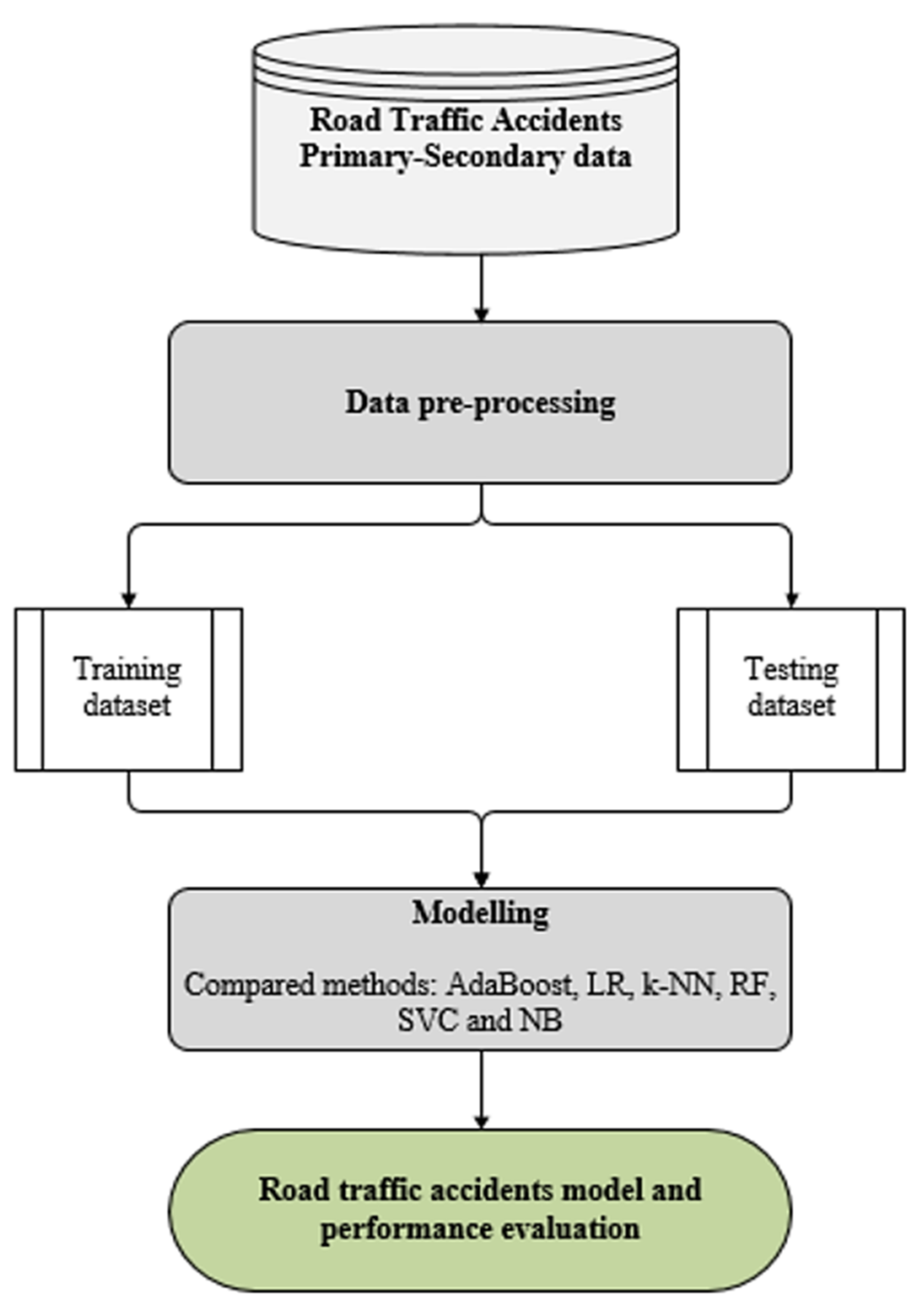
RTA Experimental Process
This section depicts the stages of the experimental process that were followed during the construction of the RTA model. The process consisted of five layers: type of dataset; data pre-processing, which involved data cleaning, dimensionality reduction, and preparation; data pre-processing was followed by sub-processes, namely, data training and testing; comparison analysis of the ML methods; and finally, the predicted RTA model evaluated. The process is illustrated in Figure 1 below.
3.4. Dataset and Statistical Analysis
Experiments were conducted using real-life data obtained from the Gauteng Department of Community Safety (GDCS). The collected dataset was compiled over a four-year duration. Ethical clearance was obtained from the ethics committee and the department to collect the historical dataset (Ref: 2020SCiiS04). The dataset included recordings of road traffic accidents over major highways in Gauteng province. Some features were omitted during data preparation because they contained insufficient entries. Then, features with 5% missing values were used during the analysis and handled using missing data strategies. Extensive data pre-processing was performed, resulting in a cleaned dataset containing 46,692 instances and 8 attributes, as shown in Table 1. The data had missing values that were handled using several missing value methods, as discussed in Section 3.2 above.
RTA Dataset
Table 1 contains a list of features and events employed for the study. The Events column shows that there are four classes. Due to the kind of dataset, the study was solving a multi-class problem. Multi-class classification refers to a classification task that contains more than two classes; it makes assumptions that each sample is assigned to only one label [53].
During data exploration, different numbers of parameters (features) were chosen to compute the classification model. This section of the paper statistically summarises the dataset to observe how data were distributed among the parameters/features. Figure 2a shows a distribution of road traffic accidents based on the Primary Cause. Stationary vehicles were the main contributors to causing primary accidents and were followed by crashes. This means that if the transport authorities or emergency authorities should prioritise clearing stationary vehicles on the roads, this may significantly reduce the high number of initial incidents. Figure 2b shows that five lanes were open when minor accidents occurred, followed by four lanes, which mean most incidents occur when most lanes are unavailable. The numbers in the figure are ordered according to the high number of vehicles or incidents. This figure reveals that accidents occur when fewer lanes are open on the freeway.
Figure 2c shows that when the roads were wet, fewer accidents were recorded. The wet road feature consists of No and Yes variables, with the No wet roads contributing significantly more to the road accident records when compared with the Yes variable. This means that from the obtained dataset, most of the accidents are not affected by wet roads. Figure 2d shows the data distribution for secondary accidents. The secondary accident’s cause is made up of seven variables, i.e., Crash, Stationary Vehicle, Road Construction, Load Lost, Routine Road Maintenance, Police and Military, and Fire. It is observed that Crash accidents contribute more to secondary accidents, which can be due to delayed clearance of the initial accidents. An overall observation is that if initial accidents are cleared on time, this could reduce the number of secondary accidents.
Figure 3 shows the distribution of the dependent (events) variables. It demonstrates that Minor events contribute more than None, Major and Natural Disaster events. This means that most of the contributing RTAs happen during Minor accidents. In addition, it means Minor accidents are those which contribute to the high number of road accidents, and they can result in lane closures, an increase in the number of stationary vehicles, and delayed clearance. In terms of the None event, the dataset containing this class was originally the resulting label or class. Furthermore, the data also contained unknown or unlabelled instances, which could be the result of capturing errors or the system being offline to capture real-time information with labels.
3.5. Model Evaluation
The study evaluated the performance of the classification model using accuracy, RMSE, precision, recall, and area under the ROC curve based on the confusion matrix. A low value for RMSE indicates that the predicted model can be considered, whereas a higher accuracy value indicates outstanding performance [55]. Formulas for calculating the evaluation metrics are shown in Equations (2)–(6):
The accuracy evaluation metrics in Equation (1) are calculated using the following: true positive (TP), true negative (TN), false negative (FN), and false positive (FP). The metrics correspond to the instances that are correctly classified [56].
Precision and recall represent the ratio of positive instances (TP) that are correct in the RTA dataset. High values of precision and recall indicate that the returned results are significant. The computation formulas are captured in Equations (3) and (4):
Model validation was carried out using the area under the ROC curve, as defined by Equation (5). The ROC curve can assist in determining the best threshold values produced by plotting sensitivity (TPR—true positive rate) against the specificity (FPR—false positive rate), indicating the proportion of RTAs. The study computed the AUC, the purpose of which is to deal with problems that contain a skewed data distribution to avoid over-fitting to a single class. An outstanding model will achieve an AUC near 1, which means good performance; a poor model will achieve an AUC near 0.5, which means poor performance [57]. The AUC can be defined using Equation (5), representing the average overall sensitivity values of FPR and TPR.
Equation (6) shows how the RMSE formulation, which determines the difference between the predicted and actual values, is computed as , with being the observed value for and being the model’s predicted value.
4. Dimensionality Reduction
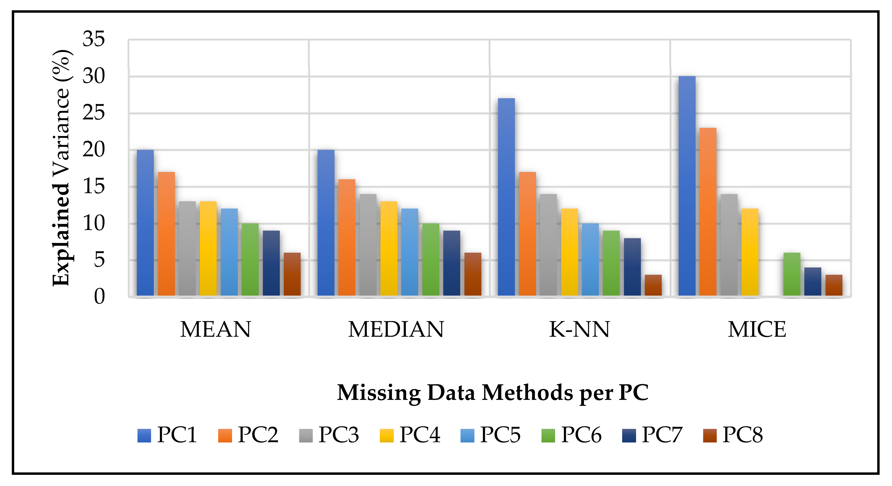
In this section of the study, dimensionality reduction techniques, PCA and LDA, were applied to the dataset. PCA was applied to the dataset to reduce its dimensionality by identifying the most important and best-contributing features. PCA can be used as an exploratory data analysis technique, with PC1 describing the highest variance in the RTA data. Four datasets were used to construct Figure 4: mean, median, k-NN, and MICE. Missing data methods were applied to the original data to handle the missingness. For the four augmented datasets, three principal components (PCs) and linear discriminants (LDs) were used during the experiments discussed in Section 5 and in designing the 3D graphs in Figure 5. LDA mainly considers the response/state variable chosen by the classifier. Linear discriminant analysis was used to reduce the different feature sets and predict RTA states by using different features in this paper. Overall, the PC results captured the following percentages for the datasets:
- (1)
- Mean missing data method: PC1—20%, PC2—17%, and PC3—13%, which explained 50% of the overall dataset;
- (2)
- Median method: PC1—20%, PC2—16%, and PC3—14%, which explained 50%;
- (3)
- k-NN method: PC1—27%, PC2—17%, and PC3—14%, which explained 58%;
- (4)
- MICE method: PC1—30%, PC2—23%, and PC3—14%, which explained 67% (of the overall dataset).
Figure 4.
The proportions of variance explained for the RTA dataset.

Figure 5.
Three-dimensional principle component plots using the four missing data methods: (a) mean, (b) median, (c) k-NN, and (d) MICE.
Figure 5.
Three-dimensional principle component plots using the four missing data methods: (a) mean, (b) median, (c) k-NN, and (d) MICE.

The MICE dataset explained more of the PCs when compared with the other PCs. In this study, the main idea behind PCA was to identify the correlation between the RTA features.
Figure 5 shows the 3D scatter plots for PC1, PC2, and PC3 components against four events to better understand the data distribution. The distributions of PC1, PC2, and PC3 are represented by the colours yellow, blue and viridis, respectively. Figure 5 presents the data variance distribution for the RTA dataset.
Figure 5a shows that PC2 was distributed more than PC1 and PC3. On the other hand, some outliers were observed from PC3. Outliers can affect the final results of the analysis of the study.
Figure 5b shows that PC1 and PC2 contributed most of the variance in the data distribution, when compared with PC3. Some outliers are observed from PC2, which were moving towards PC3 using the median RTA dataset.
Figure 5c shows that PC1 and PC3 were moving more towards PC3, which appeared to be overlapping with PC2. It can also be observed that PC1 was moving away from PC2 and PC3, with some outliers from PC1. The figure shows some correlation between PC2 and PC3.
In Figure 5d, it can be observed that PC2 contributed more to the data points when compared with the other PCs. PC1 shows fewer data points moving towards PC3.
5. Results and Discussion
This section discusses and presents the results of the six classifiers, namely, NB, LR, k-NN, AdaBoost, RF, and SVM. The classification comparisons are discussed in detail to observe which methods/algorithms best predict RTAs.
5.1. Comparison Results
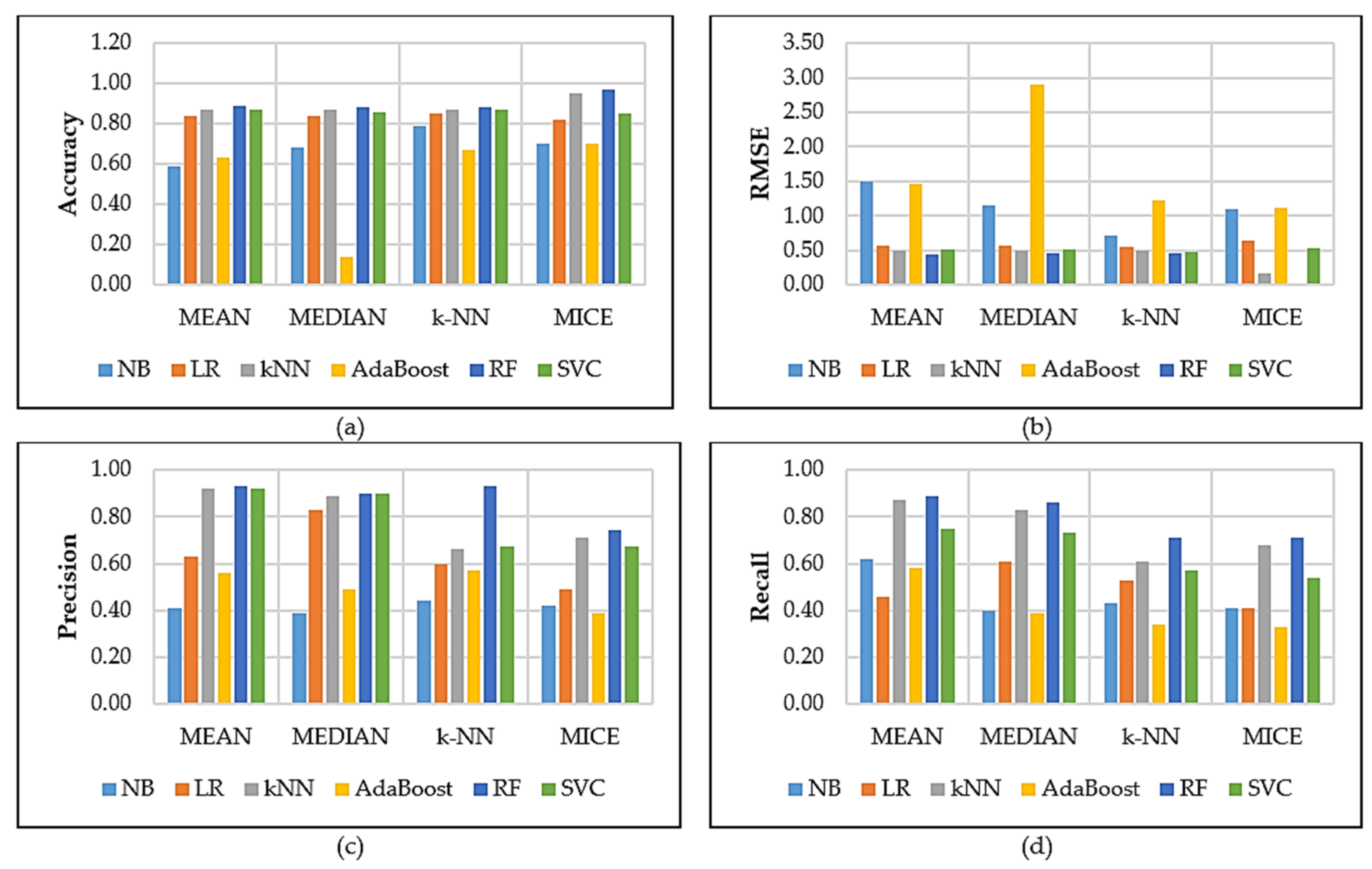
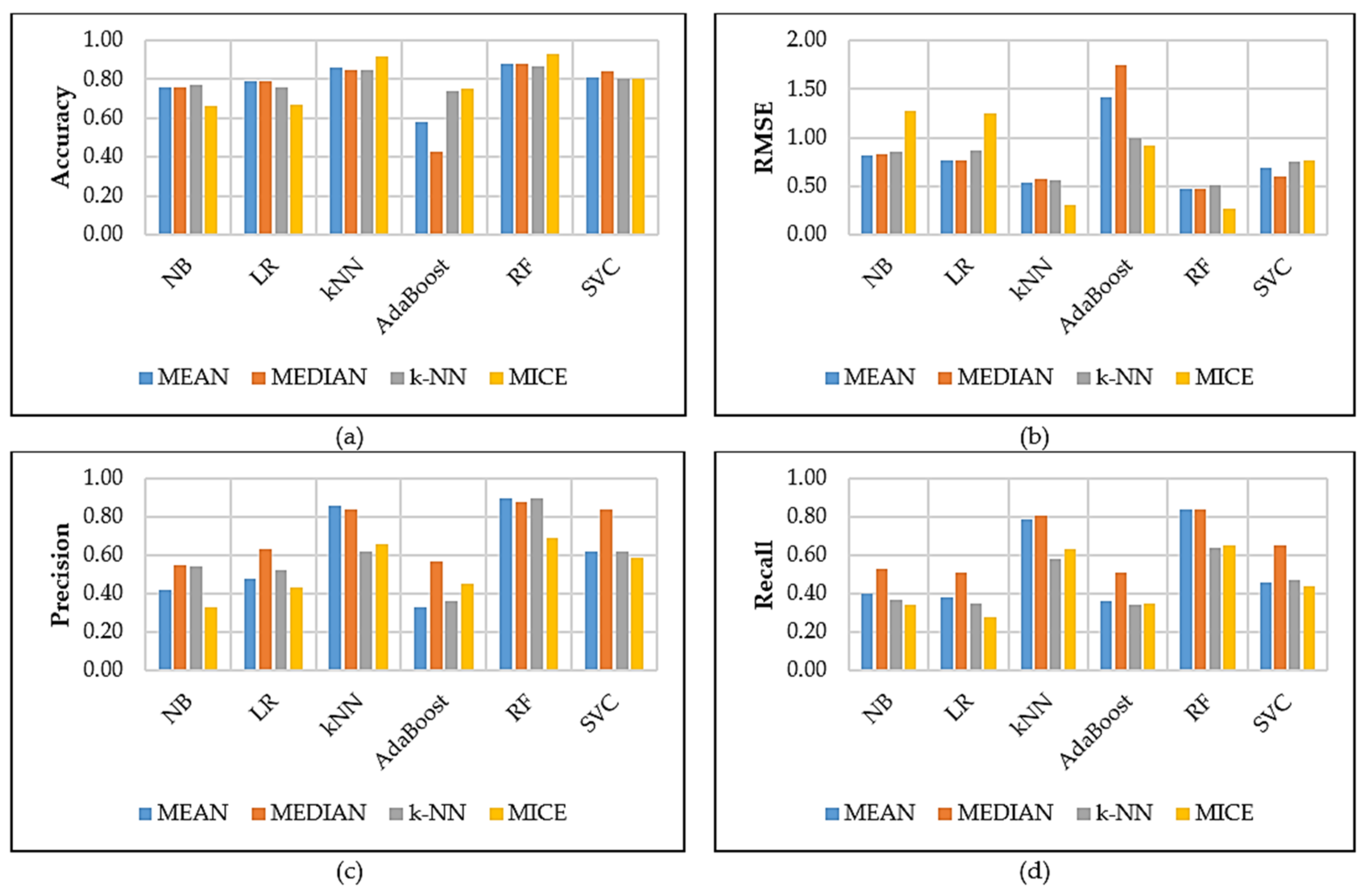
Figure 6 and Figure 7 show the results for the default and optimised model settings. The results report the performance of the observed classifiers based on different missing data methods. The following can be observed: the results obtained using default Figure 6a settings for the six classifiers did not perform well across the different missing data methods applied to the RTA dataset. However, RF (97%) performed much better in terms of all the model evaluations. These results could be due to RF offering efficient test error estimates without experiencing any cost and offering reliable feature importance approximation. The AdaBoost classifier showed the lowest performance across all evaluation methods. AdaBoost could have performed poorly because it cannot handle data with outliers well. Figure 6b shows results obtained for RMSE where the RF model obtained the lowest value of 0.01, which means the model had lower errors when compared to the other methods. In terms of precision, the RF model achieved the best value of 93% when the mean and kNN missing value methods data was used in Figure 6c. Then results presented in Figure 6d for recall show that RF model obtained a high value of 89% when the mean missing value data method was utilised. In addition, MICE performed well across the used classifiers compared with the mean, k-NN, and median missing value methods.
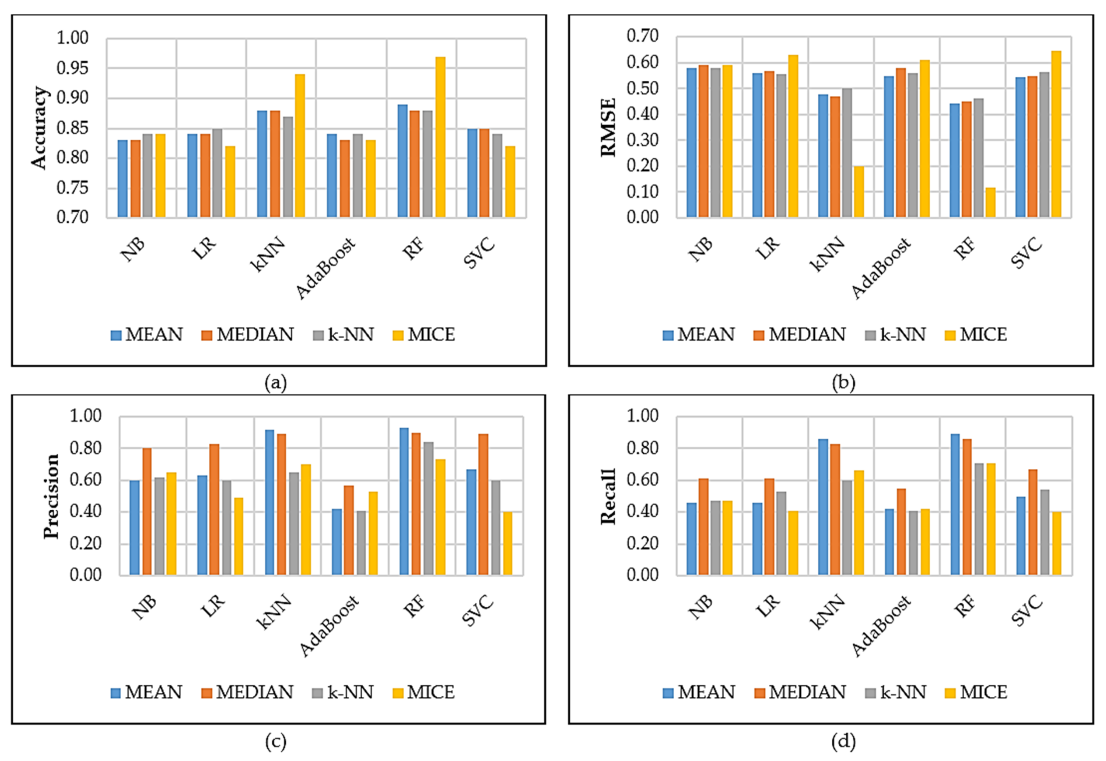
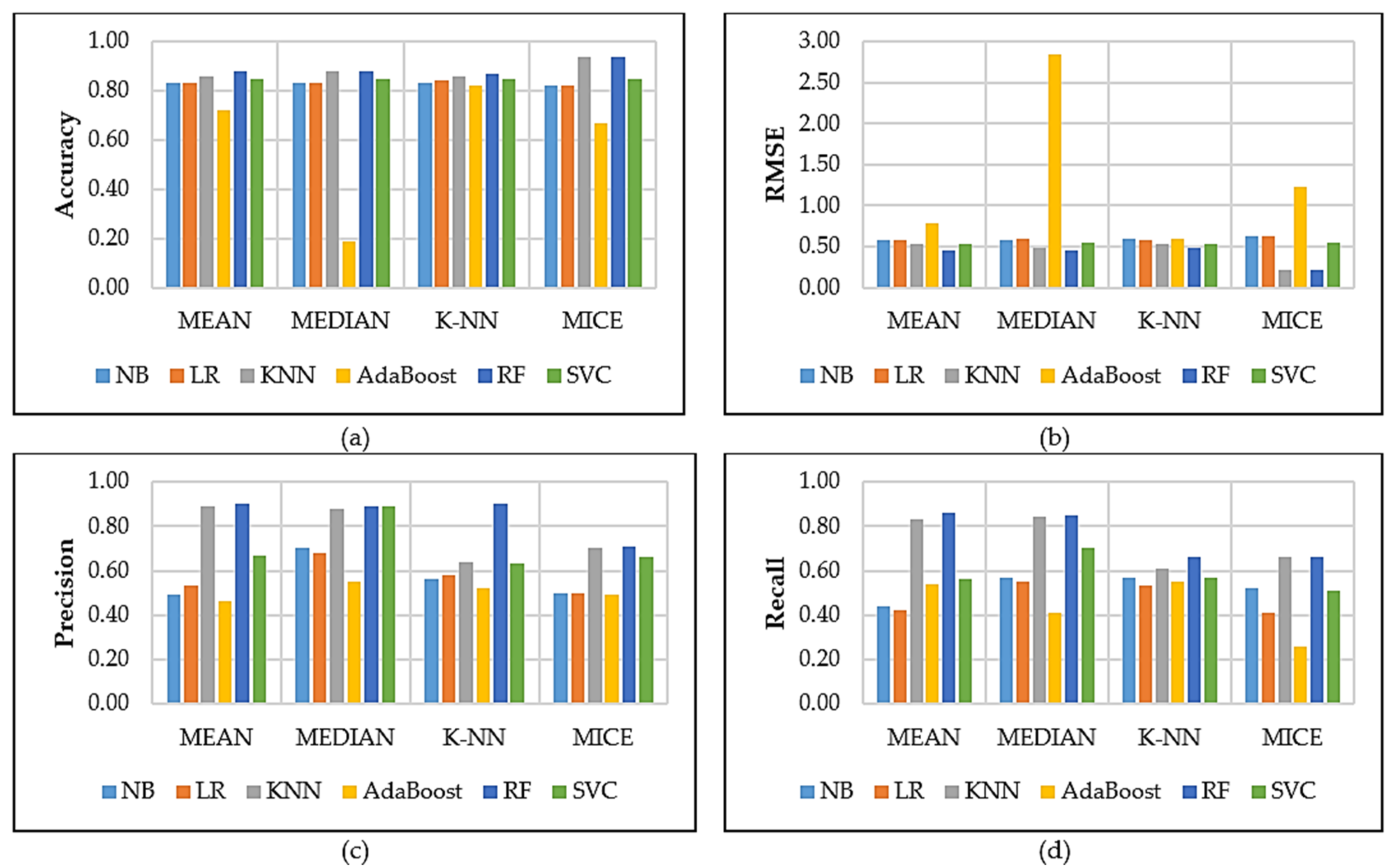
Concerning the Figure 7 model optimisation results, the following can be observed: Figure 7a RF performed slightly better overall than the other classifiers across all the evaluation methods with an accuracy of 97%. One possible reason is that RF can handle thousands of inputs without deleting any variables. The RF settings were tuned to entropy and n_estimators = 10. The RF results show that parameter tuning did not improve the results, as shown in Figure 7a. Furthermore, LR and SVC performed poorly when compared with the other classifiers. In terms of RMSE in Figure 7b, RF model obtained 0.12, which mean the model has low errors compared to the others. Figure 7c shows precision results, which revealed that the RF performed well by obtaining 93% when mean missing value data was considered. Finally, Figure 7d shows that RF achieved the best value of 89% compared with the other methods such as SVC, NB, kNN, LR and AdaBoost. In general, RF obtained promising results when compared with the other classifiers. The following graphs present results for PCA and LDA.
Figure 8 and Figure 9 contain graphical results computed using the RTA dataset. They include PCA and LDA dimensionality reduction techniques, which means reducing a large number of features to a smaller number of PCs. The results report the performance of the six classifiers based on four different missing data methods. The following is observed from the results: in the PCA results in Figure 8a, the RF classifier performed reliably and much better with accuracy (93%), precision and recall performance metrics when using MICE data. The MICE imputation method performed better compared with the other missing value methods because, as pointed out in Section 4, it captured 67% of the overall dataset. With a high RMSE, the AdaBoost classifier is the most poorly performing classifier. Figure 8b shows the results of the RMSE for all the augmented datasets and the results revealed that RF obtained a very low RMSE value of 0.27 compared to the other methods. Figure 8c show that the RF models achieved the best results in terms of precision, with MICE imputation methods achieving 93%. Then in Figure 8d, the graph presents recall results, which revealed that RF in terms of mean and median obtained 84%.
The LDA results in Figure 9a indicate that the RF (94%) and k-NN (94%) classifiers performed comparatively better than the other classifiers and the PCA results. AdaBoost (82%) was the classifier with the lowest performance results across all the evaluation metrics. In Figure 9b, the results show that kNN and RF methods best performed by achieving 0.22; in terms of the RMSE metric, the lowest values were obtained by RF and kNN when MICE imputation data is utilised. Figure 9c presents precision results with RF obtaining the best performance across all missing value methods compared to the others. Lastly, the Recall results graph in Figure 9d shows that RF, in terms of the mean missing value method, achieved the best value of 86%. The results mean that the LDA reduction method dataset obtained much better results when compared with the PCA technique. Furthermore, LDA performed best in multi-class classification problems. The LDA technique, when compared with the PCA, considers dependent variables during the creation of the LDs.
The results in Figure 8 and Figure 9 show that the application of PCA and LDA positively changed the performance of the classifiers. The RF model remained the best performing in terms of the overall results. This is in addition to the fact that Figure 6 and Figure 7 present a lower RMSE when compared with the Figure 8 and 9 results.
5.2. ROC Curve (AUC)
The area under the ROC curve is the ratio between 0.5 and 1, where values close to 0.5 indicate poor results, whereas values of 1 mean the best performance. The AUC is mainly implemented to evaluate and validate how robust the ML model is. In this study, the AUC for the MICE data performed better throughout the investigation compared with other missing data methods. The RF model, as seen in Figure 10, showed a performance of 99%; better than the other classifiers. Additionally, as shown in Figure 10, the AUC gives certainties of excellent classifications of the RF model.
6. Conclusions
This study investigated the strength of widely used ML classifiers for road traffic accident problems. The classifiers were NB, k-NN, AdaBoost, SVM, LR, and NB. These were evaluated with four missing data methods: MICE, k-NN, mean and median, and two-dimensionality reduction methods: PCA and LDA. Accuracy, RMSE, precision, recall, and the ROC curve (AUC) were the five performance metrics used to evaluate the ML models. The overall results revealed that RF performed marginally better across the experiments in terms of accuracy, precision, recall, and ROC (AUC) when compared with the other classifiers. RF had the lowest RMSE compared with all the other classifiers, indicating a better fit for the RF model. Overall findings of the study on this particular RTA dataset are as follows:
- (1)
- Statistical analysis included two-dimensionality reduction methods, with LDA obtaining promising results compared with PCA. In terms of missing data methods, MICE achieved good results;
- (2)
- A wide range of ML methods was applied due to their popularity and characteristics. It was observed from the empirical analysis that RF performed best when compared with the rest;
- (3)
- Furthermore, the AUC evaluation method was introduced to validate the classification results once the evaluation performance was assessed using accuracy, precision, and recall.
Some apparent limitations of the study are as follows: only a dataset from Gauteng province was utilised during the comparative analysis. The dataset contained a certain number of features for the specific area of interest, excluding other features that could have been beneficial to improving the model’s performance. The data only contained four events/targets for possible scenarios to incorporate subclasses into the data.
For future work, further hyperparameter tuning could improve the SVC model results because the classifier is more strongly influenced by proper parameter tuning. Future research could test other ML classifiers such as artificial neural networks and deep learning, testing similar methods with different datasets or provincial metro and expanding the data in years. The approach itself is a contribution that benefits RTA stakeholders such as model developers and researchers, and inform policymakers and transportation safety designers in terms of actions relating to modern traffic safety control and actual predictive models, which will help develop the field of transportation.
Author Contributions
T.B.: conceptualisation, data curation, formal analysis, methodology, experiments, writing—review and editing, and result validation. W.D. and B.S.P. project administration, supervision, conceptualisation, and critical revision. All authors have read and agreed to the published version of the manuscript.
Funding
This research did not receive external funding.
Institutional Review Board Statement
Not applicable.
Informed Consent Statement
Informed consent was obtained from all subjects involved in the study.
Data Availability Statement
The data are not publicly available due to restrictions from the subject’s agreement.
Acknowledgments
The Department of Applied Information Systems, the Institute for Intelligent Systems, and the University of Johannesburg supported this research. The authors would also like to thank the Gauteng Department of Community Safety, South Africa, for permitting the use of the RTA dataset.
Conflicts of Interest
The authors do not have any conflict of interest with other entities or researchers.
References
- World Economic Forum. The Number of Cars Worldwide Is Set to Double by 2040. 2016. Available online: https://www.weforum.org/agenda/2016/04/the-number-of-cars-worldwide-is-set-to-double-by-2040 (accessed on 8 February 2021).
- World Health Organisation. Global Status Report on Road Safety. 2015. Available online: https://www.who.int/violence_injury_prevention/road_safety_status/2015/en/ (accessed on 25 January 2021).
- World Health Organisation. Global Status Report on Road Safety. 2018. Available online: https://www.who.int/violence_injury_prevention/road_safety_status/2018/en/ (accessed on 25 January 2021).
- National Institute of Statistics and Economic Studies (INSEE). Road Accidents. 2020. Available online: https://www.insee.fr/en/metadonnees/definition/c1116 (accessed on 25 January 2021).
- Wesson, H.K.; Boikhutso, N.; Hyder, A.A.; Bertram, M.; Hofman, K.J. Informing road traffic intervention choices in South Africa: The role of economic evaluations. Global Health Action. 2016, 9, 30728. [Google Scholar] [CrossRef] [PubMed] [Green Version]
- Wang, J.; Liu, B.; Fu, T.; Liu, S.; Stipancic, J. Modelling when and where a secondary accident occurs. Accid. Anal. Prev. 2019, 130, 160–166. [Google Scholar] [CrossRef]
- World Health Organisation. Global Status Report on Road Safety. 2019. Available online: https://www.who.int/violence_injury_prevention/road_safety_status/2019/en/ (accessed on 8 January 2021).
- Makaba, T.; Gatsheni, B. A decade bibliometric review of road traffic accidents and incidents: A computational perspective. In Proceedings of the 2019 International Conference on Computational Science and Computational Intelligence (CSCI), Las Vegas, NV, USA, 5–7 December 2019; IEEE: New York, NY, USA, 2019; pp. 510–516. [Google Scholar]
- Sánchez González, S.; Bedoya-Maya, F.; Calatayud, A. Understanding the Effect of Traffic Congestion on Accidents Using Big Data. Sustainability 2021, 13, 7500. [Google Scholar] [CrossRef]
- Zhang, H.; Khattak, A. What is the role of multiple secondary incidents in traffic operations? J. Transp. Eng. 2010, 136, 986–997. [Google Scholar] [CrossRef] [Green Version]
- Zhan, C.; Shen, L.; Hadi, M.A.; Gan, A. Understanding the Characteristics of Secondary Crashes on Freeways; No. 08-1835; Transportation Research Board: Washington, DC, USA, 2008. [Google Scholar]
- Ramageri, B.M. Data mining techniques and applications. Indian J. Comput. Sci. Eng. 2010, 1, 301–305. [Google Scholar]
- Li, L.; Shrestha, S.; Hu, G. Analysis of road traffic fatal accidents using data mining techniques. In Proceedings of the 2017 IEEE 15th International Conference on Software Engineering Research, Management and Applications (SERA), London, UK, 7–9 June 2017; IEEE: New York, NY, USA, 2017; pp. 363–370. [Google Scholar]
- Alpaydin, E. Introduction to Machine Learning; MIT Press: Cambridge, MA, USA, 2020. [Google Scholar]
- Mohri, M.; Rostamizadeh, A.; Talwalkar, A. Foundations of Machine Learning; MIT Press: Cambridge, MA, USA, 2018. [Google Scholar]
- Expert AI. What Is Machine Learning? A Definition. 2020. Available online: https://www.expert.ai/blog/machine-learning-definition/ (accessed on 20 March 2021).
- Costanza, R.; Daly, L.; Fioramonti, L.; Giovannini, E.; Kubiszewski, I.; Mortensen, L.F.; Pickett, K.E.; Ragnarsdottir, K.V.; De Vogli, R.; Wilkinson, R. Modelling and measuring sustainable wellbeing in connection with the UN Sustainable Development Goals. Ecol. Econ. 2016, 130, 350–355. [Google Scholar] [CrossRef]
- Sachs, J.D.; Kroll, C.; Lafortune, G.; Fuller, G.; Woelm, F. Sustainable Development Report: The Decade of Action for the Sustainable Development Goals. 2021. Available online: https://s3.amazonaws.com/sustainabledevelopment.report/2021/2021-sustainable-development-report.pdf (accessed on 21 March 2021).
- Asiri, S. Machine Learning Classification, towards Data Science. 2018. Available online: https://towardsdatascience.com/machine-learning-classifiers-a5cc4e1b0623 (accessed on 20 December 2020).
- Waseem, M. How to Implement Classification in Machine Learning, Data Science with Python. 2021. Available online: https://www.edureka.co/blog/classification-in-machine-learning/#classification (accessed on 5 April 2021).
- Sarangam, A. Classification in Machine Learning: A Comprehensive Guide, Jigsaw. 2021. Available online: https://www.jigsawacademy.com/blogs/ai-ml/classification-in-machine-learning (accessed on 8 August 2021).
- Priyanka, A.; Sathiyakumari, K. A comparative study of classification algorithm using accident data. Int. J. Comput. Sci. Eng. Technol. 2014, 5, 1018–1023. [Google Scholar]
- AlMamlook, R.E.; Kwayu, K.M.; Alkasisbeh, M.R.; Frefer, A.A. Comparison of machine learning algorithms for predicting traffic accident severity. In Proceedings of the 2019 IEEE Jordan International Joint Conference on Electrical Engineering and Information Technology (JEEIT), Amman, Jordan, 9–11 April 2019; IEEE: New York, NY, USA, 2019; pp. 272–276. [Google Scholar]
- Labib, M.F.; Rifat, A.S.; Hossain, M.M.; Das, A.K.; Nawrine, F. Road accident analysis and prediction of accident severity by using machine learning in Bangladesh. In Proceedings of the 2019 7th International Conference on Smart Computing & Communications (ICSCC), Miri, Malaysia, 28–30 June 2019; IEEE: New York, NY, USA, 2019; pp. 1–5. [Google Scholar]
- Lee, J.; Yoon, T.; Kwon, S.; Lee, J. Model evaluation for forecasting traffic accident severity in rainy seasons using machine learning algorithms: Seoul City study. Appl. Sci. 2020, 10, 129. [Google Scholar] [CrossRef] [Green Version]
- Ijaz, M.; Zahid, M.; Jamal, A. A comparative study of machine learning classifiers for injury severity prediction of crashes involving three-wheeled motorised rickshaw. Accid. Anal. Prev. 2021, 154, 106094. [Google Scholar] [CrossRef] [PubMed]
- Sangare, M.; Gupta, S.; Bouzefrane, S.; Banerjee, S.; Muhlethaler, P. Exploring the forecasting approach for road accidents: Analytical measures with hybrid machine learning. Expert Syst. Appl. 2021, 167, 113855. [Google Scholar] [CrossRef]
- Zong, F.; Xu, H.; Zhang, H. Prediction for traffic accident severity: Comparing the Bayesian network and regression models. Math. Probl. Eng. 2013, 2013, 475194. [Google Scholar] [CrossRef] [Green Version]
- Park, H.; Haghani, A. Real-time prediction of secondary incident occurrences using vehicle probe data. Transportation Research Part C Emerg. Technol. 2016, 70, 69–85. [Google Scholar] [CrossRef]
- Bahiru, T.K.; Singh, D.K.; Tessfaw, E.A. Comparative study on data mining classification algorithms for predicting road traffic accident severity. In Proceedings of the 2018 Second International Conference on Inventive Communication and Computational Technologies (ICICCT), Coimbatore, India, 20–21 April 2018; IEEE: New York, NY, USA, 2018; pp. 1655–1660. [Google Scholar]
- Kumeda, B.; Zhang, F.; Zhou, F.; Hussain, S.; Almasri, A.; Assefa, M. Classification of road traffic accident data using machine learning algorithms. In Proceedings of the 2019 IEEE 11th International Conference on Communication Software and Networks (ICCSN), Chongqing, China, 12–15 June 2019; IEEE: New York, NY, USA, 2019; pp. 682–687. [Google Scholar]
- Jha, A.N.; Chatterjee, N.; Tiwari, G. A performance analysis of prediction techniques for impacting vehicles in hit-and-run road accidents. Accid. Anal. Prev. 2021, 157, 106164. [Google Scholar] [CrossRef] [PubMed]
- Valenti, G.; Lelli, M.; Cucina, D. A comparative study of models for the incident duration prediction. Eur. Transp. Res. Rev. 2010, 2, 103–111. [Google Scholar] [CrossRef] [Green Version]
- Vlahogianni, E.I.; Karlaftis, M.G.; Orfanou, F.P. Modelling the effects of weather and traffic on the risk of secondary incidents. J. Intell. Transp. Syst. 2012, 16, 109–117. [Google Scholar] [CrossRef]
- Dogru, N.; Subasi, A. Traffic accident detection using random forest classifier. In Proceedings of the 2018 15th learning and technology conference (L&T), Jeddah, Saudi Arabia, 26–28 February 2018; IEEE: New York, NY, USA, 2018; pp. 40–45. [Google Scholar]
- Makaba, T.; Doorsamy, W.; Paul, B.S. Exploratory framework for analysing road traffic accident data with validation on Gauteng province data. Cogent Eng. 2020, 7, 1834659. [Google Scholar] [CrossRef]
- Zambrano-Martinez, J.L.; Calafate, C.T.; Soler, D.; Cano, J.C.; Manzoni, P. Modeling and characterisation of traffic flows in urban environments. Sensors 2018, 18, 2020. [Google Scholar] [CrossRef] [Green Version]
- Makaba, T.; Doorsamy, W.; Paul, B.S. Bayesian Network-Based Framework for Cost-Implication Assessment of Road Traffic Collisions. Int. J. Intell. Transp. Syst. Res. 2021, 19, 240–253. [Google Scholar] [CrossRef]
- Mir, Z.H.; Filali, F. An adaptive Kalman filter based traffic prediction algorithm for urban road network. In Proceedings of the 2016 12th International Conference on Innovations in Information Technology, Al-Ain, United Arab Emirates, 28–30 November 2016; IEEE: New York, NY, USA, 2016; pp. 1–6. [Google Scholar]
- Budiawan, W.; Saptadi, S.; Tjioe, C.; Phommachak, T. Traffic accident severity prediction using Naive Bayes algorithm—A case study of Semarang Toll Road. IOP Conf. Ser. Mater. Sci. Eng. 2019, 598, 012089. [Google Scholar] [CrossRef]
- Kim, D.; Jung, S.; Yoon, S. Risk Prediction for Winter Road Accidents on Expressways. Appl. Sci. 2021, 11, 9534. [Google Scholar] [CrossRef]
- Li, P.; Abdel-Aty, M.; Yuan, J. Real-time crash risk prediction on arterials based on LSTM-CNN. Accid. Anal. Prev. 2020, 135, 105371. [Google Scholar] [CrossRef] [PubMed]
- Twala, B. Dancing with dirty road traffic accidents data: The case of Gauteng Province in South Africa. J. Transp. Saf. Secur. 2012, 4, 323–335. [Google Scholar] [CrossRef]
- Yu, H.; Ji, N.; Ren, Y.; Yang, C. A special event-based K-nearest neighbor model for short-term traffic state prediction. IEEE Access. 2019, 7, 81717–81729. [Google Scholar] [CrossRef]
- Zhang, X.; Waller, S.T.; Jiang, P. An ensemble machine learning-based modelling framework for analysis of traffic crash frequency. Comput. -Aided Civ. Infrastruct. Eng. 2020, 35, 258–276. [Google Scholar] [CrossRef]
- Chen, M.M.; Chen, M.C. Modelling road accident severity with Comparisons of Logistic Regression, Decision Tree and Random Forest. Information 2020, 11, 270. [Google Scholar] [CrossRef]
- Lin, Y.; Li, R. Real-time traffic accidents post-impact prediction: Based on crowdsourcing data. Accid. Anal. Prev. 2020, 145, 105696. [Google Scholar] [CrossRef] [PubMed]
- Parsa, A.B.; Taghipour, H.; Derrible, S.; Mohammadian, A.K. Real-time accident detection: Coping with imbalanced data. Accid. Anal. Prev. 2019, 129, 202–210. [Google Scholar] [CrossRef]
- Tang, J.; Liang, J.; Han, C.; Li, Z.; Huang, H. Crash injury severity analysis using a two-layer stacking framework. Accid. Anal. Prev. 2019, 122, 226–238. [Google Scholar] [CrossRef] [PubMed]
- Makaba, T.; Dogo, E. A comparison of strategies for missing values in data on machine learning classification algorithms. In Proceedings of the 2019 International Multidisciplinary Information Technology and Engineering Conference (IMITEC), Vanderbijyl Park, South Africa, 21–22 November 2019; IEEE: New York, NY, USA, 2019; pp. 1–7. [Google Scholar]
- Liu, Y.; Brown, S.D. Comparison of five iterative imputation methods for multivariate classification. Chemom. Intell. Lab. Syst. 2013, 120, 106–115. [Google Scholar] [CrossRef]
- Chowdhury, K.R. KNN Imputer: A Robust Way to Impute Missing Values Using Scikit-Learn. 2020. Available online: https://www.analyticsvidhya.com/blog/2020/07/knnimputer-a-robust-way-to-impute-missing-values-using-scikit-learn/ (accessed on 22 December 2020).
- Mokoatle, M.; Marivate, V.; Bukohwo, M.E. Predicting road traffic accident severity using accident report data in South Africa. In Proceedings of the 20th Annual International Conference on Digital Government Research, Dubai, United Arab Emirates, 18–20 June 2019; ACM: New York, NY, USA, 2019; pp. 11–17. [Google Scholar]
- Buuren, S.V.; Groothuis-Oudshoorn, K. Mice: Multivariate imputation by chained equations in R. J. Stat. Softw. 2010, 45, 1–68. [Google Scholar]
- Ramani, R.G.; Shanthi, S. Classifier prediction evaluation in modelling road traffic accident data. In Proceedings of the 2012 IEEE International Conference on Computational Intelligence and Computing Research, Coimbatore, India, 18–20 December 2012; IEEE: New York, NY, USA, 2012; pp. 1–4. [Google Scholar]
- Gutierrez-Osorio, C.; Pedraza, C. Modern data sources and techniques for analysis and forecast of road accidents: A review. J. Traffic Transp. Eng. 2020, 7, 432–446. [Google Scholar] [CrossRef]
- Cigdem, A.; Ozden, C. Predicting the severity of motor vehicle accident injuries in Adana-turkey using machine learning methods and detailed meteorological data. Int. J. Intell. Syst. Appl. Eng. 2018, 6, 72–79. [Google Scholar]
Figure 1.
RTAs experimental procedure.

Figure 2.
RTA data distribution over different features: (a) primary cause; (b) no. of travel lanes; (c) wet road; and (d) secondary cause.
Figure 2.
RTA data distribution over different features: (a) primary cause; (b) no. of travel lanes; (c) wet road; and (d) secondary cause.

Figure 3.
RTA events data distribution.

Figure 6.
Default settings performance results.

Figure 7.
Model optimisation performance results.

Figure 8.
PCA performance results.

Figure 9.
LDA performance results.

Figure 10.
Comparison of the AUC results.


Table 1.
RTA features and events.
| No. | Features | Data Type | Events |
|---|---|---|---|
| 1. | Primary Cause | Categorical | Major |
| 2. | Primary Sub Cause | Categorical | Minor |
| 3. | Secondary Cause | Categorical | Natural disaster |
| 4. | Wet Road | Categorical | None |
| 5. | No. of Travel Lanes | Numeric | Unknown |
| 6. | No. of Vehicles Involved | Numeric | - |
| 7. | Roadway Name | Categorical | - |
| 8. | Date Time | Date time | - |
Publisher’s Note: MDPI stays neutral with regard to jurisdictional claims in published maps and institutional affiliations. |
© 2022 by the authors. Licensee MDPI, Basel, Switzerland. This article is an open access article distributed under the terms and conditions of the Creative Commons Attribution (CC BY) license (https://creativecommons.org/licenses/by/4.0/).
Share and Cite
MDPI and ACS Style
Bokaba, T.; Doorsamy, W.; Paul, B.S. Comparative Study of Machine Learning Classifiers for Modelling Road Traffic Accidents. Appl. Sci. 2022, 12, 828. https://0-doi-org.brum.beds.ac.uk/10.3390/app12020828
AMA Style
Bokaba T, Doorsamy W, Paul BS. Comparative Study of Machine Learning Classifiers for Modelling Road Traffic Accidents. Applied Sciences. 2022; 12(2):828. https://0-doi-org.brum.beds.ac.uk/10.3390/app12020828
Chicago/Turabian StyleBokaba, Tebogo, Wesley Doorsamy, and Babu Sena Paul. 2022. "Comparative Study of Machine Learning Classifiers for Modelling Road Traffic Accidents" Applied Sciences 12, no. 2: 828. https://0-doi-org.brum.beds.ac.uk/10.3390/app12020828
Note that from the first issue of 2016, this journal uses article numbers instead of page numbers. See further details here.