Intelligent Trajectory Prediction Algorithm for Reentry Glide Target Based on Intention Inference

Featured Application

The method proposed can be used of accurate trajecotory prediction of reentry glide target based on intention inference. And it also provides ideas for intention inference of target using deep neural network.

Abstract

Aimed at the problem of the insufficient utilization of intention information and flight data for the trajectory prediction of a reentry glide target, an intelligent trajectory prediction algorithm based on intention inference was proposed. Firstly, a control parameter prediction network was developed to predict the variation of the control parameter values. Secondly, based on the Gaussian mixture model and Dubins circle, the importance of strategic places was modeled, the functional relationship between the strategic places and trajectories was established, and the influence factors of target threat were analyzed. Subsequently, an intention inference network was designed, which can accurately identify the key point the target intends to attack and realize the nonlinear calculation of the target’s threat value. Finally, according to the common guidance law of reentry glide target, the lateral sign-variation rule was designed to carry out the target trajectory prediction based on intention inference. Simulation revealed that the parameter prediction network designed in this paper can realize the modification of filtering control parameters and effectively predict the value of these parameters. Moreover, taking the result of intention inference network, trajectory prediction in different prediction cases was accomplished. The maximal error of spatial distance (MESD) of the proposed method was less than 9 km when the prediction time was 100 s, and the best result was obtained in the long-term prediction. Compared with other mainstream prediction methods, the proposed method obtained the best prediction accuracy.

1. Introduction

Reentry glide targets can glide in near space with high speed and mobility. This type of target usually has a flight speed higher than Mach 5, a longitudinal maneuverable range of tens of kilometers, and a lateral maneuverable range of hundreds of kilometers [1]. Compared with a ballistic target, its longitudinal and lateral maneuverability make it more difficult to precisely predict its trajectory. Therefore, the reentry glide target has been a great challenge for interceptors that realize handover between midcourse and terminal guidance according to high-probability region prediction [2].

At present, there are several excellent control algorithms [3,4] for hypersonic vehicles, while research on its trajectory prediction is still in its infancy. According to the prediction mechanism, the current trajectory prediction methods for reentry glide targets can be divided into three types: prediction through control parameter estimation; prediction by maneuver mode identification; and prediction using intention inference.

The first type of method entails obtaining the prediction trajectory by selecting the suitable control parameters and iterative integration. Based on the aerodynamic model of the reentry glide target, Zhai D.L. et al. [5] proposed a group of control parameters with a simple variation law through simulation analysis, which has a good prediction effect for the HTV-2 target. Li S.J. et al. [6] introduced a new control parameter for the problem that the variation law of control parameters is not easy to predict in the literature [5]. The simulation showed that the variation law of this new control parameter was easier to estimate. Han C.Y. et al. [7] simplified the aerodynamic force on a reentry glide target and obtained the simplified dynamic model. On this basis, the dynamic equation was deduced, and the trajectory prediction method was proposed. The above methods can effectively analyze the model, estimate the variation of control parameters, and predict the trajectory; however, the correlation between the prediction method and the flight data are not strong, as the prediction accuracy is limited by fitting the variation law of the control parameter with a simple function. Experiments in this paper have shown that it can lead to hundreds of kilometers of errors in long-term predictions.

The second type of method to predict trajectories involves identifying the maneuvering mode of the target. Ferreira et al. [8] and Chen et al. [9] analyzed the long-period motion of equilibrium glide, fitted skip glide into the oscillation curve by Liouville transformation and the multi-scale theory method, and provided the formula of skip times. Vinh et al. [10,11] analyzed the second-order approximate solutions of skip glide and equilibrium glide of targets with the constant attack angle, but the solutions were fairly complex. Lu et al. [12] regarded the quasi-equilibrium glide state of lift vehicles as a regular perturbation problem, decomposed the longitudinal trajectory of quasi-equilibrium glide into the combination of equilibrium glide and high-order terms, and analyzed the error between the real solution and the low-order solution. Cheng Y.P. et al. [13] accomplished trajectory prediction by analyzing the maneuvering mode of the target, generating a corresponding training set, training a support vector machine classifier, and combining it with an extended Kalman filter algorithm. However, the above methods only have good effects on trajectory prediction in partial maneuvering modes, while using training sets or networks to predict trajectories lacks a modeling basis, which may reduce the prediction accuracy and lead to the rapid divergence of prediction errors

The above two types of trajectory prediction methods mainly analyze the observation information of the target to realize prediction, which is insufficient in the modern situation analysis of strategic places and guidance mechanism of the target and may accelerate the accumulation of long-time trajectory prediction errors. Therefore, introducing auxiliary information for trajectory prediction is a useful method to improve prediction accuracy. As auxiliary information, the attack intention of the target plays an important role in improving prediction accuracy and has been widely used in aircraft trajectory prediction. Yu L. et al. [14] proposed a trajectory predictor based on the interacting multiple model (IMM) algorithm guided by the spatial and temporal information in the intent. Inspired by search strategies used in artificial intelligence, Guillermo et al. proposed a novel approach in which a search tree is generated to evaluate possible intent maneuvers at each point [15]. Further analyses of target attack intentions to realize the trajectory prediction of reentry glide targets have a good application value. Zhang K. et al. [16] discussed the key technology of reentry glide target trajectory prediction from the four aspects of establishing a prediction model, correcting the prediction error, identifying the guidance law, and inferring the target intention, and proposed a trajectory prediction theory combining state information and attack intention. Accordingly, based on the assumption that target intention is our strategic places, the maneuvering mode of the target is deduced based on Bayesian theory, and trajectory prediction is realized based on Monte Carlo sampling [17]. Hu Y.D. et al. [18] used an autoregressive model to identify maneuver modes, combined target intention with Bayesian theory to obtain the target’s state iteration dynamic equation, and selected prediction methods based on the effects. Combined with relevant intention information, the above methods further simplify the prediction model and effectively realize trajectory prediction. However, the uncertainty of the Bayesian process and sampling method may produce errors.

With the development of deep learning technology, fitting complex functions using a deep network has a favorable effect. In particular, recurrent neural networks (RNN) and long- and short-term memory networks (LSTM) [19] have beneficial effects on sequential feature extraction and sequential rule learning [20]. Trajectory prediction methods based on deep neural networks have also been widely applied in the field of aircraft trajectory prediction [21,22]. Recently, the temporal network has also been used in the trajectory prediction of reentry glide targets. Cai Y.L. et al. [23] designed a trajectory classifier and predictor based on the LSTM network and realized the trajectory prediction of non-ballistic targets driven by pure data. Xie Y. et al. [24] designed a gated recurrent unit (GRU) network based on a double-channel network that generates a prediction data set and carried out the trajectory prediction of high-speed targets. Using deep learning, Zhang J.B. el al. [25] identified the HGV’s motion state according to state information then the appropriate prediction scheme was adopted to predict the trajectory robustly. Bartusiak et al. [26] used methods from natural language processing to model the flight phases and trajectories, and learned the grammar from the HGV trajectories to realize prediction.

The prediction effect of the above methods is excellent, however, their combination with the dynamic model and the design of the network is not strong enough, and the training dataset lacks filtering processing.

In short, for the current trajectory prediction methods based on intention inference, the analysis of associations among target, strategic places and no-fly zones is inadequate, and the influencing factors of intention are too simple to reflect the intention information. What is more, for the selection of control parameters and design of the target threat function, the guidance mechanism and flight data of reentry glide targets are not considered. Aimed at solving the above problems, this paper proposes the application of the target’s initial and last state modification network, parameter modification network and parameter value prediction network to predict the value of control parameters according to the target-filtering data. Then, based on the relationship between the strategic place and the target, the importance map of strategic places is established, which is used to infer the attack position and calculate the importance of strategic places. The association model between trajectories and key points is constructed to calculate the time-to-go and importance changes. Then, according to the common guidance mechanism of reentry glide targets, the time-to-go, cross-range, longitudinal range and the relative importance values are taken as the influencing factors, which are used as a basis to establish the intention inference network by the deep temporal neural network. Finally, combined with the guidance logic, the predicted trajectory is obtained.

The main innovations of this paper are as follows:

• According to the guidance characteristics of the reentry glide target, an initial and last state modification network, parameter modification network and parameter value prediction network are proposed to realize the prediction of target control parameter values;
• The importance map of strategic places and the association model between key points and trajectories are proposed. On this basis, the relative importance, time-to-go, cross-range and longitudinal range can be further calculated, which better reflects the intention of the target;
• The intention inference network of the target is designed by using the deep temporal network, and an explainable model of the threat function is learnt. Combined with the designed change rule of bank angle, the long-term trajectory prediction of the reentry glide target is realized.

The content of this paper is arranged as follows. In Section 1, the research status of reentry glide target trajectory prediction is introduced, and the innovation points and arrangements of this paper are explained. Target dynamic and prediction models are introduced in Section 2. The structure of the parameter prediction network is outlined in Section 3, and the importance map of strategic places and the association model between key points and trajectories are described in Section 4. Then, in Section 5, the intention inference network and change rules of bank angle are designed. In Section 6, simulation is carried out to verify the validity of the proposed prediction method, the error is analyzed, and other trajectory prediction algorithms are compared with the proposed method. Finally, the paper is concluded in Section 7.

2. Dynamic Models and Parameter Prediction Models of Reentry Glide Targets

2.1. Dynamic Model of Reentry Glide Targets

Without considering the Earth’s curvature and rotation, the dynamic model of reentry glide targets is usually expressed as

$$\left\{\begin{array}{l}\dot{h}=v\sin \theta \\ \dot{\varphi }=\frac{v\cos \theta \sin \psi }{(R_e+h)\cos \phi }\\ \dot{\phi }=\frac{v\cos \theta \cos \psi }{(R_e+h)}\\ \dot{v}=-\frac{D}{m}-g\sin \theta \\ \dot{\theta }=\frac{L\cos \beta }{mv}+\cos \theta (\frac{v}{R_e+h}-\frac{g}{v})\\ \dot{\psi }=\frac{L\sin \beta }{mv\cos \theta }+\frac{v\cos \theta \sin \psi \tan \phi }{R_e+h}\end{array}\right.$$

(1)

where $h$ represents the flight height, $R_e$ represents the radius of earth, $\varphi$, $\phi$ represent the longitude and latitude, respectively, $v$ represents the velocity, $\theta$ is the flight path angle, $\psi$ is the flight heading angle, $m$ represents the mass of target, $S$ is the stress area, and $L,D$ represent the lift and drag force, respectively. It can be expressed as

$$\left\{\begin{array}{l}L=C_L\rho v^{2}S/2\\ D=C_D\rho v^{2}S/2\end{array}\right.$$

(2)

where $C_L,C_D$ represent the lift and drag parameters of target, and $\rho$ is the atmospheric density that is usually calculated as $\rho ={\rho }_0{e}^{-h/H_0}$. Here, ${\rho }_0$ represents atmospheric density constant and $H_0$ represents atmospheric altitude constant.

2.2. Control Parameter Models of Reentry Glide Target

For a reentry glide target, there are many unknown characteristic parameters for the predictor. For the benefit of parameter estimation and to reduce the number of unknown parameters, it is an effective method for trajectory prediction to combine many characteristic parameters and obtain new control parameters. A new group of the control parameters $K_D,\beta ,K_L$ was proposed in the literature [4], where $K_L=C_{L}S/2m$, $K_D=C_{D}S/2m$. On this basis, the dynamic model of targets can be transformed into

$$\left\{\begin{array}{l}\dot{h}=v\sin \theta \\ \dot{\varphi }=\frac{v\cos \theta \sin \psi }{(R_e+h)\cos \phi }\\ \dot{\phi }=\frac{v\cos \theta \cos \psi }{R_e+h}\\ \dot{v}=-K_D\rho v^2-g\sin \theta \\ \dot{\theta }=K_L\rho v\cos \beta +\cos \theta (\frac{v}{R_e+h}-\frac{g}{v})\\ \dot{\psi }=\frac{K_L\rho v\sin \beta }{\cos \theta }+\frac{v\cos \theta \sin \psi \tan \phi }{R_e+h}\end{array}\right.$$

(3)

Based on the analysis of the guidance mechanism of the target, the longitudinal guidance characteristics can be expressed by $K_L$$K_D$ and $\left|\beta \right|$ when the sign variation law of bank angle $\mathrm{sgn}(\beta )$ represents the lateral guidance characteristics. Therefore, it is easier to realize the intention inference and trajectory prediction by selecting $K_D,\beta ,K_L$ as the predicted control parameters.

3. Parameter Value Prediction Network

The setting model or simple functions are selected to fit the control parameters when the common trajectory prediction algorithms estimate the control parameters, which lack the utilization of control parameter data. On the other hand, the variation of filtering parameters has a great influence on model fitting. To address the above problems, this paper designs a parameter value prediction network, and makes use of the temporal relationship of flight data to predict the key control parameters value of the target. The parameter value prediction network consists of three parts: the initial and last state modification network; the parameter modification network; and the parameter value prediction network.

3.1. Initial and Last State Modification Network ${\phi }_l(\cdot )$

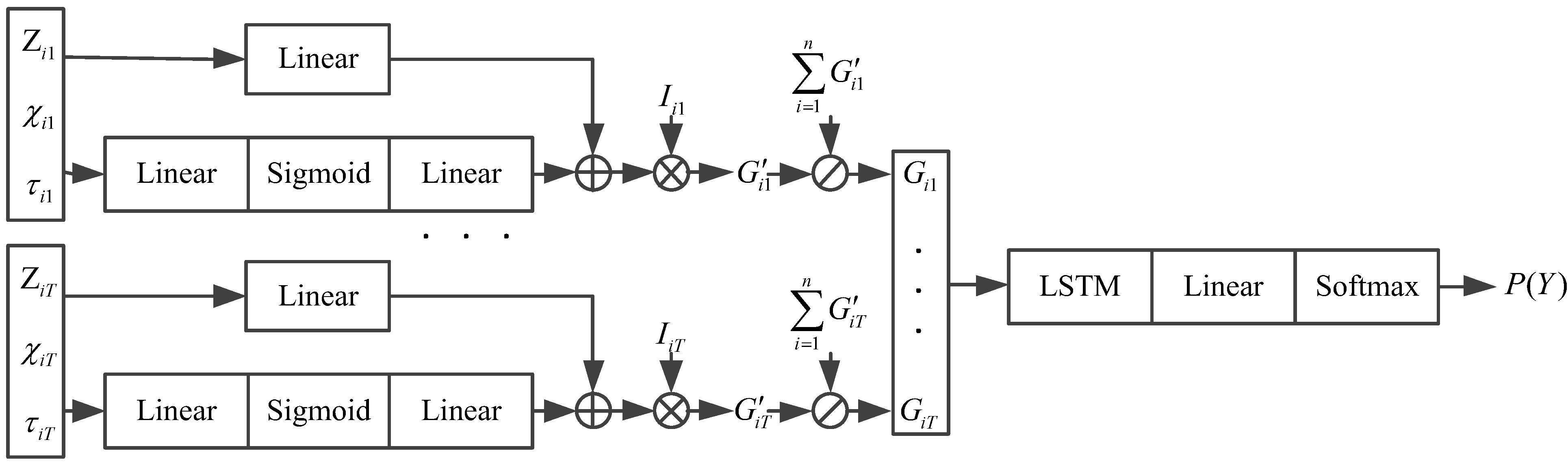
When trajectory prediction is achieved by the integral-iteration method, the initial state of integration has a great influence on the prediction precision. As can been seen from Figure 1, The original data and observation data are brought into the initial and last state modification network, which is designed to modify the initial and last state of observation data, in order to generate a more accurate initial and last state. The LSTM network with a size of $[6,128,2]$, and the fully connected network with a size of $[128,6]$ are used for training. The observed normalized 6-dimensional state sequence is brought into the LSTM network with 128 hidden nodes at 2 layers to learn temporal relationship, and then it is integrated into the fully connected network for dimensionality reduction, which is used to obtain the state of modified initial and last state, $S_i$ and $S_l$, respectively. The structure is shown in Figure 2.

3.2. Parameter Modification Network ${\phi }_m(\cdot )$

Due to the error of the filtering algorithm, the variation of control parameters is not smooth and is fluctuant. Direct estimation using filtering control parameters may lead to a large prediction error. Therefore, the parameter modification network into which the original data and filtering data are brought is designed to modify and smooth the variation of control parameters. The LSTM network, with a size of $[3,128,2]$ and the fully connected network with a size of $[128,6]$, are used for training. The normalized control parameters after filtering $K_D^{\mathrm{f}},{\beta }^f,K_L^f$ are brought into the network for training, and the modified control parameters $K_D^m,{\beta }^m,K_L^m$ are obtained. The network is shown in Figure 2a.

3.3. Parameter Value Prediction Network ${\phi }_p(\cdot )$

This network is designed to learn the temporal characteristic from the truth control parameter value data, through which the variation of future control parameter values can be predicted. The truth control value data of observation and prediction are brought into the network to learn temporal relationships between them. The LSTM network, with a size of $[3,128,2]$, and the fully connected network with a size of $[128,6]$, are used for training to obtain the predicted control parameter values $K_D^p,\left|{\beta }^p\right|,K_L^p$. The network is shown in Figure 2b.

Based on the common guidance logic of reentry glide target with the purpose of attacking strategic places, it can be usually divided into two parts of longitudinal and lateral guidance. As can be seen from Equation (2), the control parameters $K_D$ and $K_L$ are related to the attack angle of the target, the variation of which are usually smooth, similar to the variation of bank angle $\left|\beta \right|$ value. Therefore, taking the control parameter values $K_D$,$K_L$ and $\left|\beta \right|$, the longitudinal guidance logic of the target can be obtained. On the other hand, the lateral guidance logic decided by the sign of bank angle $sgn(\beta )$ varies with the design, which is difficult to effectively predict. Aimed at this problem, inferring the attack intention of target can be a valid method to obtain a more accurate trajectory. To realize the intention inference, the characteristic of strategic places and the functional relationship between strategic places and trajectories should be analyzed.

4. Importance Map of Strategic Places and the Association Model between Strategic Places and Trajectories

According to the analysis of the guidance mechanism of the target [27], there are strategic places to be attacked. The effective analysis of the situation relationship between target and strategic places and inferring the intention of target can provide more prior information for the prediction of target trajectory. To analyze the attack intention of the reentry glide target, the importance map of strategic places is firstly modeled.

4.1. Importance Map of Strategic Places

Usually, strategic places occupy an area. To accurately describe this area, it is assumed that the mapping area of a strategic place is elliptic in several directions, and its probability distribution conforms to the joint two-dimensional Gaussian distribution, which can be expressed as

$$f_k\left(x,y\right)~N(x_c^k,{\delta }_{1k}^2,y_c^k,{\delta }_{2k}^2,\rho )$$

(4)

where $f_k\left(x,y\right)$ represents the probability density of position $(x,y)$ for the $k-th$ strategic place, $\left(x_c^k,y_c^k\right)$ is the central position of the $k-th$ strategic place’s ellipse, ${\delta }_1,{\delta }_2$ represent the variance of the distribution, and $\rho$ is the correlation coefficient between $x,y$.

According to the theory of two-dimensional normal distribution, assuming that the central position of the distribution is $\left(x_c,y_c\right)$, the rotation angle of mapping ellipse is $\delta$, and the radius of the major and minor axis of the ellipse’s mapping standard deviation are $t_1,t_2$, respectively. Then, the distribution density can be expressed as

$$f(x,y)\sim N\left(x_c,{\sigma }_1,y_c,{\sigma }_2,{\rho }_{xy}\right)=-\exp \left(-\frac{1}{2(1-{\rho }_{xy}^2)}{t}_{xy}\right)/2\pi {\sigma }_1{\sigma }_2\sqrt{1-{\rho }_{xy}^2}$$

(5)

where, ${\rho }_{\mathrm{x}y}=(t_2^2-t_1^2)\cos \delta \sin \delta /\sqrt{{\sigma }_1{\sigma }_2}$ ${\sigma }_1=\sqrt{t_1^2{\cos }^2\delta +t_2^2{\sin }^2\delta }$, ${\sigma }_2=\sqrt{t_2^2{\cos }^2\delta +t_1^2{\sin }^2\delta }$,.$t_{xy}={\left(x-x_c\right)}^2/{\sigma }_1^2-2{\rho }_{xy}\left(x-x_c\right)\left(y-y_c\right)/{\sigma }_1{\sigma }_2+{\left(y-y_c\right)}^2/{\sigma }_2^2$.

According to the absolute importance of each strategic place ${\pi }_k$, considering the combined effect for the location’s importance in the map, the importance of each position in the map is calculated based on the Gaussian mixture model (GMM),

$$p(x,y)={\displaystyle \sum _{i=1}^K{\pi }_i{f}_i(x,y)}$$

(6)

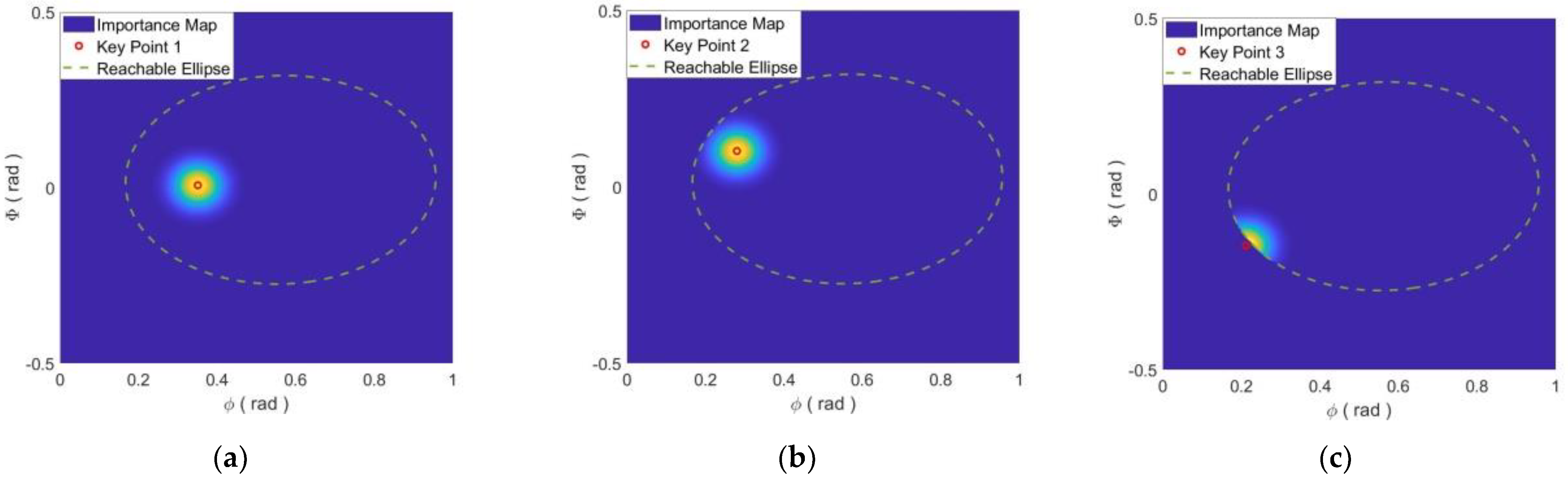
The extreme points of mixing probability are considered the key points attacked by the target. The distribution of probability density can be shown through the heat map, which means the absolute importance of each position and is named as importance map. Compared with the representation by simple points, the importance map can describe the importance of strategic places in more detail and rationality. What is more, based on the proposed model, the comprehensive influence of all strategic places on each position can be obtained that may generate a new key point. As shown in the following three examples, the importance distributions of the strategic places calculated by the importance map are shown in Figure 3.

As can be seen from Figure 3, for the importance map with three strategic places, there are three kinds of cases. The first is that no new key points are generated and the attack positions are the centre of each strategic place, as shown in Figure 3a. The second is that a new key point is generated due to the influence of the two strategic places, as shown in Figure 3b. What is more, the new generated key point should also be considered when inferring the intention of the target. The third is that a new key point is generated by the joint influence of all the strategic places, as shown in Figure 3c.

4.2. Association Models between Strategic Places and Trajectory

4.2.1. Model Setting

In general, the guidance methods of the reentry glide target can be divided into nominal ballistic guidance and predictor–corrector guidance. The nominal trajectory is usually designed by several optimization algorithms when nominal ballistic guidance is used, so that the target could choose the fastest and safest trajectory to attack the key point. When predictor–corrector guidance is adopted, the guidance trajectory can be obtained based on avoid logic for no-fly zones and guidance logic. Therefore, the analysis of the possible trajectories of targets based on strategic places’ distribution and no-fly zone information is of great significance for trajectory prediction.

According to the analysis in Section 3, the lateral guidance is mainly decided by bank angle. Thus, based on the parameter value prediction network in Section 3, the future control parameters $K_L$ and $K_D$ can be obtained. Subsequently, bank angle selects a constants value within $\left[-\pi /2,\pi /2\right]$ according to a certain step, based on the control parameter model, and several predicted trajectories can be obtained when the setting terminal height $h_f$ is reached. Then, the reach region of target and the association trajectories of each key point can be obtained. The model is shown as Figure 4.

As shown in the Figure 4, analyzing the key points within the reach region, the relationship between the position of the target, no-fly zones and key points should be discussed. It is assumed that the radius of no-fly zones is $R_b$. The mapping area of no-fly zone is named no-fly zone mapping corridor, which is between the trajectories generated with a constant bank angle and tangent to the no-fly zone circle. If the key point is within the mapping corridor and sheltered by the no-fly zone, the bank angle needs to be adjusted to avoid the no-fly zone. Otherwise, the trajectory can join the target and key point directly keeping the constant bank angle, such as key point a. For the key points located in the mapping corridor, such as key points b and c, it is necessary to obtain the trajectory and position tangent to the no-fly zone circle. It is generally thought that the less maneuvering operations the target performs, the more energy it can save, so the tangent trajectories can be seen as the approximate trajectory. If the lift of the target is sufficient, based on the Dubbins circle, the turning circle radius of the target is $r_t=R_b$, and the acceleration of tuning satisfies

$$a_t=K_L\rho V^2\sin \left|\beta \right|=\frac{V^2{\cos }^2\theta }{R_b}$$

(7)

In general, the flight path angle is a small value; if the target can fly-around the no-fly zones, it satisfies $\left|{(R_b\rho K_L)}^{-1}\right|\le 1$.

After flying-around, the target flies directly to the key point b. If Equation (7) is not satisfied, the minimal radius of flying-around circle will be $r_t=1/\left|\rho K_L\right|$. Based on the tangent point position, the new flying-around trajectory is obtained, and the whole trajectory is completed. Through the association model, the simple association trajectory between key points and target can be generated, and the time-to-go can be approximately estimated as a key factor to analyze the intention of the target.

4.2.2. Realization Method

(1)

Calculation of reach region.

In order to calculate the reach region, the modified last state in Section 3 is taken as the initial state of integration of trajectories. According to the prediction control parameter $K_{Dp},K_{Lp}$ based on the parameter value prediction network, the constant bank angle is combined, which selects a value uniformly within $\left[-\pi /2,\pi /2\right]$ at a fixed step size. Let the setting height as the terminal condition, then a bunch of trajectories is obtained when the lateral position and reaching time of terminal state are recorded. The projection position of the reachable region is shown in Figure 5a.

In order to determine whether the target is within the reachable region, the lateral position is fitted with ellipse function $A{\varphi }^2+B\varphi \phi +C{\phi }^2+D\varphi +E\phi +F=0$ when $A>0$. Assuming that the position of $i-th$ key point is $[{\varphi }_i,{\phi }_i]$, if $A{\varphi }_i^2+B{\varphi }_i{\phi }_i+C{\phi }_i^2+D{\varphi }_i+E{\phi }_i+F<0$, it means that the key point is within reachable region, and the time-to-go needs to be estimated, while if $A{\varphi }_i^2+B{\varphi }_i{\phi }_i+C{\phi }_i^2+D{\varphi }_i+E{\phi }_i+F<0$, the time-to-go is setting to infinity.

Moreover, as can be seen from Figure 5b, by connecting the lateral position of different trajectories at the same time, the bank angle-time grid can be obtained, which is useful to calculate the bank angle for the key points ${\beta }_k$ and mapping corridor of no-fly zones.

(2)

Calculation of the bank angle and time-to-go for key points.

Obtain the nearest grid position to the key point within the reachable region $[{\varphi }_{b,t}^{\prime },{\phi }_{b,t}^{\prime }]$, and compare the distance between $[{\varphi }_{b,t}^{\prime },{\phi }_{b,t}^{\prime }]$ and key point position with $[{\varphi }_{b-1,t}^{\prime },{\phi }_{b-1,t}^{\prime }]$, $[{\varphi }_{b+1,t}^{\prime },{\phi }_{b+1,t}^{\prime }]$, $[{\varphi }_{b,t+1}^{\prime },{\phi }_{b,t+1}^{\prime }]$ and $[{\varphi }_{b,t-1}^{\prime },{\phi }_{b,t-1}^{\prime }]$, by which the grid position key point location can be determined. Then, through interpolation, the bank angle of key point can be obtained, and the time of nearest grid position $t$ can be seen as the time-to-go of key point $t_{\mathrm{t}}$.

(3)

Calculation of mapping corridor of no-fly zones.

The influence of no-fly zones should be considered when the centre of no-fly zones is within the reachable region. Calculate the minimum distance $d_{\beta i}$ and the corresponding time $t_{\beta i}$ between the trajectories of each bank angle $X_{\beta i}$ and the centre of no-fly zones, where $i=1:N$, and $N$ is the number of setting bank angle. Then, assuming that the distance between trajectories and no-fly zones is $\Delta d$, $\Delta d_i=R_b-d_{\beta i}$. The $\left(p-1\right)-th$ and $p-th$ trajectories that satisfy $\Delta d_{p-1}\Delta d_p<0$ are selected to estimate the bank angle of tangent trajectory for no-fly zones ${\beta }_b$.

$${\beta }_b=\frac{\left|\Delta d_{p-1}\right|{\beta }_p+\left|\Delta d_p\right|{\beta }_{p-1}}{\left|\Delta d_p\right|+\left|\Delta d_{p-1}\right|}$$

(8)

The estimated tangent time is $t_{\beta b}$, which represents the time when the trajectory of ${\beta }_b$ is closest to the no-fly zones.

The relationship between the no-fly zone and the reachable region can be divided into full inclusion and partial inclusion. When one boundary of the no-fly zone is out of the reachable zone, as shown in Figure 6a,c, the tangent point on one side should be discussed. When the no-fly zone and the reachable zone are shown in Figure 6b, the positions of tangential points on both sides of the no-fly zone need to be determined. The corridor condition can be expressed as

$$\left\{\begin{array}{l}{\beta }_k\le {\beta }_{br}, if t_t\ge t_{\beta r}\\ {\beta }_l\le {\beta }_k\le {\beta }_r, if t_t\ge \min (t_{\beta l,}{t}_{\beta r})\\ {\beta }_k\le {\beta }_l, if t_t\ge \min (t_{\beta l,}{t}_{\beta r})\end{array}\right.$$

(9)

where ${\beta }_r$ is the bank angle of a trajectory that is tangent to the no-fly zones from the right, and ${\beta }_l$ is the bank angle of a trajectory which is tangent to the no-fly zones from the left. The parameters $t_{\beta l,}{t}_{\beta r}$ represent the tangent time from the right and left, respectively.

(4)

Estimation of time-to-go for key points within mapping corridor.

If the key points are within the mapping corridor, the time-to-go of key points should be refreshed. According to step (3), the trajectory of bank angle ${\beta }_b$ that integrates to time $t_{\beta b}$ can be obtained. If the heading deviation angle $\left|\Delta {\psi }_k\right|$ between the target at this time and key point k is less than the setting threshold value $\left|{\epsilon }_{\psi }\right|$, setting the bank angle as $\beta =0$, let the target fly to the key point. Otherwise, $\left|\Delta \psi \right|\ge {\epsilon }_{\psi }$, the change law of bank angle is according to the following flying around rule,

$${\beta }_t=\left\{\begin{array}{l}\mathrm{sgn}(\Delta {\psi }_k)\arcsin \left(\left|{\left(r_b\rho K_{Lt}\right)}^{-1}\right|\right),if \arcsin \left(\left|{\left(r_b\rho K_{Lt}\right)}^{-1}\right|\right)\le 1\\ \pi \mathrm{sgn}(\Delta {\psi }_k)/2, if \arcsin \left(\left|{\left(r_b\rho K_{Lt}\right)}^{-1}\right|\right)>1\end{array}\right.$$

(10)

Stop flying around until $\left|\Delta {\psi }_k\right|<{\epsilon }_{\psi }$, and record the cost time of flying around $t_c$. Then, set the bank angle equal to 0 l, let the target fly to the key point until the distance between the target and key point $d<{\epsilon }_d$, and record the cost time $t_d$. Therefore, the time-to-go of the target for key points with the mapping corridor of no-fly zones is refreshed as $t_t=t_{\beta b}+t_c+t_d$.

On the other hand, when the key point is out of the reachable region, the time-to-go for the key point will be $t_f=\infty$.

The dynamic effects are shown in Figure 7, where (a), (b), (c) and (d) represent the change process of dynamic association trajectories for different key points. The blue shaded area represents the no-fly zone mapping corridor, the gray shaded area represents the no-fly zones, and the blue dotted line represents the associated trajectory between the target and the key points.

It can be seen that, based on the proposed model, the approximate lateral trajectories for key points can be obtained quickly, which can be used for the simple calculation of the time-to-go of the target. Some key points will gradually leave the target’s reachable region, and their time-to-go reaches infinity. The proposed model can provide more auxiliary information for the later analysis of the attack intention of the target.

5. Intelligent Trajectory Prediction Algorithm Based on Intention Inference

According to the importance map and association trajectories model in Section 4, the intention information of the target could be obtained effectively. The method to predict trajectories based on intention inference is proposed in this section.

5.1. Factors Influencing the Target Threat Value

Since the target may adopt different lateral guidance logic and avoid methods, the lateral guidance law of the target does not change completely as the threat value increases. The trajectory of the target may not meet the Markov process, such as the predictor–corrector guidance algorithm. Aimed at this problem, several influencing factors related to the threat value should be analyzed according to the observation data, and it should be determined which key point is the attack position of the target. What is more, the attack process is a guidance process of reentry glide targets. Referring to the common guidance methods of reentry targets [23], the prediction of target attack intention is realized from the guidance theory. In this paper, the cross-range, longitudinal range, time-to-go and relative importance of different strategic places are selected as influencing factors to evaluate the threat value of targets.

(1)

Analysis of the influence of cross-range.

According to the analysis of lateral guidance logic, the cross-range between the target and key points [28] can effectively reflect the lateral guidance effect of the target. The formula of cross-range is as follows:

$${\chi }_i=\mathrm{arc}\sin \left(\sin \left(S_{fi}\right)\sin (\Delta {\psi }_i)\right)$$

(11)

where ${\chi }_i,S_{fi},\Delta {\psi }_i$ respectively represent the cross-range, range-to-go and flight heading deviation angle of $i-th$ key point. Furthermore, $S_{ft}=\arccos \left(\cos {\phi }_f\cos \phi \cos ({\varphi }_f-\varphi )+\sin {\phi }_f\sin \phi \right)$, ${\psi }_f=\mathrm{arc}\sin \left(\sin ({\varphi }_f-\varphi )\cos \phi /\sin \left(S_{togo\_f}\right)\right)$, $\Delta {\psi }_f=\psi -{\psi }_f$. In general, the cross-range is smaller, the threat value of the target for the key point is higher, and the threat value is inversely proportional to the cross-range.

(2)

Analysis of the influence of longitudinal range

In order to analyze the longitudinal guidance of the target, the flight height should decrease as the range-to-go decreases. To reflect the longitudinal effect, the longitudinal range of $i-th$ key point at time $t$ is defined as

$$Z_{i,t}=\left\{\begin{array}{l}{H}_t/\sin \left(S_{fi,t}\right),if 0<Z_{i,1,\dots t-1}<1\\ 0,if Z_{i,1\dots t-1}\ge 1 \mathrm{or} Z_{i,1\dots t-1}=0\end{array}\right.$$

(12)

Generally, if the target intends to attack the key point, the longitudinal range should increase gradually to close to 1. When the range-to-go is less than the flight height in the observation flight trajectory, it means that the target has crossed the center of strategic places, and the threat value of this key point decreases to 0 immediately. Therefore, when $Z<1$, the longitudinal range is higher, the threat value is higher, and it is proportional to the longitudinal range.

(3)

Analysis of time-to-go.

For the convenience of analysis, the time-to-go calculated through the trajectories association model in Section 4 is nondimensionalized; ${\tau }_{fi}=t_{f_i}\sqrt{g_0/R_e}$. The time-to-go is smaller, the threat value is higher and it is inversely proportional to the time-to-go.

(4)

Analysis of relative importance.

According to the analysis of the importance map of the target in Section 4.1, when the reachable region of the target changes, the relative importance of each strategic place is calculated as follows:

$$I_i^{\prime }=\left\{\begin{array}{l}{\displaystyle \underset{\Omega }{\iint }{\pi }_{{}_i}{f}_i(\varphi ,\phi )d_{\varphi }{d}_{\phi }}/{\displaystyle \sum _{i=1}^n{\displaystyle \underset{\Omega }{\iint }{\pi }_{{}_i}{f}_i(\varphi ,\phi )d_{\varphi }{d}_{\phi }}},if \mathrm{key} \mathrm{point} \mathrm{is} \mathrm{the} \mathrm{center} \mathrm{of} \mathrm{strategic} \mathrm{place}\\ {\displaystyle \sum _{i=1}^q{\displaystyle \underset{\Omega }{\iint }{\pi }_{{}_i}{f}_i(\varphi ,\phi )d_{\varphi }{d}_{\phi }}}/q{\displaystyle \sum _{i=1}^n{\displaystyle \underset{\Omega }{\iint }{\pi }_{{}_i}{f}_i(\varphi ,\phi )d_{\varphi }{d}_{\phi }}},if \mathrm{key} \mathrm{point} \mathrm{is} \mathrm{generated} \mathrm{newly}\end{array}\right.$$

(13)

$$I_i=I_i^{\prime }/{\displaystyle \sum _i^n{I}_i^{\prime }}$$

(14)

where $\mathsf{\Omega }$ represents the predicted reachable region.

According to Equation (13), if the key point is newly generated, its relative importance is the average of the mixture distribution that produces it. The relative importance is higher when the threat value is higher, and the threat value is proportional to the relative importance. The effect is shown in Figure 8. As shown in (a) and (b), the major mapping area of strategic places 1, 2 are within the reachable region, which means that the threat value for key points 1, 2 is higher. Moreover, as shown in (c), the major mapping area of strategic place 3 is not within the reachable region, hence the threat value for key point 3 is low.

According to the above analysis, the threat value function of target for the $i-th$ key point can be defined as

$$G_i\left(x_t\right)=\frac{I_i\left(x_t\right)f_Z\left(Z_i\left(x_t\right)\right)f_{\chi }\left(1/{\chi }_i\left(x_t\right)\right)f_{\tau f}\left(1/{\tau }_{fi}\left(x_t\right)\right)}{{\displaystyle \sum _{i=1}^n{I}_i\left(x_t\right)f_Z\left(Z_i\left(x_t\right)\right)f_{\chi }\left(1/{\chi }_i\left(x_t\right)\right)f_{\tau f}\left(1/{\tau }_{fi}\left(x_t\right)\right)}}$$

(15)

where $f_Z$, $f_{\chi }$ and $f_{\tau f}$ represent the function between threat value $G$ and longitudinal range $Z$, cross-range $\chi$, and nondimensional time-to-go ${\tau }_f$, respectively.

Because there is no certain functional form of $f_Z$, $f_{\chi }$ and $f_{\tau f}$, by combining the nonlinear fully-connected network with LSTM, the intention inference network is designed in this paper.

5.2. Design of Intention Inference Network

Since the functional form of $f_Z$, $f_{\chi }$ and $f_{\tau f}$ cannot be determined, it is designed as a combination of the linear and nonlinear functions. The intention inference is designed as a temporal function related to the threat value

$$p\left(Y\right)=f_G(G_{i1:it})$$

(16)

The network structure is shown in Figure 9. Based on the network shown in Figure 9, the nonlinear term can be added when the original linear relationship is kept. What is more, the function form and weight of influencing factors do not need to be set in advance. The intended key point can be inferred end to end. After training, the threat value can also be calculated and an accurate functional formula can be obtained to calculate the threat value.

5.3. Signal Change Commonly Used in Predictor–Corrector Guidance

(1)

The reentry glide target will fly towards the key point;

(2)

The reentry glide target will avoid the no-fly zone.

Based on these principles, the change logic of bank angle is shown in Figure 10. When the trajectory of the target is extrapolated and the direction of flight heading angle does not pass through the no-fly zone, as shown in Figure 10a, the change rule of the target will be as follows:

$$\mathrm{sgn}(\beta )=\mathrm{sgn}(\Delta \psi )=\mathrm{sgn}({\psi }_t-\psi )$$

(17)

According to Equation (17), the sign of bank angle is predicted to fly toward the key point. If the direction of the flight heading angle passes through the no-fly zone as shown in Figure 10b, the variation rule is

$$\mathrm{sgn}(\beta )=\mathrm{sgn}(\Delta {\psi }_b)=\mathrm{sgn}({\psi }_b-\psi )$$

(18)

According to Equation (18), the sign of bank angle is predicted to change towards the direction avoiding the no-fly zones the fastest.

5.4. Process of Intelligent Trajectory Prediction Based on Intention Inference

The process of trajectory prediction based on intention inference is shown in Figure 11.

(1)

In order to improve the efficiency of network learning, the observed data are normalized first and then input into the initial and last state modification network to obtain modified initial and last state of observation, which can improve the accuracy of predicted trajectory and modified filtering trajectory;

(2)

Obtain the filtering data $p_f=[K_D^f,\left|{\beta }^f\right|,K_L^f]$ by the trajectory tracking algorithm;

(3)

Input the filter control parameters into the parameter modification network to obtain more accurate filtering control parameters $[K_D^m,{\beta }^m,K_L^m]$;

(4)

Input the value of modified filtering control parameters into the parameter value prediction network, and obtain the predicted control parameter values $[K_D^p,\left|{\beta }^p\right|,K_L^p]$ according to the temporal law of $[K_D^m,\left|{\beta }^m\right|,K_L^m]$;

(5)

Based on the importance map, trajectories association models and others, obtain the influence factors such as cross-range, longitudinal range, time-to-go, and relative importance, then input these factors into the intention inference network, identify the intention of target, and obtain the threat value;

(6)

According to the intention of the target, combine the sign change rule of bank angle with the predicted control parameter value, and extrapolate the predicted trajectory by the integral-iteration method.

5.5. Loss Function of Whole Network

The losses of the whole network include the loss of initial and last state network $l_{il}$, the loss of parameter modification network $l_m$, the loss of parameter value prediction network $l_{vp}$ and the loss of intention inference network $l_{ip}$. The loss function of each network can be expressed as

$$l_{il}=\sqrt{{\displaystyle \sum _i^N{\left(S_{mlli}-S_{olli}\right)}^2}/N}+\sqrt{{\displaystyle \sum _i^N{\left(S_{mili}-S_{oili}\right)}^2}/N}$$

(19)

$$l_m=\sqrt{{\displaystyle \sum _i^N{\left(K_{mi}-K_{fi}\right)}^2}/N}$$

(20)

$$l_p=\sqrt{{\displaystyle \sum _i^N{\left(K_{pi}-K_{di}\right)}^2}/N}$$

(21)

$$l_{ip}=-[l_{ip}\log p_{ip}+(1-l_{ip})\log p_{ip}]$$

(22)

where $S_{mili}$ and $S_{mlli}$ represent the position of the $i-th$ modified start and last state, respectively, in a batch, $S_{oili}$, $S_{olli}$ represent the position of the $i-th$ observed initial and last state, respectively, in a batch; $N$ represents the number of batches in Equation (19); $K_{mi}$ represents the $i-th$ modified control parameters sequence in a batch; $K_{fi}$ represents the $i-th$ filtering control parameters sequence in a batch in Equation (20); $K_{pi}$ represents the $i-th$ modified parameter value sequence in a batch; $K_{di}$ represents the $i-th$ truth parameter value sequence in a batch in Equation (21); $l_{ip},p_{ip}$ represent the one-hot value of intention label and predicted intention, respectively, in Equation (22).

6. Simulation

6.1. Simulation Environment and Related Settings

(1)

Setting of simulation

In this paper, CAV-H [29] is taken as the non-cooperative reentry glide target, and 6825 trajectories are generated according to the lateral guidance logic and no-fly zone avoidance logic in the literature [30]. The IMM-UKF [31] filtering method is used to track the trajectory. The truth trajectories and filtered trajectories are set as training set and testing set, respectively, with the ratio of 4:1. A total of 1403 trajectories are used to test the prediction method. The network training environment is Pytorch-GPU framework, and Matlab software is employed to draw the final results.

(2)

Training conditions

Each network took 100 trajectories as a batch and trained 1000 epochs in total. The optimizer uses the ADAM optimizer, and the training learning rate is 0.001 for the first 10 epochs, which is then adjusted to 0.0001.

(3)

Definition of errors

In this paper, two types of errors commonly used in trajectory prediction are selected: average error of spatial distance (AESD) and maximum error of spatial distance (MESD). The corresponding definitions are expressed as follows:

AESD is the average spatial distance between truth trajectories and predicted trajectories, such as

$$MESD={\displaystyle \sum _i^N{\displaystyle \sum _k^{L_p}\sqrt{{(X_{pk}^i-X_{tk}^i)}^2+{(Y_{pk}^i-Y_{tk}^i)}^2+{(Z_{pk}^i-Z_{tk}^i)}^2}}}/N$$

(23)

MESD is the maximum spatial distance between truth trajectories and predicted trajectories, such as

$$MESD={\displaystyle \sum _i^N\underset{k}{\overset{L_p}{\max }}\sqrt{{(X_{pk}^i-X_{tk}^i)}^2+{(Y_{pk}^i-Y_{tk}^i)}^2+{(Z_{pk}^i-Z_{tk}^i)}^2}}/N$$

(24)

where $N$ represents the number of the testing dataset trajectories; $L_p$ represents the length of the predicted temporal sequence; $\left[X_{pk}^i,Y_{pk}^i,Z_{pk}^i\right]$ represents the predicted position at the time $k$ of the $i–\mathrm{th}$ test trajectory, and $\left[X_{tk}^i,Y_{tk}^i,Z_{tk}^i\right]$ represents the true position.

6.2. Prediction Effect of Parameter Value Prediction Network

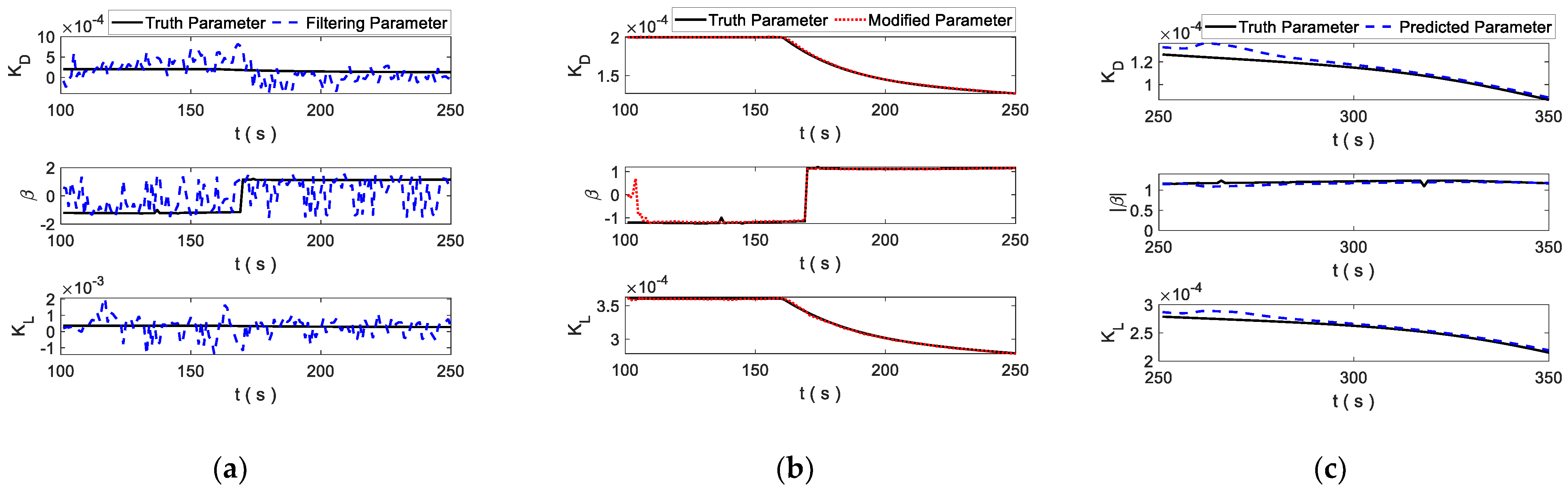
The modification effect of the parameter modification network is shown in Figure 12a. After the filtering of parameters, the control parameters still have great fluctuations and may lead to large errors in parameter fitting and prediction. As shown in Figure 12b, after the parameter modification network, the modified control parameters are relatively close to the truth value. It can be seen from Figure 12c that, based on the modified control parameters, the prediction effect of the control parameter value is close to the truth value, and it can help to more accurately integrate trajectories by iteration.

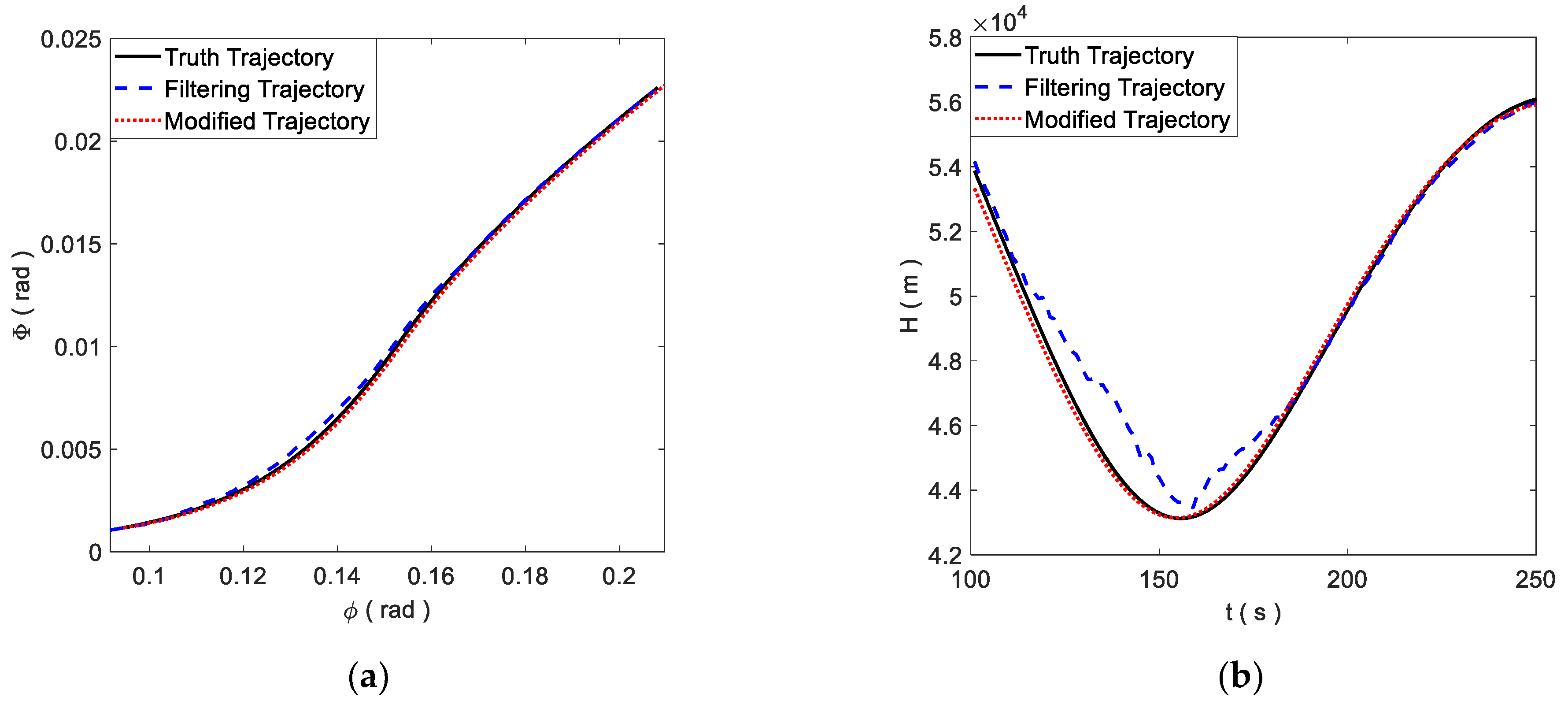
The modification effect of lateral and longitudinal filter trajectories is shown in Figure 13. As can be seen from Figure 13a,b, before modification, both the lateral and longitudinal tracking trajectories of the target have large tracking errors. However, after parameter correction, the modified trajectory of the observation is closer to the truth trajectory than the tracking trajectory. Since the initial state and filtering control parameters are modified by the initial and last state modification network and parameter modification network, it makes the modified filtering trajectory generated by the integration more accurate, which is of great significance for the accurate analysis of influence factors. This method improves the precision of the intention inference and the accuracy of trajectory prediction.

6.3. Influence Factors of Intention and Inference Effects

Based on the intention inference network in Section 5, the change of influence factors and threat value case 1 are as shown in Figure 14, in which the intent key point is key point 1. The relationship among the modified filtering trajectory, the key points, and the no-fly zones are shown in Figure 14a. As can be seen from Figure 14c–f, the time-to-go of the intent key point is relatively small, the cross-range is close to 0, while the longitudinal range gradually rises. The relative influence also changes as time goes on. The importance of the key point c decreases rapidly as it leaves the reachable region of the target, and its threat value also decreases rapidly, as shown in (f). As can be seen in (b), the threat value can be calculated through the intention inference network. The threat value of key point 1 rises over time and is higher than other key points, which finally leads to the accurate prediction of intention inference.

When evaluating the intention inference network on the testing set, the accuracy of intention inference can reach 98.7%, and it can only reach 87.3% referring to the design function in the literature [15].

6.4. Validity Analysis of Trajectory Prediction

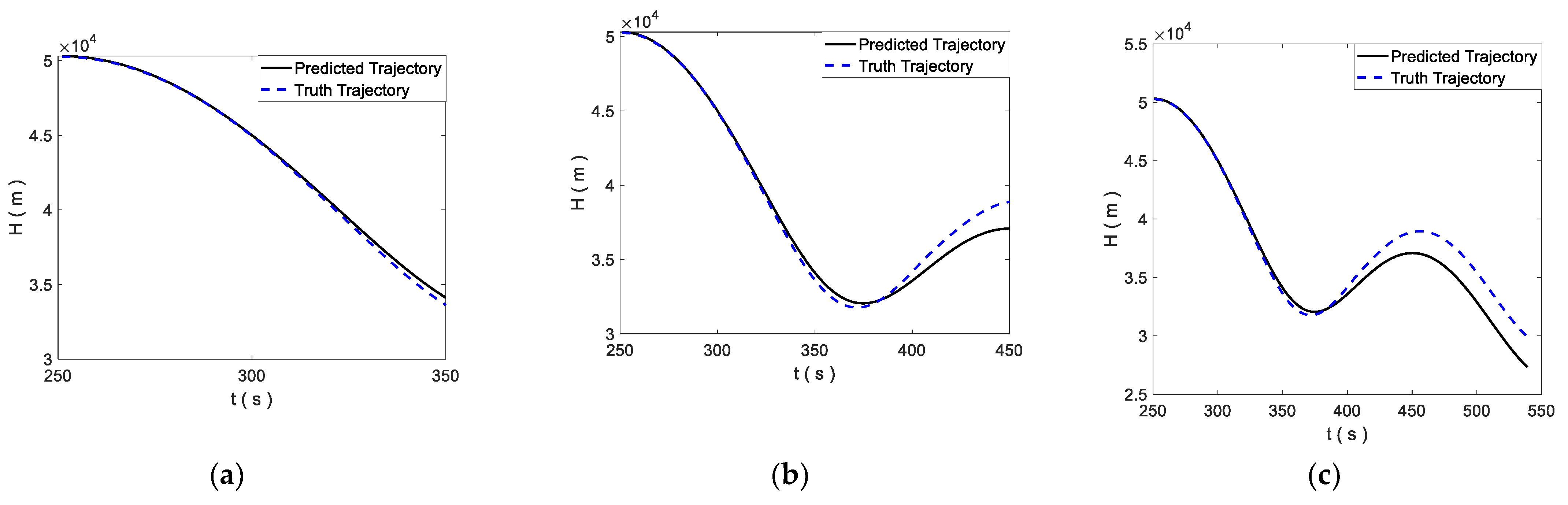
In order to illustrate the effectiveness of the proposed method, two cases of trajectory prediction with different no-fly zone situations are selected in this paper. The first is the target flying around the no-fly zones, while the second is the target flying through between the no-fly zones. With an observation time of 150 s, the predicted trajectories are obtained with 100 s, 200 s and 300 s prediction time. Cases 1 and 2 represent the truth trajectories of flying around and passing through, respectively. The prediction effect of case 1 is shown in Figure 15 and Figure 16, while the prediction effect of case 2 is shown in Figure 17 and Figure 18.

As can be seen from Figure 15, when the prediction time is short, the prediction accuracy is very high. Meanwhile, when the prediction time is longer, the accuracy gradually decreases, which is caused by the accumulation of longitudinal trajectory errors generated by integration. As can be seen from Figure 16, according to the case that the target flies around the no-fly zones, the predicted trajectories based on intention inference in the early stage are more accurate. Because the proposed sign change rule is different from truth guidance logic, as the prediction time increases, the lateral prediction effect may become poor. However, for the long-term trajectory prediction, based on the correct intention inference, lateral prediction error will not spread rapidly, and the prediction effect may become better.

As can be seen from Figure 17, the variation of longitudinal guidance precision in case 2 is similar to that in case 1, which agrees with the longitudinal guidance variation law of the reentry glide target, that is, longitudinal range is mainly related to the control parameter value. However, as can be seen from Figure 19, the flying through predicted trajectory using the intention inference method has a good effect on short-term and long-term prediction. What is more, for long-term prediction, when intentions are accurately judged, lateral prediction errors do not diverge rapidly, and the prediction error increases slowly. Compared with case 1, the lateral predicted trajectory in case 2 is more accurate. On the other hand, it can be seen from Figure 15 and Figure 17 that, after using the parameter value prediction network, the long-term longitudinal integration error of the target still has a high accuracy for the skip trajectory, and the error can be controlled within 500 m. To further demonstrate the accuracy of the prediction method, the overall test results are analyzed in Section 6.5.

6.5. Error Analysis of the Proposed Method

The longitudinal prediction error, lateral prediction error and total error within 100 s, 200 s and 300 s are shown in Figure 19. It can be seen that, in the early period of prediction, the error of the target is very small while the time is less than 80 s. However, due to the difference between the sign change rules and the real guidance logic, the lateral error of the target gradually increases. Since the intention of the target could be correctly predicted by the intention inference network, the lateral error increases slowly within 200 s and 300 s. The longitudinal error increases with time due to the accumulation of the error. The error results are shown in

Table 1. Prediction effect within different prediction times.

Prediction Time	Index	Longitudinal Error	Lateral Error	Whole Error
100 s	AESD(m)	197.53	1608.50	1647.70
	MESD(m)	424.52	8889.49	8918.06
200 s	AESD(m)	554.75	6503.50	6584.09
	MESD(m)	2081.72	18,374.25	18,416.55
300 s	AESD(m)	1296.75	10,505.79	10,662.39
	MESD(m)	3401.00	31,747.06	31,907.31

. Our method obtains the result that the whole error is less than 9 km with a 100 s prediction time and it is less than 32 km with a 300 s prediction time, which shows a good effect on both short and long-term prediction accuracy.

6.6. Comparison with Other Prediction Methods

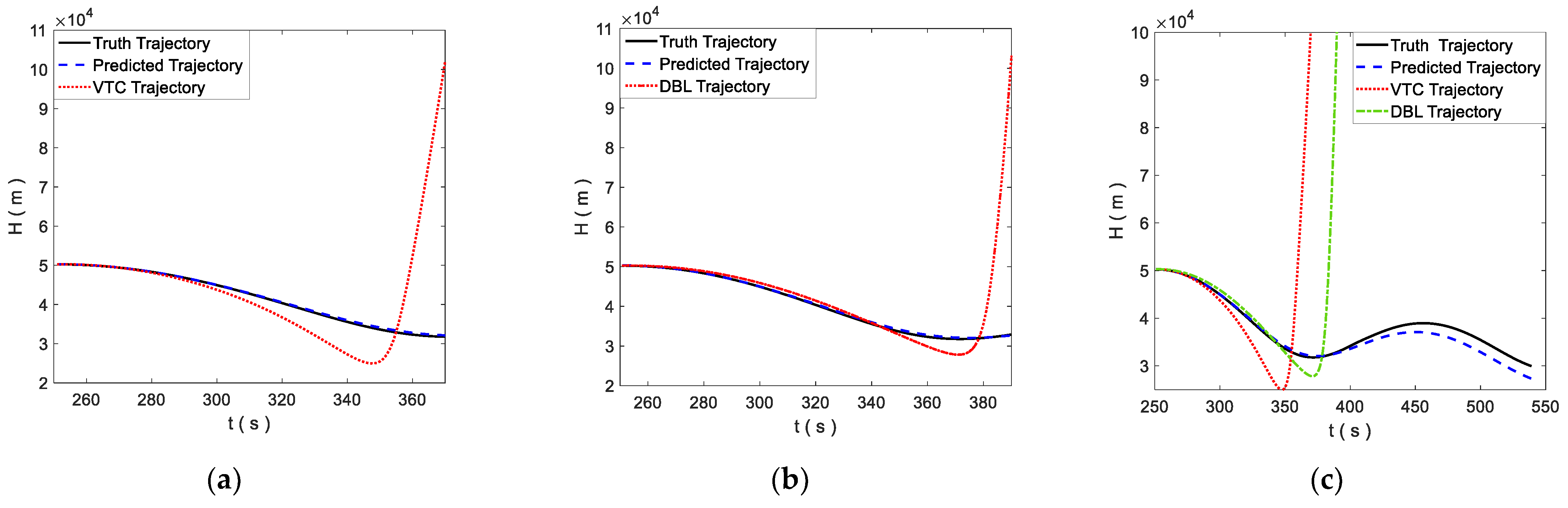
In order to demonstrate the effectiveness of the proposed method further, the proposed method was compared with prediction methods in literature [5,6] with the same condition as in case 1, and the prediction results less than 100 s are shown in Figure 20. The prediction method of literature [5] is named the VTC prediction method, and the prediction method of literature [6] is named the DBL prediction method in this paper.

As can be seen from Figure 20, for the short-term trajectory prediction, the prediction errors of methods do not diverge. The accuracy of the proposed method is the highest, which is caused by the accurate prediction of the control parameter and utilization of intention information. The prediction method based on control parameter $K_D,\beta ,K_L$ is more accurate than the method based on control parameters ${\xi }_v,{\xi }_t,{\xi }_c$, which means that the control parameters $K_D,\beta ,K_L$ better reflect the guidance mechanism of the target.

The above two prediction methods for comparison rely on parameter fitting; when the extrapolation time by integration is longer than 100 s, the prediction errors of the two methods begin to diverge rapidly, and the divergence effect is shown in Figure 21 and Figure 22. As can be seen from Figure 21a,b due to the imprecise prediction for nonlinear changes of control parameters with the pure fitting of parameters, the prediction error diverges rapidly, especially in the longitudinal direction. For the lateral direction prediction, since pure parameter fitting cannot change the sign of bank angle, the direction of the target’s velocity and the direction of the key point may be reversed, as shown in Figure 22a,c. From long-term trajectory prediction, as shown in Figure 21c and Figure 22c, the proposed method obtains longitudinal prediction results within 300 s without the divergence of error. On the other hand, for the lateral prediction, because of a correct intention inference and sign variation rule of bank angle logic, the lateral long-term trajectory prediction can still maintain high precision. The specific prediction results for 100 s, 150 s and 200 s are shown in

Table 2. Prediction error between different prediction.

Methods	Index	100 s	150 s	200 s
Proposed method	AESD(m)	1647.70	5522.77	6584.09
	MESD(m)	8918.06	17,103.62	18,416.55
VTC prediction method	AESD(m)	23,001.35	—	—
	MESD(m)	101,632.79	—	—
DBL prediction method	AESD(m)	24,620.28	—	—
	MESD(m)	200,958.71	—	—
Reference method	AESD(m)	4231.36	6862.23	10,446.81
	MESD(m)	17,213.44	26,843.11	52,487.36

. Here, the reference method is the prediction method in the literature [18].

Analysis of the prediction results, the proposed method realizes the best results within 100 s, 150 s and 200 s. In particular, because of the valid intention inference, prediction error does not diverge rapidly in the long-term prediction, and it may modify the prediction error. Compared with the method in this paper, the intended method of reference method has a larger fluctuation in the prediction of control parameters, resulting in a larger prediction error. On the other hand, due to the possible non-Markov characteristics of the target’s guidance law, the method in this paper can improve the accuracy of long-term trajectory prediction by slowing down the rapid divergence of prediction error when the sign-changing method is adopted.

In the future work, the key to improve the prediction accuracy of intention trajectory is establish an effective correlation relationship between the target’s intention and the sign variation of bank angle, which is the focus of our future research.

7. Conclusions

In this paper, aimed at the problem of maneuvering mode mutation and insufficient utilization of intention information in trajectory prediction for reentry glide target, an intelligent trajectory prediction algorithm based on intention inference is proposed. According to the guidance method of the target, the prediction process is divided into longitudinal prediction process and lateral prediction process. Firstly, based on the suitable control parameter model and sequential neural network, the initial and last state modification network, parameter modification network and parameter value prediction network are established to realize the prediction of the control parameter value. Secondly, the importance map model is developed based on the Gaussian mixture model. On this basis, the association model between strategic places and trajectories is presented to calculate the related factors of intention. Then, to adaptively calculate the threat value and infer attack intention, the intention inference network is introduced. Combined with the sign variation rule of bank angle, the lateral prediction is realized. Finally, according to the simulation results, the parameter prediction network of this paper has an excellent longitudinal prediction effect, the proposed intention parameters reflect good intention characteristics, and the intention network can accurately infer the intention of the target. It is proved that the proposed method can realize accurate and long-term trajectory prediction under different conditions. Compared with other mainstream methods, the prediction accuracy and long-term prediction effect of our method produces the best prediction result

References

- Xie, Y.; Liu, L.; Tang, G.; Zheng, W. A reentry trajectory planning approach satisfying waypoint and no-fly zone constraints. In Proceedings of the 5th International Conference on Recent Advances in Space Technologies-RAST2011, Istanbul, Turkey, 9–11 June 2011; pp. 241–246. [Google Scholar]
- Luo, C.; Lei, H.; Li, J.; Zhou, C. A new adaptive neural control scheme for hypersonic vehicle with actuators multiple constraints. Nonlinear Dyn. 2020, 100, 3529–3553. [Google Scholar] [CrossRef]
- Bu, X.; Qi, Q.; Jiang, B. A Simplified Finite-Time Fuzzy Neural Controller with Prescribed Performance Applied to Waverider Aircraft. IEEE Trans. Fuzzy Syst. 2021, 30, 2529–2537. [Google Scholar] [CrossRef]
- Bu, X.; Jiang, B.; Lei, H. Non-fragile Quantitative Prescribed Performance Control of Waverider Vehicles with Actuator Saturation. IEEE Trans. Aerosp. Electron. Syst. 2022, 58, 3538–3548. [Google Scholar] [CrossRef]
- Zhai, D.L.; Lei, H.M.; Li, J.; Liu, T. Trajectory prediction of hypersonic vehicle based on adaptive IMM. Acta Aeronaut. Et Astronaut. Sin. 2016, 37, 3466–3475. [Google Scholar]
- Li, S.; Lei, H.; Zhou, C. Trajectory Prediction Algorithm for Hypersonic Reentry Glide Target Based on Control Variables Estimation. Syst. Eng. Electron. 2020, 42, 2320–2327. [Google Scholar]
- Han, C.; Xiong, J.; Zhang, K. Method of Trajectory Prediction for Unpowered Gliding Hypersonic Vehicle. Mod. Def. Technol. 2018, 46, 146–151. [Google Scholar]
- Ferreira, L.O. Nonlinear Dynamics and Stability of Hypersonic Reentry Vehicles; University of Michigan: Ann Arbor, MI, USA, 1995. [Google Scholar]
- Chen, X.; Hou, Z.; Liu, J.; Chen, X. Phugoid Dynamic Characteristic of Hypersonic Gliding Vehicles. Sci. China Inf. Sci. 2011, 54, 542–550. [Google Scholar] [CrossRef] [Green Version]
- Vinh, N.X.; Kim, E.K.; Greenwood, D.T. Second-Order Analytical Solutions for Re-entry Trajectories. In Proceedings of the AIAA Atmospheric Flight Mechanic Conference, Monterey, CA, USA, 9–11 August 1993. [Google Scholar]
- Vinh, N.X.; Kuo, Z.S. Improved Matched Asymptotic Solutions for Three-Dimensional Atmospheric Skip Trajectories. In Proceedings of the AIAA/AAS Astrodynamic Conference, San Diego, CA, USA, 29–31 July 1996. [Google Scholar]
- Lu, P. Asymptotic Analysis of Quasi-Equilibrium Glide in Lifting Entry Flight. J. Guid. Control Dyn. 2006, 29, 662–670. [Google Scholar] [CrossRef]
- Zhang, J.; Xiong, J.; Lan, X.; Shen, Y.; Chen, X.; Xi, Q. Trajectory prediction of hypersonic glide vehicle based on SVM and EKF. IEEE Sens. J. 2020, 46, 2094–2105. [Google Scholar]
- Liu, Y.; Li, X.R. Intent Based Trajectory Prediction by Multiple Model Prediction and Smoothing. In Proceedings of the AIAA Guidance, Navigation, and Control Conference, Kissimmee, FL, USA, 5–9 January 2015. [Google Scholar]
- Frontera, G.; Besada, J.A.; López-Leonés, J. Generation of Aircraft Intent Based on a Microstrategy Search Tree. IEEE Trans. Intell. Transp. Syst. 2017, 18, 1405–1421. [Google Scholar] [CrossRef]
- Kai, Z.; Xiong, J. Discussion on Long-Term Trajectory Prediction of Hypersonic Gliding Reentry Vehicle. Tactical Missile Technol. 2018, 4, 13–17. [Google Scholar]
- Kai, Z.; Jiajun, X.; Fan, L.; Ting-Ting, F.U. Bayesian Trajectory Prediction for a Hypersonic Gliding Reentry Vehicle Based on Intent Inference. Yuhang Xuebao/J. Astronaut. 2018, 39, 1258–1265. [Google Scholar]
- Hu, Y.; Gao, C.; Li, J.; Jing, W.; Li, Z. Novel trajectory prediction algorithms for hypersonic gliding vehicles based on maneuver mode on-line identification and intent inference. Meas. Sci. Technol. 2021, 32, 115012. [Google Scholar] [CrossRef]
- Gers, F.A.; Schmidhuber, J.; Cummins, F. Learning to Forget: Continual Prediction with LSTM. Neural Comput. 2000, 12, 2451–2471. [Google Scholar] [CrossRef] [PubMed]
- Zou, Z.; Shi, Z.; Guo, Y.; Ye, J. Object Detection in 20 Years: A Survey. arXiv 2019, arXiv:1905.05055. [Google Scholar]
- Guoqiang, Z.; Lingfang, S.; Xiuyu, Z. Neural Networks Approximator Based Robust Adaptive Controller Design of Hypersonic Flight Vehicles Systems Coupled with Stochastic Disturbance and Dynamic Uncertainties. Math. Probl. Eng. 2017, 2017, 7864375. [Google Scholar]
- Wang, S.; Zhao, P.; Yu, B.; Huang, W.; Liang, H. Vehicle Trajectory Prediction by Knowledge-Driven LSTM Network in Urban Environments. J. Adv. Transp. 2020, 2020, 8894060. [Google Scholar] [CrossRef]
- Cai, Y.; Deng, Y.; Su, Y. LSTM based Trajectory Classification and Prediciton for Hypersonic Vehicle. In Proceedings of the 21st Chinese Coference on System Simulation Technology and Application (CCSSTA21st), Kunming city, China, 26–28 August 2020; Volume 5. [Google Scholar]
- Xie, Y.; Zhuang, X.; Xi, Z.; Chen, H. Dual-Channel and Bidirectional Neural Network for Hypersonic Glide Vehicle Trajectory Prediction. IEEE Access 2021, 9, 92913–92924. [Google Scholar] [CrossRef]
- Zhang, J.; Xiong, J.; Li, L.; Xi, Q.; Chen, X.; Li, F. Motion State Recognition and Trajectory Prediction of Hypersonic Glide Vehicle Based on Deep Learning. IEEE Access 2022, 10, 21095–21108. [Google Scholar] [CrossRef]
- Bartusiak, E.R.; Hao, H.; Jacobs, M.A.; Nguyen, N.X.; Chan, M.W.; Comer, M.L.; Delp, E.J. A Stochastic Grammar Approach to Predict Flight Phases of a Hypersonic Glide Vehicle. In Proceedings of the 2022 IEEE Aerospace Conference (AERO), Big Sky, MT, USA, 5–12 March 2022; pp. 1–15. [Google Scholar] [CrossRef]
- Tian, B.L.; Li, Z.Y.; Wu, S.Y. Reentry trajectory optimization, guidance and control methods for reusable launch vehicles: Review. Acta Aeronaut. Et Astronaut. Sin. 2020, 41, 6–30. [Google Scholar]
- Zhang, K.; Shi, G.X.; Wang, P. Predictor-Corrector Reentry Guidance with Crossrange Dynamic Constraint. J. Astronaut. 2020, 41, 9. [Google Scholar]
- Phillips, T.H. A Common Aero Vehicle (CAV) Model, Description, and Employment Guide. Schafer Corp. AFRL AFSPC 2003, 27, 1–12. [Google Scholar]
- Lin, H.; Du, Y.; Mooij, E.; Liu, W. Improved Predictor-Corrector Guidance with Hybrid Lateral Logic for No-fly Zone Avoidance. In Proceedings of the 2019 International Conference on Control, Automation and Information Sciences (ICCAIS), Chengdu, China, 23–26 October 2019. [Google Scholar]
- Li, S.; Lei, H.; Shao, L.; Xiao, C. Multiple Model Tracking for Hypersonic Gliding Vehicles with Aerodynamic is Modeling and Analysis. IEEE Access 2019, 7, 28011–28018. [Google Scholar] [CrossRef]
Figure 1.
Initial and last modification network.
Figure 2.
The structure of Network: (a) parameter modification network; and (b) parameter value prediction network.
Figure 3.
Effect of Importance map: (a) represents no generated key point; (b) means one key point is generated by two strategic places; and (c) means one key point is generated by all strategic places.
Figure 4.
Association Model between strategic places and trajectories.
Figure 5.
Reachable region and bank angle-time grid: (a) represents the reachable region; (b) represents the bank angle-time grid.
Figure 6.
The relationship between No-fly zones and Reachable region: (a) represents the left boundary of the no-fly zone intersects the reachable region; (b) represents the reachable region fully includes the no-fly zone; (c) represents the right boundary of the no-fly zone intersects the reachable region.
Figure 7.
Association model between key points and trajectories:(a–d) represent the association models at 0 s, 40 s, 90 s and 120 s respectively.
Figure 8.
Relative Importance calculation: (a) is the mapping area key point 1; (b) is the mapping area of key point 2; and (c) is the mapping area of key point 3.