
The Study of Machine Learning Assisted the Design of Selected Composites Properties


Department of Industrial Engineering and Informatics, Faculty of Manufacturing Technologies with a Seat in Prešov, Technical University of Košice, Bayerova 1, 080 01 Prešov, Slovakia
*
Author to whom correspondence should be addressed.
Appl. Sci. 2022, 12(21), 10863; https://0-doi-org.brum.beds.ac.uk/10.3390/app122110863
Submission received: 10 September 2022
/
Revised: 24 October 2022
/
Accepted: 24 October 2022
/
Published: 26 October 2022
(This article belongs to the Special Issue Industry 5.0.: Current Status, Challenges, and New Strategies)
Abstract
:One of the basic points of Industry 5.0 is to make the industry sustainable. There is a need to develop circular processes that reuse, repurpose, and recycle natural resources, and thus, reduce waste. This part can also include composite materials, which were used for some time in many areas. An essential feature of their applicability is the properties of these materials. The ratio of the individual components determines the properties of composite materials, and artificial intelligence machine learning (ML) techniques are already used to determine the optimal ratio. ML can be briefly described as computer science that uses existing data to predict future data. This approach is made possible by the current possibilities of collecting and analysing a large amount of data. It improves the chance of finding more variable influences (predictors) in the processes. These factors can be quantified more objectively; their mutual interactions can be identified, and, thanks to longer-term sampling, their future development behavior can be predictively modelled. The present article deals with the possibility of applying machine learning in predicting the absorption properties of composite material, which consists of a thermoplastic and matrix recycled polyvinyl butyral (PVB), obtained after recycling car glass windshields.
1. Introduction
Industry 5.0 reflects a fundamental shift of companies and economies towards a new paradigm for balancing economic development with solving social and environmental problems [1]. It focuses on three interconnected core values: human-centeredness, sustainability, and resilience (Figure 1).
Industry 5.0 recognizes the power of industry to achieve societal goals, to become a provider of prosperity by making production respect the boundaries of our planet, and to put the well-being of industrial workers at the center of the production process. One of its priorities is environmental protection. Recycling rates are increasing in Europe and the reuse and recycling of discarded products and materials will become a necessity as the shortage of raw materials becomes more pressing. Some materials fit quite easily into the circular economy concept, while others (such as composite materials, fiber-reinforced plastics, metallurgical waste, etc.) present a much more challenging challenge and require further research [2]. The effort is, therefore, in conjunction with intelligent digital technology, artificial intelligence, and big data, to create a more integrated and better-connected ecosystem for companies [3]. Artificial intelligence, as a key element, should significantly contribute to the fulfilment of the goals of Industry 5.0 in all its areas.
The presented contribution points out the possibilities of using artificial intelligence-machine learning (ML) methods in the design of a model for evaluating the absorption properties of selected composite materials.
A composite material is a material that is made from two or more basic materials that have different chemical or physical properties. By combining them, a new material with new properties will be created. Within the structure of the new material, individual elements remain separate and distinct, distinguishing composites from mixtures and solid solutions. Base materials often have distinctly characteristic properties, and the combined architecture built from the base materials allows composites to have unprecedented properties. Recently, ML is seen as a promising tool for designing and discovering new composite materials [4]. This technique was described in [5] where machine learning was applied to a composite system in predicting mechanical properties, including toughness and strength; in [6] ML was used as a tool to develop polymer composites with higher specific strength and stiffness along with higher resistance to impact, wear, and fatigue. The advantage of using ML in model finding for evaluating the properties of composite materials is that using only a subset of the possible data, ML algorithms can uncover hidden patterns in the data and learn an objective function that best maps the input variables to an output variable (or output variables)—a process called the training process [5]. In order to understand the behavior of the process and the interrelationships between input parameters and outputs (reactions) in any process, it is useful to look for suitable models [1,7]. The developed models can also act as effective prediction tools in predicting preliminary response values for given sets of input parameters [1]. Depending on the architecture used, they can sometimes be called deep machine learning. These algorithms use computational methods to “learn” information directly from the data without a predetermined equation as a model [8,9,10].
To find the problem optimal solutions, gain knowledge of the process, or predict the future state are used computer models [9,10], as do many other machine learning algorithms, neural networks work by building a model that we then train on as much labeled data as possible [11]. Based on this known training data, the model learns to “predict” the outcomes of new, unknown cases. A “self-learning” process can create prediction models from the history of time-dependent data. The results obtained by these models are evaluated using tools of modern statistics [12].
2. Work Methodology
The investigated composite materials were subjected to tests in a climatic chamber in order to monitor their absorption capacity. Three samples with different ratios of individual parts of the composite material were examined. Due to the time and financial demands of such an experiment, results were obtained from only two samples. The task was therefore to find a model using machine learning that would predict values for untested material. We will proceed as follows:
- -
- by measuring, we will determine the absorption values of all material samples (VO_20_PVB_80_TF, VO_30_PVB_70_TF and VO_50_PVB_50_TF);
- -
- materials VO_20_PVB_80_TF and VO_50_PVB_50_TF will be tested in a climate chamber;
- -
- using the measured values, we will compile a training set of data in order to design models for the prediction of values for the material VO_30_PVB_70_TF, which is not tested in a climate chamber;
- -
- we will verify the results obtained through models for materials VO_20_PVB_80_TF and VO_50_PVB_50_TF separately by comparing them with their measured values;
- -
- the more favorable of the models will be applied to predict data for the material VO_30_PVB_70_TF.
2.1. Materials and Test Characterization
The composite material comprises a thermoplastic matrix recycled polyvinyl butyral (PVB), obtained after recycling car glass windshields. It is located as an intermediate layer, which has a safety character. The filler was a fabric from 50% to 80% used tyres. The composite material is made of used tyre fabrics and polyvinyl butyral (Figure 2).
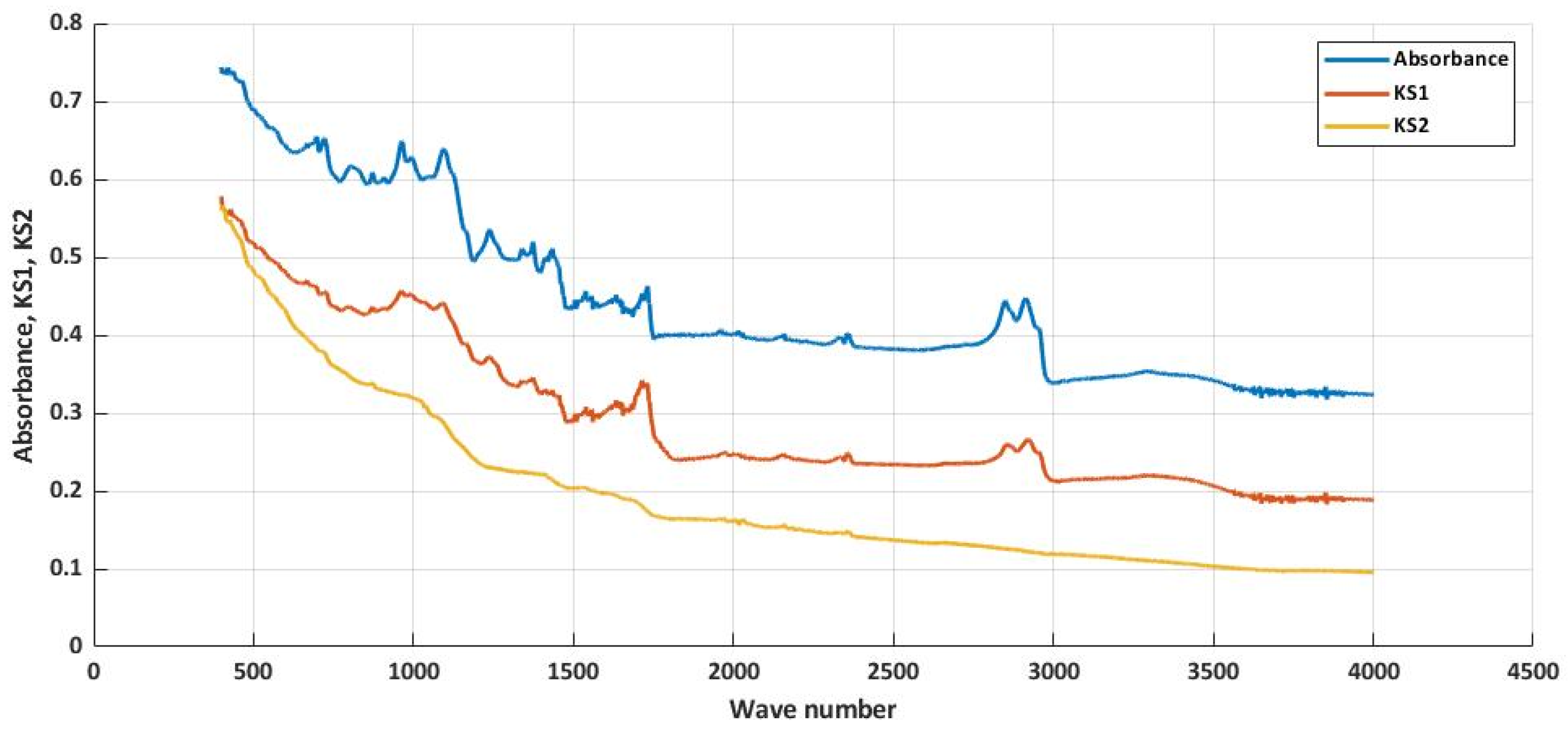
A climate chamber is a device where samples are subjected to ultraviolet radiation, temperatures in minus and values, relative humidity, water treatment (spraying the piece with water), and condensation in certain cycles [13,14,15]. The temperature of the test sample itself depends on the type of material being tested. We tested samples with 50% and 80% fabric when testing the composite material, according to the relevant EN ISO 4892. We selected the mean (50%) and cut-off value (80%) of fabrics in the composite material for testing. The test specimens were exposed to water, temperatures ranging from −50 °C to + 120 °C, UV radiation with a value of 0.76W·m−2·nm−1 and relative humidity. The whole cycle lasted 10 h. In this case, the samples were tested first for seven cycles 70 h and the total exposure time in the climate chamber was 32 cycles, i.e., 320 h. Absorption values (YLabel) for materials VO_20_PVB_80_TF, VO_30_PVB_70_TF, and VO_50_PVB_50_TF were measured using an equipment 620-IR Varian [15]. After the action of the climate chamber on the composite material, it can be seen that the values for certain bundles are different, i.e., that the material’s structure changes during the action of water, ultraviolet radiation, and condensation. The samples were placed in the instrument with a phase textile part to penetrate the transmission transmitted by a sensor mounted on a diamond tip. Subsequently, for the materials VO_20_PVB_80_TF and VO_50_PVB_50_TF, the absorption values after the stay in the climatic chamber were obtained for 70 h (designated KS1) and after 320 h (designated KS2). The number of records for each material was the value 1869 (Figure 3 and Figure 4).
The aim is to find the most advantageous model that would determine the expected values of KS1 and KS2 for individual materials and its use for the material VO_30_PVB_70_TF, whose values we do not know. A training set of values was created to train and find the optimal model, which consisted of a summary of the y-coordinate of the material data, VO_20_PVB_80_TF and VO_50_PVB_50_TF. For optimal use of source data, these were pre-processed into a uniform format to be used in the Matlab environment.
2.2. Methods and Tools Characterization
- Matlab Software Application Tools
Matlab software application tools were used to find the optimal model for the given task. It is a high-performance technical computing language, allowing its robust tools in many research areas [16]. It provides a unified, high-performance environment for working with large data [17]. The basic element is a field not defined by the user, allowing you to solve various technical tasks [9,18]. The wide application of this software is made possible by its so-called toolboxes. Toolboxes are specialized libraries of predefined functions written in the Matlab language, designed to solve problems in a given area. This research article will use the machine learning and deep learning toolbox tools.
- Machine Learning
Machine learning (ML) appeared alongside big data technologies and high-performance computing to create new opportunities to discover, analyze, and understand processes behavior. Methodologies of machine learning typically involve a learning process to learn from “experience” (training data) to perform a task. Machine learning (ML) is used to search for patterns in data files (Figure 5). Their models are important mainly for the decision-making process [11,19]. Numerous ML algorithms were developed for various learning pathways, such as supervised, partially supervised, and unsupervised learning. Guided learning (i.e., predictive modeling) is the most widely used approach in the scientific and engineering fields [10,20].
Supervised learning consists of modeling the relationship between input variables and one or more output variables, which are somewhat dependent on inputs, based on a final set of observations [21]. Deep learning is a subset of machine learning, artificial intelligence, and statistics. It expresses complicated nonlinearity by composing many nonlinear functions [12,22].
- Regression Analysis
In statistics, regression analysis involves processes illustrating the relationships between a dependent variable and one or more independent variables. It is used for two main purposes, i.e., prediction and prediction in machine learning and the development of causal relationships between independent and dependent variables in statistical analysis [14,22]. Gaussian process regression (GPR) combines machine learning tasks, such as model training, uncertainty estimation, and hyperparameter estimation. GPR is a major advantage over other machine learning methods [23]. The GP is a powerful and elegant method with many applications in ML and statistics [24].
- Qualitative Evaluation
Mean square error (MSE), root mean square error (RMSE), mean absolute error (MAE), mean fundamental percentage error (MAPE), and symmetric mean absolute percentage error (SMAPE) are the most popular metrics of predictive models in several areas [23,25].
Coefficient of determination (R2) is commonly used to Evaluate (1) the goodness of the linear fit of regression models in ANNs. A value of 1 means that the regression model explains all the predicted variables, which means that the correlation between the two variables is perfect [25].
Metric-based or square-error metrics are called scale-dependent metrics. They are on the same scale as the original data (2) and provide errors in the same unit [24].
MSE measures the mean square error between the expected and actual values [26,27]. For each data point, the distance is measured vertically from the real value to the corresponding estimated value on the translated line, and the value is multiplied by the second [28]. Subsequently, the sum of all multiplied values is calculated and divided by the number of points.
Percentage-dependent metrics measure error size in rate and provide interpretable thinking about forecast quality (3); the accuracy is usually expressed as a ratio defined by the formula [29]:
MAPE (3) is used as a loss function for regression models in machine learning because it allows a very intuitive explanation of the relative error. These metrics are generally used in practice to determine the accuracy of the developed models
3. Model Proposal
The basis for creating the model will be the source-measured data. Model development will go through different stages such as pre-processing, data training and application of a learning model, and the final model evaluation phase [30]. A more appropriate model will be chosen for the prediction of unknown data. There will be a used deep learning toolbox, which provides a framework for designing and implementing deep neural networks. From this set of tools, regression learner and neural net fitting [31] are used to finding the optimal model. The same set of training data obtained by the measurement is used for these tools. This file will consist of 3738 records. For the needs of neural net fitting, the percentage ratio will be 70:15:15, i.e., for the given values, there will be 2616 values for training, 561 values for testing, and 561 values for validation.
Neural Networks
They are among the modern computational methods used for machine learning. They are usually used where the relationships between inputs and outputs are complex and non-linear. The neural network aims to map a set of numeric inputs to a group of numeric results. The acquired knowledge is ultimately applied to predicting output responses from complex systems [25,32]. The next figure represents the scheme of the fitting neural network in the Matlab environment (Figure 6).
To use this tool, it is necessary to prepare a precisely specified data set. It is required to mark the pumpkin. X-train and y-train form the basis of the training data set.
It gradually works through the individual levels of training set distribution settings, the number of hidden layers (the default number is 10), and the training algorithm selection (Levenberg–Marquardt, Bayesian regularization, and scaled conjugate gradient). In this case, the Levenberg–Marquardt backpropagation algorithm was used [32,33,34]. This algorithm is one of the most popular algorithms in the Matlab toolkit [21]. It is one of the fast algorithms with good performance and is used more than others. The values of the coefficient R2 and MSE are displayed from the qualitative characteristics. If the values do not meet our expectations, we have the opportunity to overtrain the data several times or change other factors affecting these values. After repeated training, we reached the deal R2 = 0.922599. The following scheme shows (Figure 7) the possibility of a graphical representation of the selected model.
R-values measure the correlation between outputs and targets. If the R-value is close to 1, it means a close relationship. From the graphic presentation, we can see that the values of the R coefficient for the training, validation, and test samples show values from 0.89 to 0.922. We can conclude that the model is good. These values were achieved only after retraining the model several times.
The advantage of these tools is that it is possible to generate a function that will be used to predict future values based on this model. In addition, we can create a separate model block for use in the Simulink environment.
After importing the source data, it is possible to use the regression learner tool, which trains regression models for data prediction, without further data preparation. In the environment of the wizard, it will be the predictor, e.g., response [35,36].
In the next step, we select from a set of training algorithms. To find the optimal model as quickly as possible, we search through all algorithms and the system and determine the best model based on qualitative indicators. In this case, it is the GPR algorithm, where the value of R2 is 0.73 (Figure 8).
4. Results and Discussion
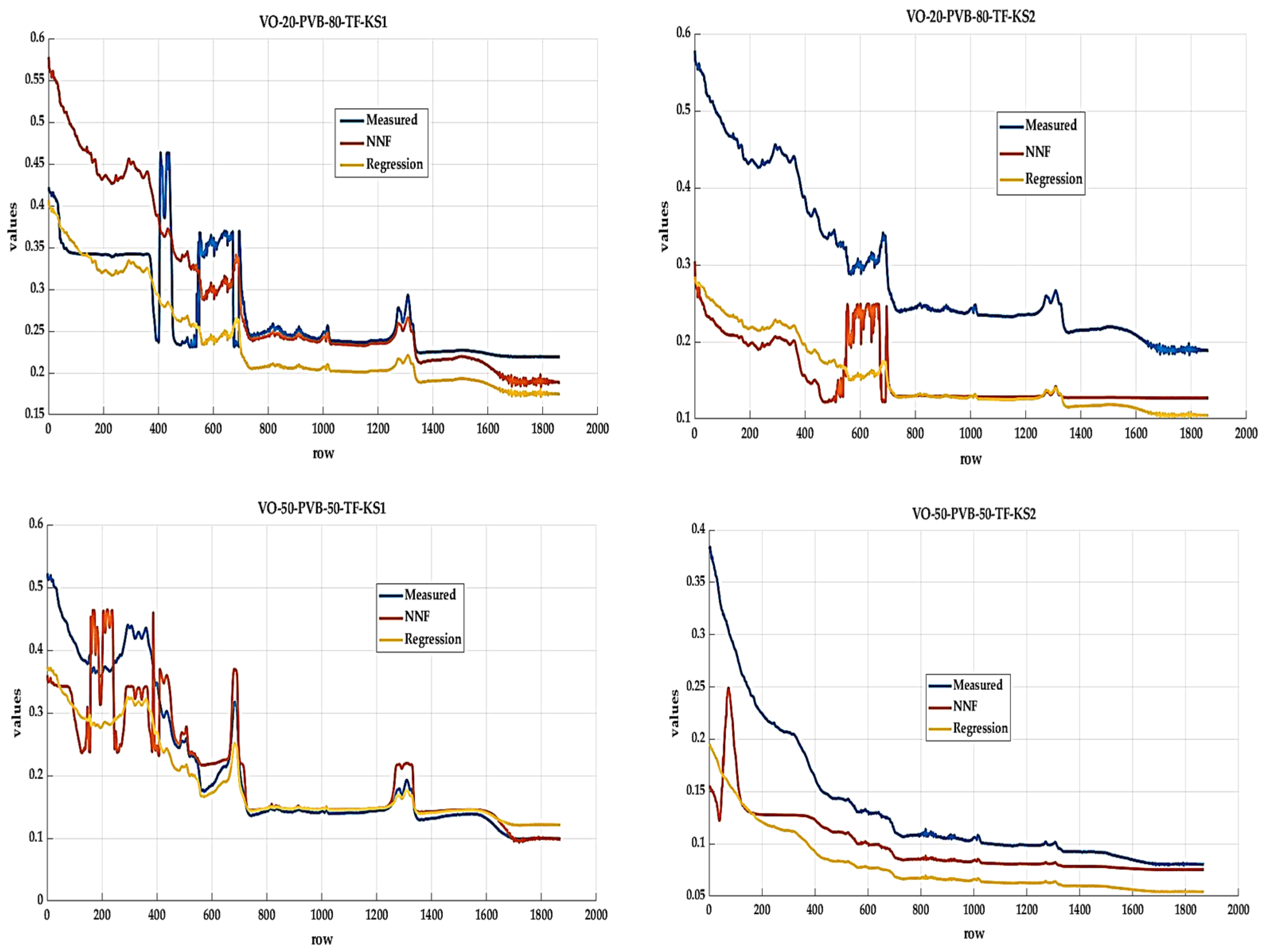
Using both tools, we were allowed to predict new values based on the best models. Since the training set was created by combining values from different materials, it verified (Table 1) its suitability by comparing it with the measured data for individual materials separately.
MS Excel was used to calculate the values. Sample calculation (4) for the first record for material VO_20_PVB_80_TF-KS1.
Based on the results of individual qualitative indicators, it can be seen that the model obtained through neural net fitting achieves better results for both test samples, for both states (KS1 and KS2). This is because the model design environment offers more flexibility to influence individual settings. The “overtraining” option also increases the value of the R coefficient by making the model “learn” more. In the RL environment, it is also possible to influence individual coefficients, but only after generating the function and only by manual change. Variations between test samples may be due to the fact that the created models were only applied to the actual sample size—that is, to 1869 values.
Available data (Figure 9) pairing, validation, and selection procedures are involved in implementing the prediction management model.
The model designed using the neural net fitting tool achieves better results of qualitative indicators. We will apply this model to obtain the assumed values for the material VO_30_PVB_70_TF.
Application of Selected Model for VO_30_PVB_70_TF
This material was not subjected to tests and measurements in a climatic chamber. We will use the selected model to predict these values. From the original set of values, the essential column will be “Absorbance”, which forms the basic input for both models. The following Table 2 shows some of the source values.
By importing the values into the Matlab environment and subsequent modification, we will use the generated functions of the selected model and get the expected KS1 and KS2 values for the assessed material (Figure 10).
The next figure shows a graphical interpretation of gained data using the selected model. The values of “Absorbance” are measured and values of “KS1” and”KS2” are predicted.
The next Table 3 shows part of the gained values KS1 and KS2 for the observed material.
Experiments in the climate chamber require careful planning, take a certain amount of time, and are also financially demanding. The goal of this paper was to predict the absorption values for the material VO_30_70_PVB_TF, which was not subjected to the test in the climate chamber. The authors consider the creation of a model to be a benefit, which will enable obtaining values of the impact of possible climate changes on a material with a given structure, which was not tested in a climate chamber. By using the Matlab tool, we can obtain both the graphical form and numerical values of the observed property.
In the research mentioned above, a model was selected using the Matlab environment tools, which can estimate possible values for the selected materials. The basis of the model is real measured data, which can be expanded, and other data, which opens the way for further improvement of the model. If real measurements are also carried out for the given material, it is possible to compare the measured and acquired data, and thus verify the selected model. The economic benefit of the research is that testing in climate chambers is relatively financially demanding and is almost always a matter for external companies. Delivering the given samples and then taking over the measured data is necessary. There is a risk, albeit minimal, that there may be an error in data transmission, or some data may be lost. The resulting model was created with absorption values with a different percentage distribution of individual components. The suitability was verified through the available data of individual samples. It can also be used for other materials containing the same components in a different percentage representation or used for the other types of thermoplastic materials.
5. Conclusions
The use of composite materials is increasing every year. It is assumed that this trend will continue in the coming years. Currently, the low weight of these materials, their durability, formability, and easy maintenance are especially appreciated. However, the methods by which it would be possible to determine the individual characteristics of these materials more precisely remain a problem. Testing materials obtained the data used in a climate chamber, namely seven cycles, which took 70 h (marked as KS1 in the post) and 32 cycles—which took 320 h (marked as KS2 in the post). In the case of creating new material with the same components, it is possible to use the proposed model. Thus, the results with a given probability are available for assessment in a very short time. In the case of improvement of the model, since the model was created in the Matlab programming environment and the relevant functions are generated, the given model can subsequently be modified using new data sets. It is in this field that the primary concern is the development of predictive models for one or more variables of interest using relevant independent variables or inputs. One of the effective methods is the use of machine learning (ML). ML models are more efficient in the design phase because they allow you to manage massive and large data sets to get the most appropriate or predictive application [24,37]. In the submitted article, effective tools of the Matlab software were pointed out, which enable the design of a model using several artificial intelligence techniques. A model was created that simulated absorption values after testing samples in a climate chamber. Based on the developed model, absorption values were predicted for the material VO_30_70_PVB_TF, which was not tested. Further research will focus on using individual elements of Industry 5.0, specifically for helping artificial intelligence in collecting and predicting errors in the analysis of individual samples.
Author Contributions
Conceptualization, L.K.; methodology, L.K. and S.H.; software, S.H.; validation, S.H.; formal analysis L.K.; investigation, S.H. and L.K. resources, L.K.; data curation, S.H., writing—original draft preparation, L.K.; writing—review and editing, S.H.; visualization, S.H.; funding, L.K.; supervision, L.K. and S.H. All authors have read and agreed to the published version of the manuscript.
Funding
VEGA 1/0268/22 “Design of a Digital Twin for Monitoring the Production Parameters of Technological Equipment Using Augmented Reality”.
Institutional Review Board Statement
Not applicable.
Informed Consent Statement
Not applicable.
Data Availability Statement
Not applicable.
Conflicts of Interest
The authors declare no conflict of interest.
References
- Chen, C.T.; Gu, G.X. Machine learning for composite materials. MRS Commun. 2019, 9, 556. [Google Scholar] [CrossRef] [Green Version]
- Breque, M.; de Nul, L.; Petridis, A. Industry 5.0, Towards a Sustainable, Human-Centric and Resilient European Industry; European Commission: Brussels, Belgium, 2021. [Google Scholar]
- Industry 5.0. Available online: https://research-and-innovation.ec.europa.eu/research-area/industry/industry-50_en (accessed on 15 September 2022).
- Rodríguez-Martín, M.; Fueyo, J.G.; Gonzalez-Aguilera, D.; Madruga, F.J.; García-Martín, R.; Muñóz, Á.L.; Pisonero, J. Predictive Models for the Characterization of Internal Defects in Additive Materials from Active Thermography Sequences Supported by Machine Learning Methods. Sensors 2020, 20, 3982. [Google Scholar] [CrossRef]
- Furtado, C.; Pereira, L.F.; Tavares, R.P.; Salgado, M.; Otero, F.; Catalanotti, G.; Arteiro, A.; Bessa, M.A.; Camanho, P.P. A methodology to generate design allowables of composite laminates using machine learning. Int. J. Solids Struct. 2021, 233, 111095. [Google Scholar] [CrossRef]
- Sharma, A.; Mukhopadhyay, T.; Rangappa, S.M.; Siengchin, S.; Kushvaha, V. Advances in Computational Intelligence of Polymer Composite Materials: Machine Learning Assisted Modeling, Analysis and Design. Arch. Comput. Methods Eng. 2022, 29, 3341–3385. [Google Scholar] [CrossRef]
- Hrehova, S. Quality Evaluation of Heating Process Control Using Matlab Tools. In Proceedings of the 19th International Carpathian Control Conference (ICCC), IEEE, Szilvasvarad, Hungary, 28–31 May 2018. [Google Scholar] [CrossRef]
- Mathworks. Machine Learning. Available online: https://www.mathworks.com/help/stats/machine-learning-in-matlab.html (accessed on 13 March 2022).
- Artificial Neural Networks Overview. Available online: https://www.dataversity.net/artificial-neural-networks-overview/# (accessed on 11 March 2022).
- Paluszek, M.; Thomas, S. Practical MATLAB Deep Learning; Apress: Berkeley, CA, USA, 2020; p. 270. [Google Scholar]
- Hošovský, A.; Piteľ, J.; Trojanová, M.; Židek, K. Computational Intelligence in the Context of Industry 4.0. Implementing Industry 4.0 in SMEs; Palgrave Macmillan: Cham, Switzerland, 2021. [Google Scholar] [CrossRef]
- Bhattacharya, S.; Kalita, K.; Čep, R.; Chakraborty, S. A Comparative Analysis on Prediction Performance of Regression Models during Machining of Composite Materials. Materials 2021, 14, 6689. [Google Scholar] [CrossRef] [PubMed]
- Sinay, J.; Kotianova, Z.; Balazikova, M.; Dulebová, M.; Markulik, Š. Measurement of low-frequency noise during CNC machining and its assessment. Measurement 2018, 119, 190–195. [Google Scholar] [CrossRef]
- Emmert-Streib, F.; Dehmer, M. Evaluation of Regression Models: Model Assessment, Model Selection and Generalization Error. Mach. Learn. Knowl. Extr. 2019, 1, 521–551. [Google Scholar] [CrossRef] [Green Version]
- Inyurt, S.; Kashani, M.H.; Sekertekin, A. Ionospheric TEC forecasting using Gaussian Process Regression (GPR) and Multiple Linear Regression (MLR) in Turkey. Astrophys. Space Sci. 2020, 365, 99. [Google Scholar] [CrossRef]
- Nagyova, A.; Pacaiova, H.; Markulik, S.; Turisová, R.; Kozel, R.; Džugan, J. Design of a Model for Risk Reduction in Project Management in Small and Medium-Sized Enterprises. Symetry 2021, 13, 763. [Google Scholar] [CrossRef]
- Priya, K.S. Linear Regression Algorithm in Machine Learning through MATLAB. Int. J. Res. Appl. Sci. Eng. Technol. (IJRASET) 2021, 9, 12. [Google Scholar] [CrossRef]
- Hamidi, Y.K.; Berrado, A.; Altan, M.C. Machine learning applications in polymer composites. AIP Conf. Proc. 2020, 2205, 20031. [Google Scholar] [CrossRef]
- Anuar, M.A.R.B.K.; Ngamkhanong, C.; Wu, Y.; Kaewunruen, S. Recycled Aggregates Concrete Compressive Strength Prediction Using Artificial Neural Networks (ANNs). Infrastructures 2021, 6, 17. [Google Scholar] [CrossRef]
- Cvitic’, I.; Perakovic’, D.; Perisa, M.; Gupta, B.B. Ensemble machine learning approach for classification of IoT devices in smart home. Int. J. Mach. Learn. Cybern. Ensemble 2021, 12, 3179–3202. [Google Scholar] [CrossRef]
- Jierula, A.; Wang, S.; Oh, T.-M.; Wang, P. Study on Accuracy Metrics for Evaluating the Predictions of Damage Locations in Deep Piles Using Artificial Neural Networks with Acoustic Emission Data. Appl. Sci. 2021, 11, 2314. [Google Scholar] [CrossRef]
- Straka, M.; Rosová, A.; Radim, L.; Petr, B.; Janka, Š. Principles of computer simulation design for the needs of improvement of the raw materials combined transport system. Acta Montan. Slovaca 2018, 23, 163–174. [Google Scholar]
- Malindzakova, M.; Straka, M.; Rosova, A.; Kanuchova, M.; Trebuna, P. Modeling the process for incineration of municipal waste. Przem. Chem. 2015, 94, 1260–1264. [Google Scholar] [CrossRef]
- Wicher, P.; Staš, D.; Karkula, M.; Lenort, R.; Besta, P. A computer simulation-based analysis of supply chains resilience in industrial environment. Metalurgija 2015, 54, 703–706. [Google Scholar]
- Szavai, S.; Kovacs, S.; Bezi, Z.; Kozak, D. Coupled Numerical Method for Rolling Contact Fatigue Analysis. Teh. Vjesn. Tech. Gaz. 2021, 28, 1560–1567. [Google Scholar] [CrossRef]
- Gupta, B.B.; Tewari, A.; Cvitic, I.; Perakovic, D.; Chang, X.J. Articial intelligence empowered emals classifier for Internet of Things based system in industry 4.0. Wirel. Netw. 2022, 28, 493–503. [Google Scholar] [CrossRef]
- Cvitic´, I.; Perakovic´, D.; Periša, M.; Botica, M. Novel approach for detection of IoT generated DDoS traffic. Wirel. Netw. 2019, 27, 1573–1586. [Google Scholar] [CrossRef]
- Gubbi, J.; Buyya, R.; Marusic, S.; Palaniswami, M. Internet of Things (IoT): A vision, architectural elements, and future directions. Future Gener. Comput. Syst. 2013, 29, 1645–1660. [Google Scholar] [CrossRef] [Green Version]
- Atzori, L.; Iera, A.; Morabito, G. The Internet of Things: A survey. Comput. Netw. 2010, 54, 2787–2805. [Google Scholar] [CrossRef]
- Georgala, K.; Kosmopoulos, A.; Paliouras, G. Spam filtering: An active learning approach using incremental clustering. In Proceedings of the 4th International Conference on Web Intelligence, Mining and Semantics, Thessaloniki, Greece, 2–4 June 2014. [Google Scholar]
- Xie, Z.; Peng, J.; Sorokina, M.; Zeng, H. Design of Mode-Locked Fibre Laser with Non-Linear Power and Spectrum Width Transfer Functions with a Power Threshold. Appl. Sci. 2022, 12, 10318. [Google Scholar] [CrossRef]
- Behunova, A.; Soltysova, Z.; Behun, M. Complexity Management and its impact on economy. TEM J. Technol. Educ. Manag. Inform. 2018, 7, 324–329. [Google Scholar] [CrossRef]
- Grabara, J.K.; Dima, I.C.; Kot, S.; Kwiatkowska, J. Case on in-house logistics modeling and simulation. Res. J. Appl. Sci. 2011, 6, 7–12. [Google Scholar] [CrossRef] [Green Version]
- Gor, M.; Dobriyal, A.; Wankhede, V.; Sahlot, P.; Grzelak, K.; Kluczyński, J.; Łuszczek, J. Density Prediction in Powder Bed Fusion Additive Manufacturing: Machine Learning-Based Techniques. Appl. Sci. 2022, 12, 7271. [Google Scholar] [CrossRef]
- Kot, S.; Slusarczyk, B. Process simulation in supply chain using logware software. Ann. Univ. Apulensis Ser. Oeconomica 2009, 11, 932. [Google Scholar]
- Schmid, J.; Trabesinger, S.; Brillinger, M.; Pichler, R.; Wurzinger, J.; Ciumasu, R. Tacit Knowledge Based Acquisition of Verified Machining Data. In Proceedings of the IEEE, 9th International Conference on Industrial Technology and Management (ICITM 2020), Oxford, UK, 11–13 February 2020; pp. 117–121. [Google Scholar]
- Yu, J.; Oh, S.J.; Baek, S.; Kim, J.; Lee, T. Predicting the Effect of Processing Parameters on Caliber-Rolled Mg Alloys through Machine Learning. Appl. Sci. 2022, 12, 10646. [Google Scholar] [CrossRef]
Figure 1.
Three pillars of Industry 5.0 [2].
Figure 1.
Three pillars of Industry 5.0 [2].

Figure 2.
The main components for composites [authors’ own processing].

Figure 3.
Results for VO_20_PVB_80_TF [authors’ own processing].

Figure 4.
Results for VO_50_PVB_50_TF [authors’ own processing].

Figure 5.
Machine learning dividing [10].
Figure 5.
Machine learning dividing [10].

Figure 6.
Scheme of the fitting neural network [authors’ own processing].

Figure 7.
Plot regression results [authors’ own processing].

Figure 8.
Regression learner environment—a prediction model [authors own processing].

Figure 9.
Graphic representation of the proposed models [authors own processing].

Figure 10.
Graphic representation of the predicted values of KS1 and KS2 [authors’ own processing].


Table 1.
Comparison of proposed models [authors’ own processing].
| Method | Neural Net Fitting | Regression Learner | ||||||
|---|---|---|---|---|---|---|---|---|
| Material | VO-20-PVB-80-TF | VO-50-PVB-50-TF | VO-20-PVB-80-TF | VO-50-PVB-50-TF | ||||
| State | KS1 | KS2 | KS1 | KS2 | KS1 | KS2 | KS1 | KS2 |
| R2 | 0.9052 | 0.9866 | 0.7302 | 0.8655 | 0.7617 | 0.6325 | 0.6448 | 0.5659 |
| MAPE | 8.56% | 11.21% | 12.04% | 15.37% | 14.92% | 27.11% | 18.64% | 29.45% |
| MSE | 0.00094 | 0.000708 | 0.00359 | 0.00209 | 0.00237 | 0.00432 | 0.00473 | 0.00188 |
Table 2.
Some of the source values by the sample absorbance.
| Values | ||||||||
|---|---|---|---|---|---|---|---|---|
| Wave | 399.19 | 401.12 | 403.05 | 404.97 | 406.90 | 408.83 | 410.76 | 412.69 |
| Absorbance | 0.774 | 0.778 | 0.777 | 0.769 | 0.762 | 0.757 | 0.762 | 0.772 |
Table 3.
Predicted values of KS1 and KS2 for VO_30_70_PVB_TF [authors own processing].
| Values | ||||||||
|---|---|---|---|---|---|---|---|---|
| Absorbance | 0.774 | 0.778 | 0.777 | 0.769 | 0.762 | 0.757 | 0.762 | 0.772 |
| KS1 | 0.5702 | 0.5707 | 0.5705 | 0.5692 | 0.5676 | 0.5659 | 0.5675 | 0.5697 |
| KS2 | 0.6809 | 0.6865 | 0.6850 | 0.6702 | 0.6495 | 0.6288 | 0.6482 | 0.6759 |
Publisher’s Note: MDPI stays neutral with regard to jurisdictional claims in published maps and institutional affiliations. |
© 2022 by the authors. Licensee MDPI, Basel, Switzerland. This article is an open access article distributed under the terms and conditions of the Creative Commons Attribution (CC BY) license (https://creativecommons.org/licenses/by/4.0/).
Share and Cite
MDPI and ACS Style
Hrehova, S.; Knapcikova, L. The Study of Machine Learning Assisted the Design of Selected Composites Properties. Appl. Sci. 2022, 12, 10863. https://0-doi-org.brum.beds.ac.uk/10.3390/app122110863
AMA Style
Hrehova S, Knapcikova L. The Study of Machine Learning Assisted the Design of Selected Composites Properties. Applied Sciences. 2022; 12(21):10863. https://0-doi-org.brum.beds.ac.uk/10.3390/app122110863
Chicago/Turabian StyleHrehova, Stella, and Lucia Knapcikova. 2022. "The Study of Machine Learning Assisted the Design of Selected Composites Properties" Applied Sciences 12, no. 21: 10863. https://0-doi-org.brum.beds.ac.uk/10.3390/app122110863
Note that from the first issue of 2016, this journal uses article numbers instead of page numbers. See further details here.