Author Contributions
Conceptualization, J.V.-O., A.T.-C., D.I.-G. and N.M.; Data curation, A.T.-C. and C.P.-d.-l.-L.; Formal Analysis, J.V.-O. and A.T.-C.; Funding acquisition, A.T.-C., Y.R. and N.M.; Investigation, J.V.-O., A.T.-C. and C.P.-d.-l.-L.; Methodology, J.V.-O., A.T.-C., C.P.-d.-l.-L., D.I.-G. and N.M.; Resources, A.T.-C., O.A.C., Y.R., F.M., A.S., M.S., D.I.-G. and N.M.; Software, J.V.-O. and A.T.-C.; Supervision, A.T.-C., D.I.-G. and N.M.; Validation, J.V.-O., A.T.-C. and C.P.-d.-l.-L.; Visualization, J.V.-O., A.T.-C. and C.P.-d.-l.-L., Writing—original draft preparation, J.V.-O. and A.T.-C., C.P.-d.-l.-L., D.I.-G. and N.M.; writing—review and editing, J.V.-O., A.T.-C., C.P.-d.-l.-L., O.A.C., Y.R., F.M., A.S., M.S., D.I.-G. and N.M. All authors have read and agreed to the published version of the manuscript.
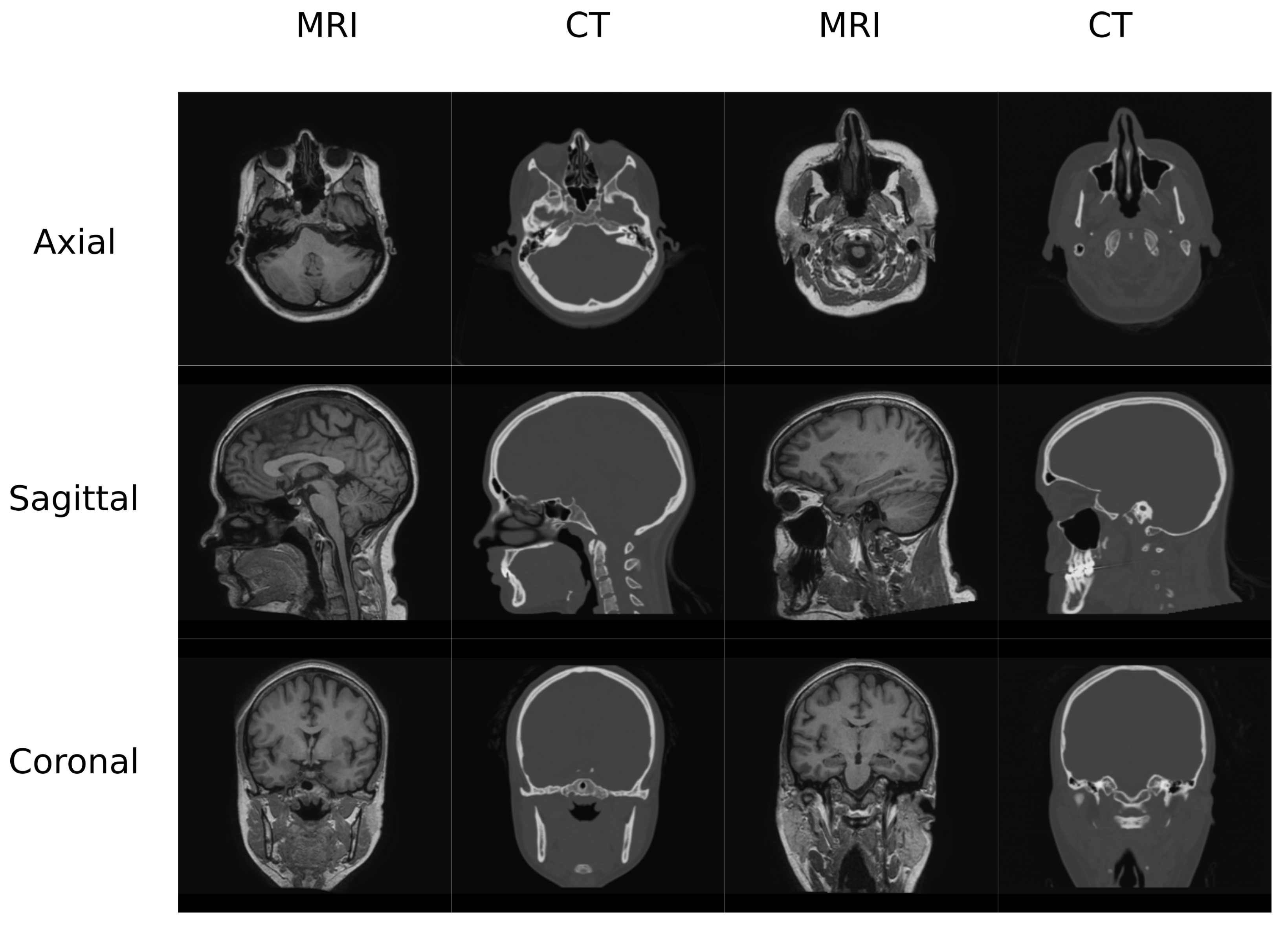
Figure 1.
Head Data set example.
Figure 1.
Head Data set example.
Figure 2.
Pelvis Data set example.
Figure 2.
Pelvis Data set example.
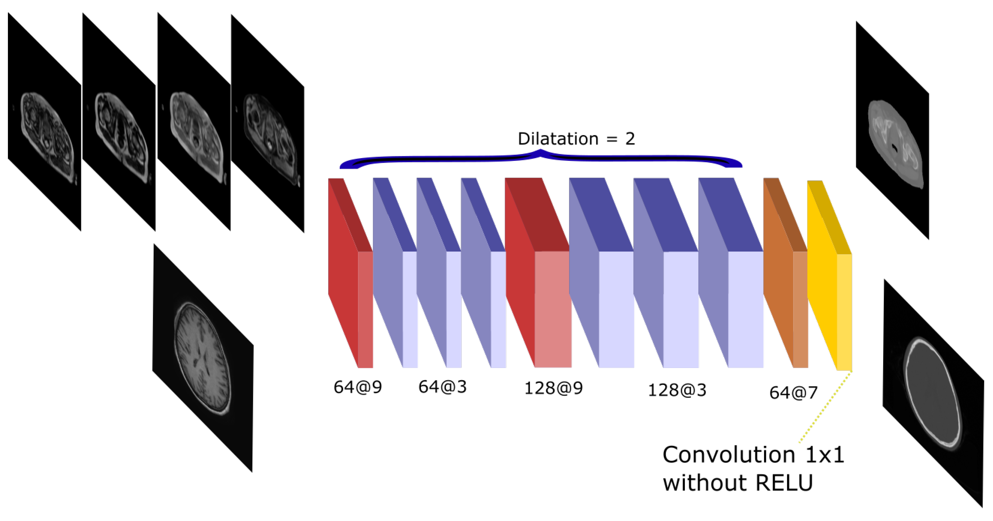
Figure 3.
Atrous-Net architecture. The scheme shows the CNN architecture including the atrous convolutions. The network receives either the four Dixon-VIBE MR sequences of the pelvis or the T1-weighted image of the brain as input. Then, it outputs a pelvis or a head pseudo-CT, respectively.
Figure 3.
Atrous-Net architecture. The scheme shows the CNN architecture including the atrous convolutions. The network receives either the four Dixon-VIBE MR sequences of the pelvis or the T1-weighted image of the brain as input. Then, it outputs a pelvis or a head pseudo-CT, respectively.
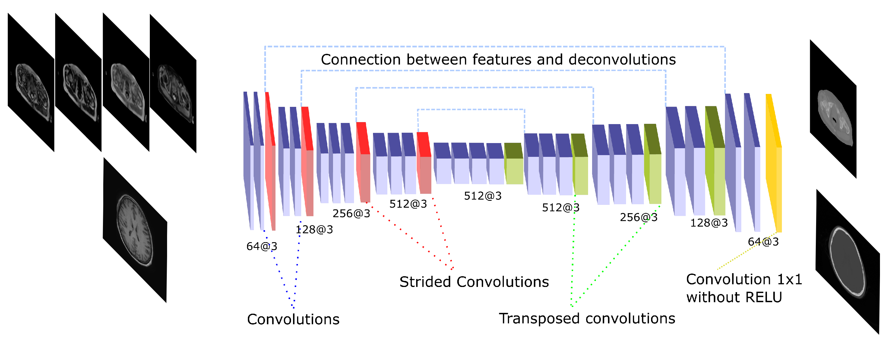
Figure 4.
U-Net architecture. The scheme shows the CNN architecture including the encoder and the decoder blocks that are linked by skip connections. The encoding part presents strided operations while the decoding part is composed by transposed convolutions. The network receives either the four Dixon-VIBE MR sequences of the pelvis or the T1-weighted image of the brain as input. Then, it outputs a pelvis or a head pseudo-CT, respectively.
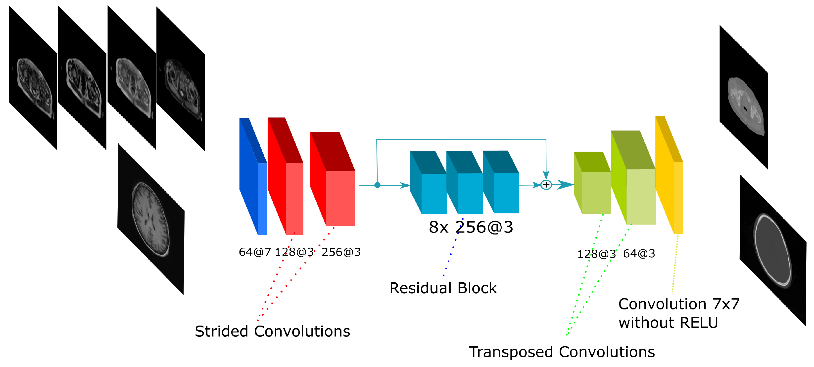
Figure 5.
Residual-Net architecture. The scheme shows the CNN architecture including the residual blocks in between the encoding and the decoding steps. The network receives either the four Dixon-VIBE MR sequences of the pelvis or the T1-weighted image of the brain as input. Then, it outputs a pelvis or a head pseudo-CT, respectively.
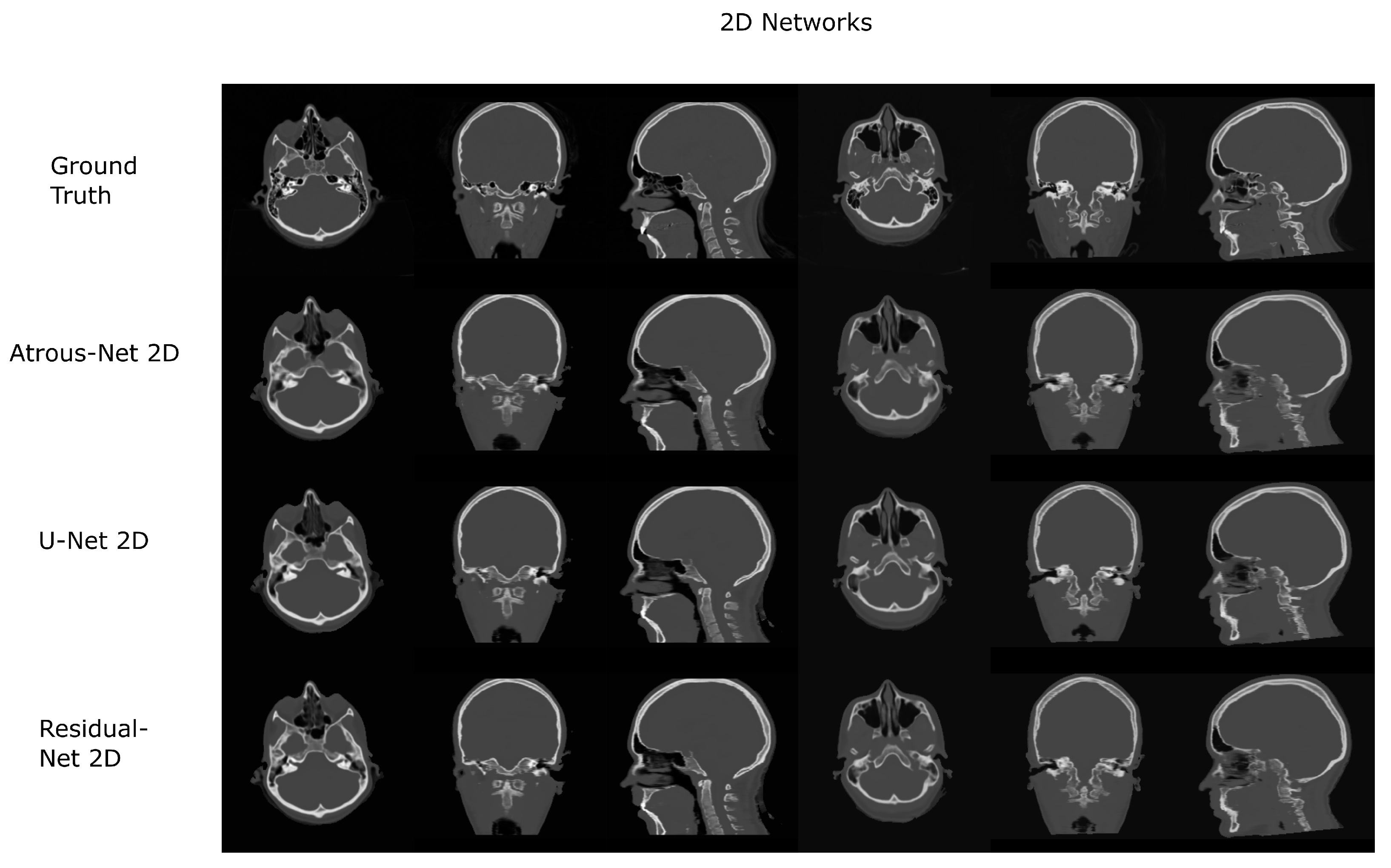
Figure 6.
Head results using 2D networks.
Figure 6.
Head results using 2D networks.
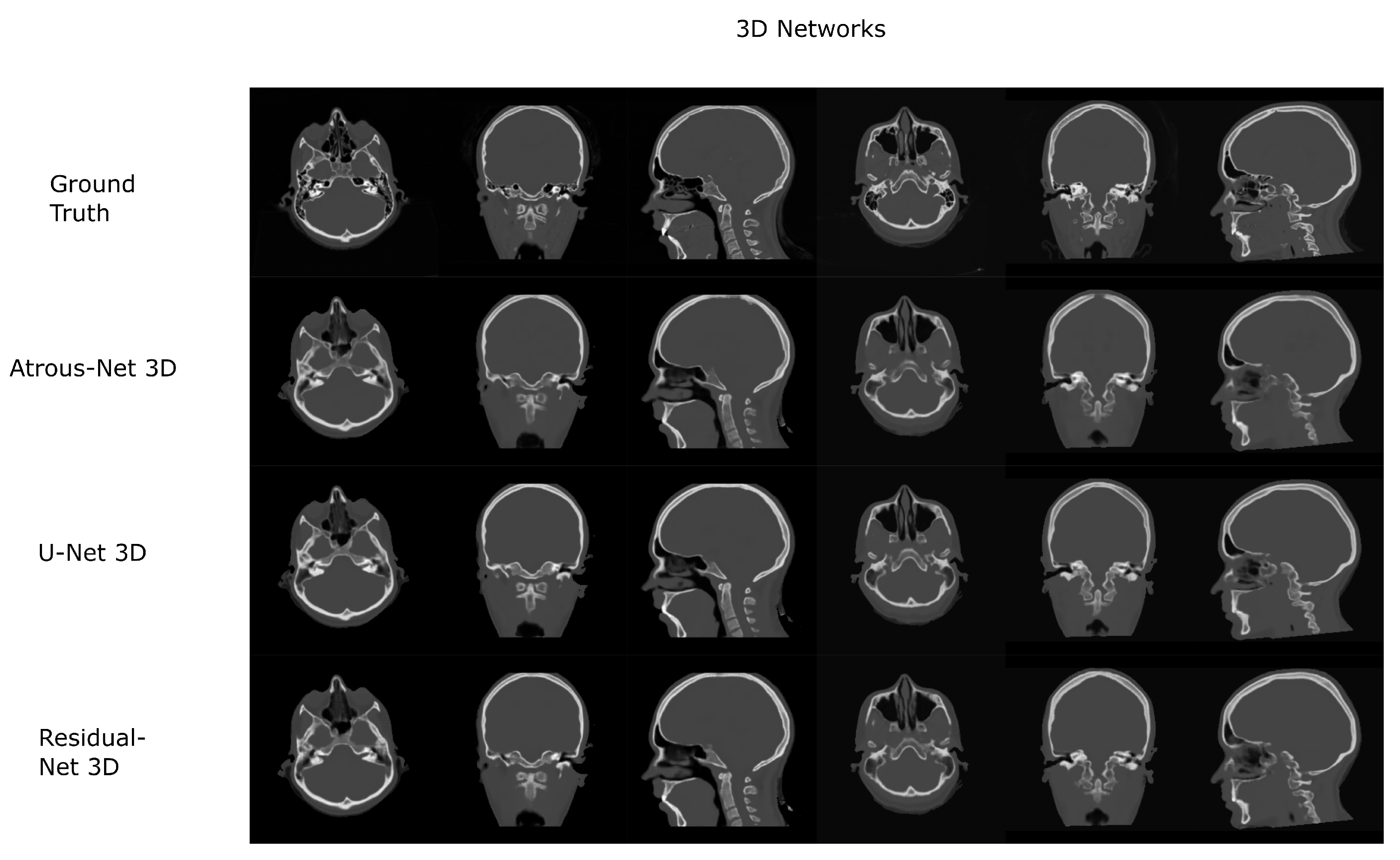
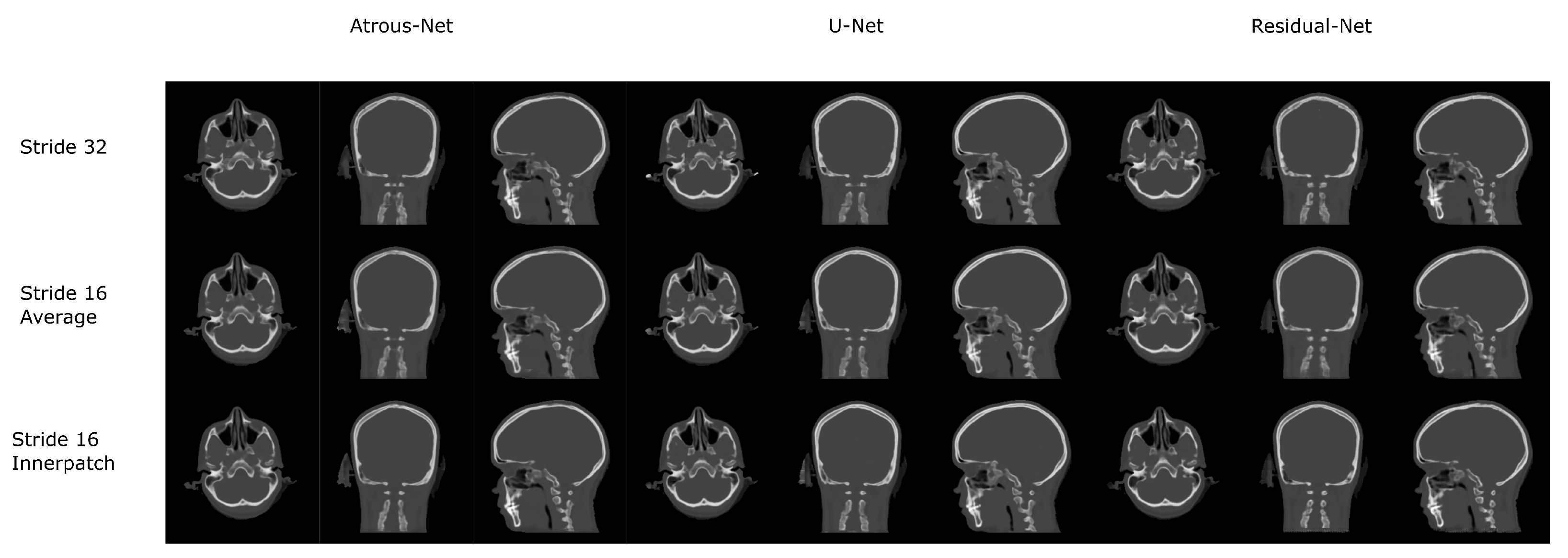
Figure 7.
Head results using 3D-16 networks.
Figure 7.
Head results using 3D-16 networks.
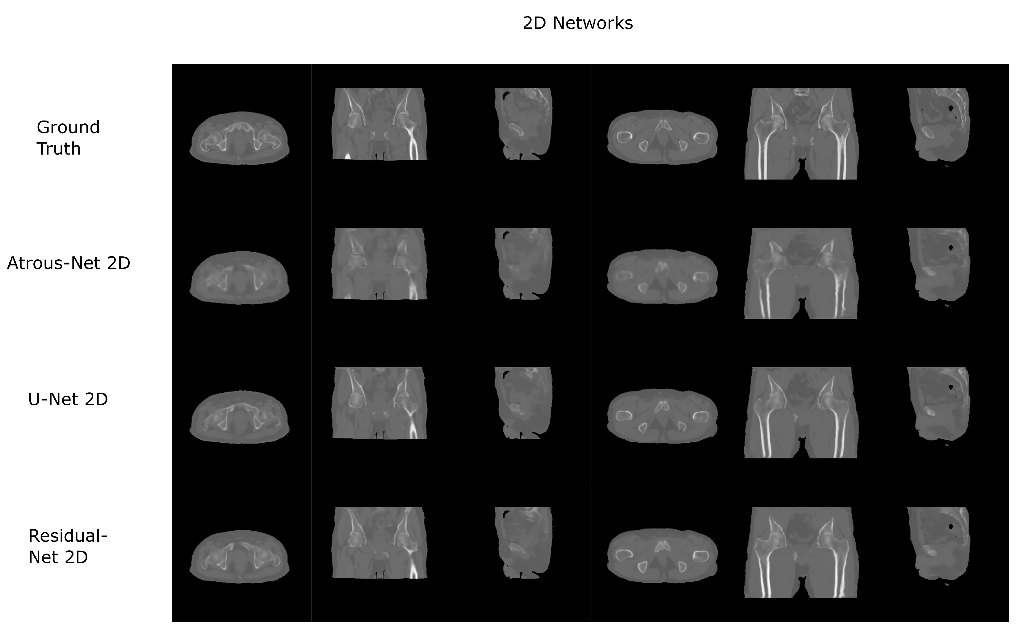
Figure 8.
Pelvis results using 2D networks.
Figure 8.
Pelvis results using 2D networks.
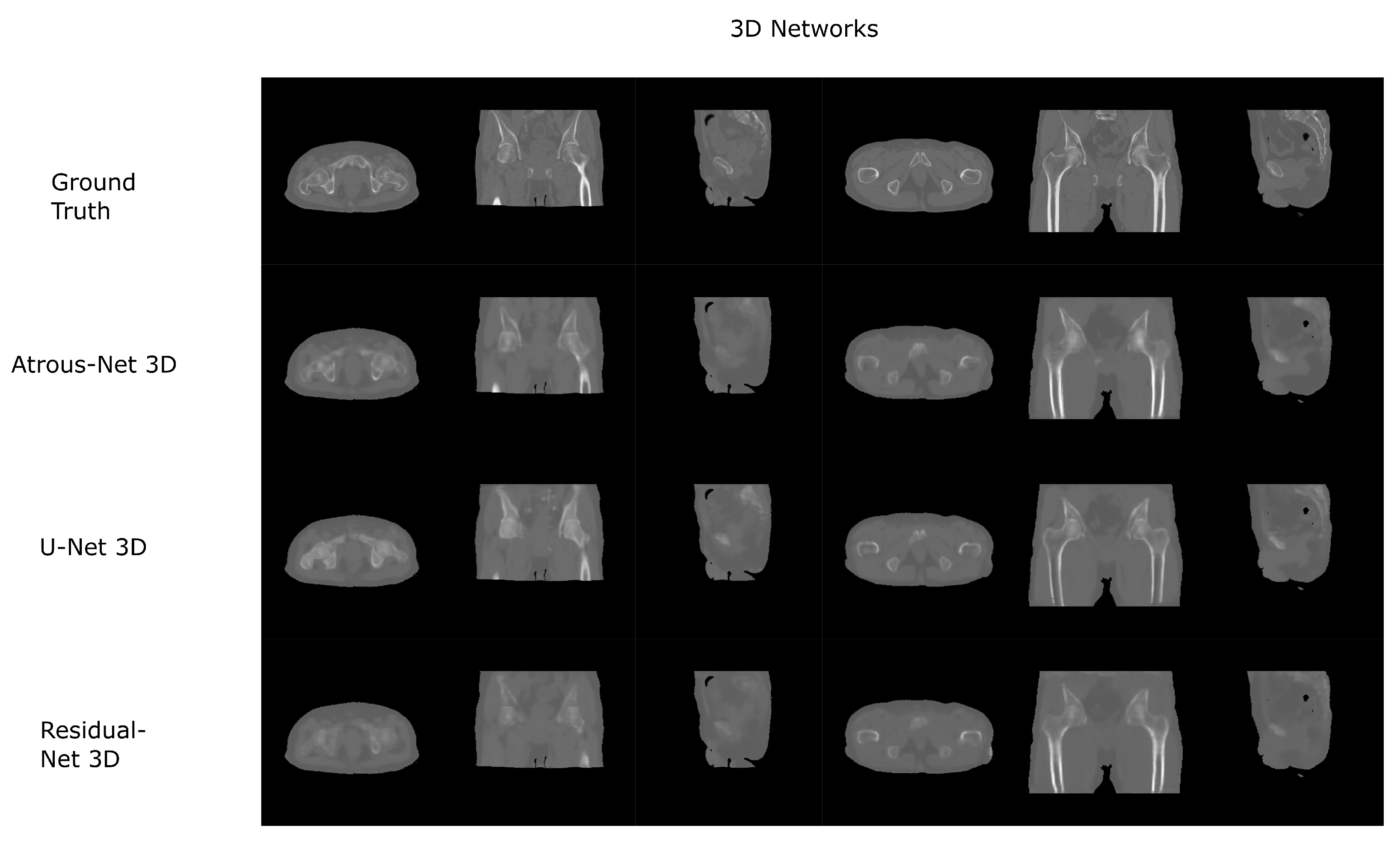
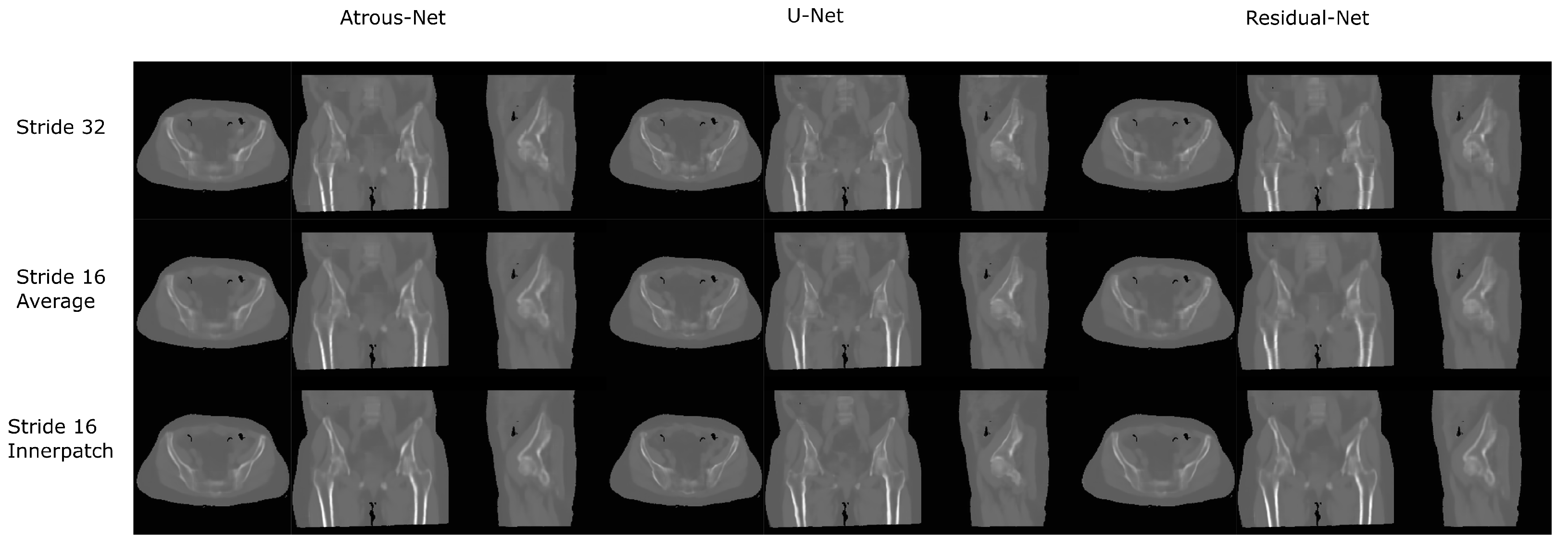
Figure 9.
Pelvis results using 3D-16 networks.
Figure 9.
Pelvis results using 3D-16 networks.
Figure 10.
Comparison between the reconstruction method proposed.
Figure 10.
Comparison between the reconstruction method proposed.
Figure 11.
Comparison between the reconstruction method proposed.
Figure 11.
Comparison between the reconstruction method proposed.
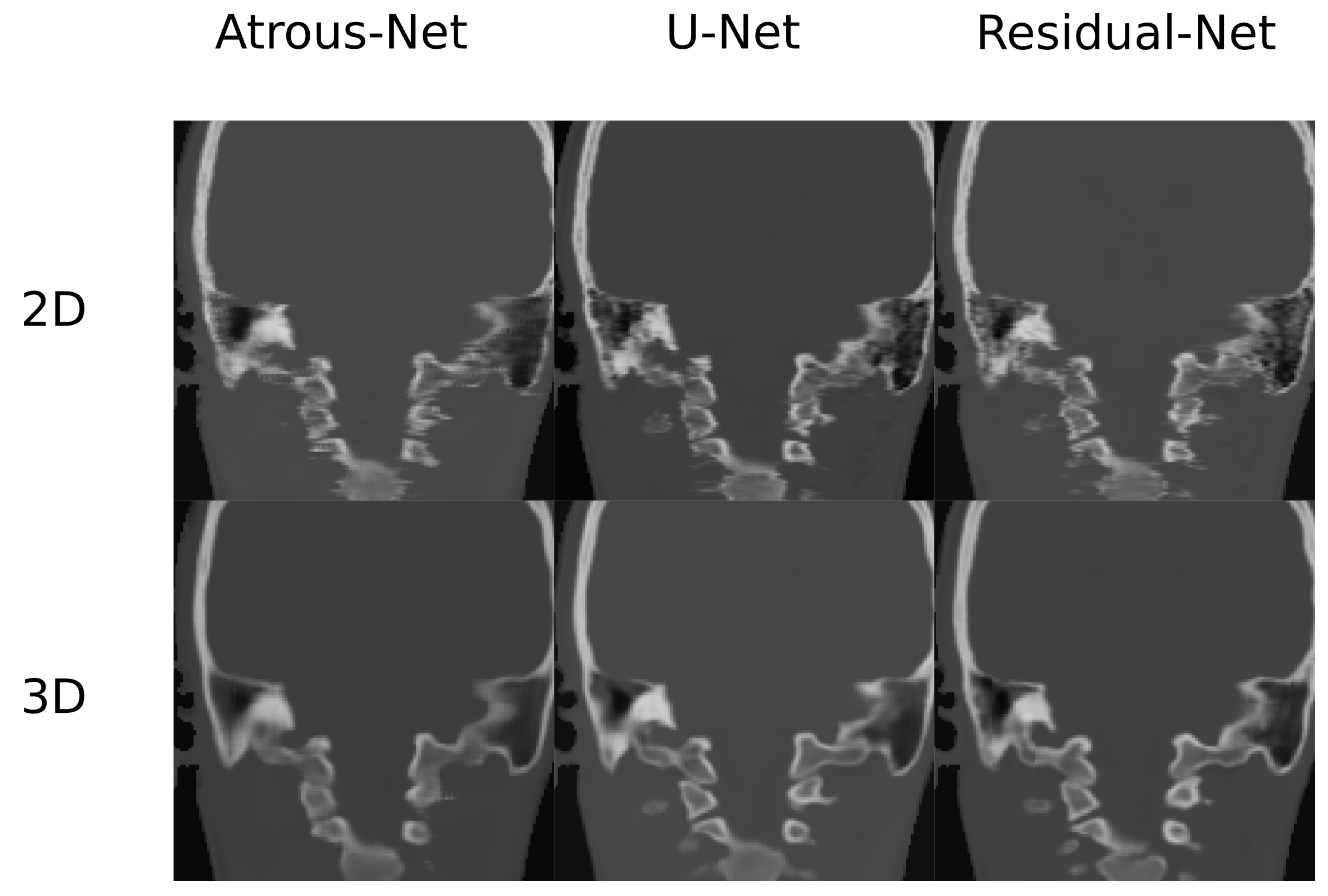
Figure 12.
Comparison in the sagittal and coronal direction for the head between the 2D and 3D schemes.
Figure 12.
Comparison in the sagittal and coronal direction for the head between the 2D and 3D schemes.
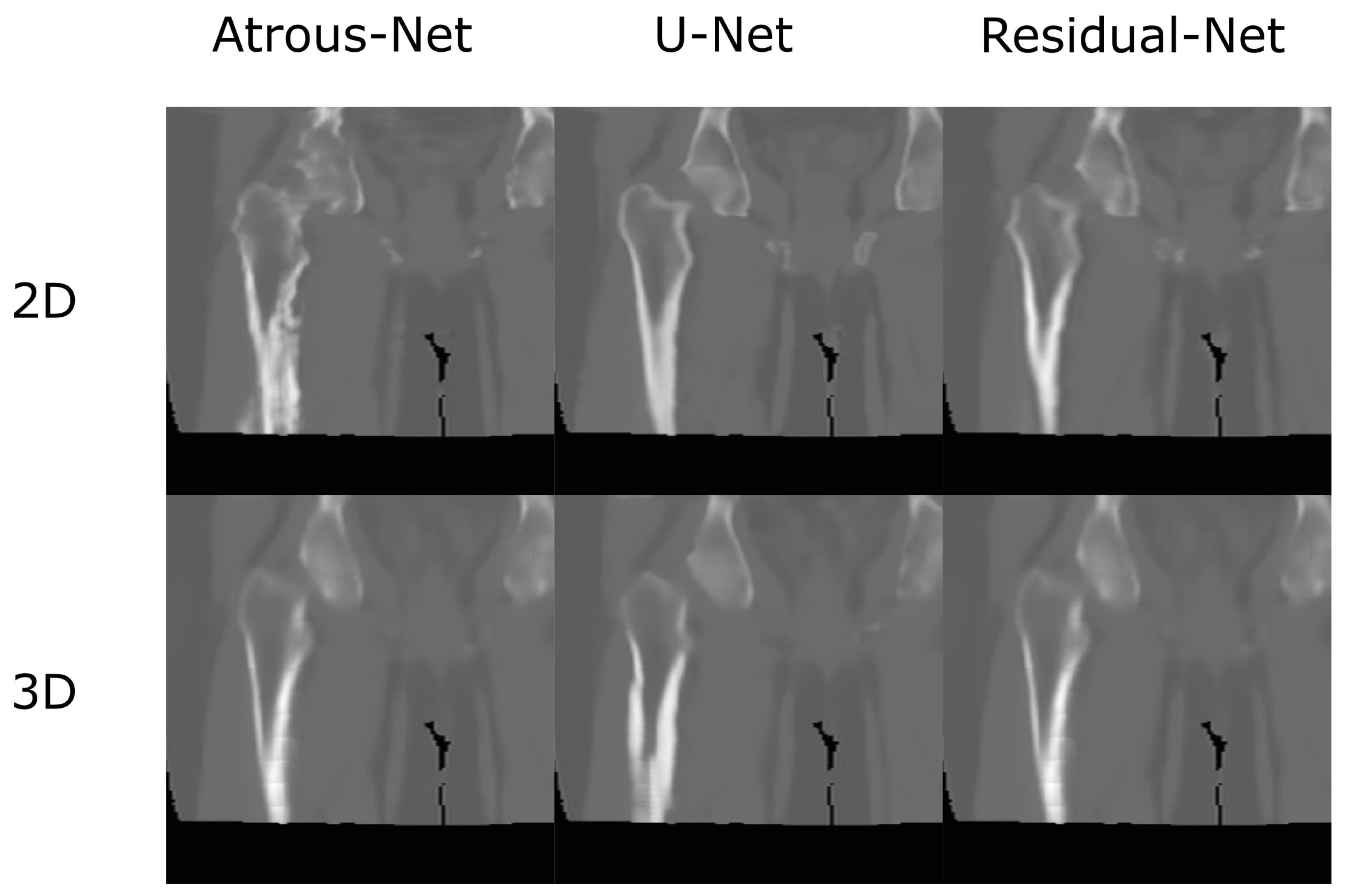
Figure 13.
Comparison in the sagittal and coronal direction for the pelvis between the 2D and 3D schemes.
Figure 13.
Comparison in the sagittal and coronal direction for the pelvis between the 2D and 3D schemes.
Table 1.
Head dataset with U-net. Mean Absolute Error, PSNR and Pearson coefficient on the head data set obtained using U-net with different convolutions and reconstructions.
Table 1.
Head dataset with U-net. Mean Absolute Error, PSNR and Pearson coefficient on the head data set obtained using U-net with different convolutions and reconstructions.
| | MAE | PSNR | Pearson |
|---|
| 2D | 117.21 ± 9.49 | 23.26 ± 0.596 | 0.898 ± 0.011 |
| 3D-32 | 93.45 ± 7.96 | 25.40 ± 0.675 | 0.939 ± 0.010 |
| 3D-16av | 90.06 ± 7.65 | 25.77 ± 0.706 | 0.944 ± 0.010 |
| 3D-16 | 89.54 ± 7.79 | 25.69 ± 0.703 | 0.943 ± 0.009 |
Table 2.
Head dataset with Atrous-Net. Mean Absolute Error, PSNR and Pearson coefficient on the head data set obtained using Atrous network with different convolutions and reconstructions.
Table 2.
Head dataset with Atrous-Net. Mean Absolute Error, PSNR and Pearson coefficient on the head data set obtained using Atrous network with different convolutions and reconstructions.
| | MAE | PSNR | Pearson |
|---|
| 2D | 105.16 ± 8.92 | 24.51 ± 0.615 | 0.924 ± 0.009 |
| 3D-32 | 110.89 ± 7.56 | 24.12 ± 0.546 | 0.917 ± 0.009 |
| 3D-16av | 104.98 ± 7.28 | 25.77 ± 0.706 | 0.926 ± 0.009 |
| 3D-16 | 104.03 ± 6.98 | 24.65 ± 0.555 | 0.927 ± 0.009 |
Table 3.
Head dataset with Residual-Net. Mean Absolute Error, PSNR and Pearson coefficient on the head data set obtained using Residual net with different convolutions and reconstructions.
Table 3.
Head dataset with Residual-Net. Mean Absolute Error, PSNR and Pearson coefficient on the head data set obtained using Residual net with different convolutions and reconstructions.
| | MAE | PSNR | Pearson |
|---|
| 2D | 99.83 ± 8.06 | 24.83 ± 0.613 | 0.931 ± 0.009 |
| 3D-32 | 104.57 ± 8.40 | 24.52 ± 0.681 | 0.925 ± 0.013 |
| 3D-16av | 97.88 ± 7.84 | 25.15 ± 0.626 | 0.935 ± 0.009 |
| 3D-16 | 98.14 ± 7.99 | 24.69 ± 1.280 | 0.927 ± 0.025 |
Table 4.
Head dataset Bone with U-net. Mean Absolute Error, PSNR and Pearson coefficient within the bone on the head data set obtained using U-net with different convolutions and reconstructions.
Table 4.
Head dataset Bone with U-net. Mean Absolute Error, PSNR and Pearson coefficient within the bone on the head data set obtained using U-net with different convolutions and reconstructions.
| | MAE | PSNR | Pearson |
|---|
| 2D | 382.64 ± 23.85 | 17.48 ± 0.577 | 0.757 ± 0.021 |
| 3D-32 | 326.33 ± 15.47 | 19.71 ± 0.362 | 0.849 ± 0.014 |
| 3D-16av | 289.64 ± 15.57 | 20.08 ± 0.382 | 0.860 ± 0.013 |
| 3D-16 | 289.10 ± 15.64 | 20.05 ± 0.384 | 0.861 ± 0.013 |
Table 5.
Head dataset Bone with Atrous-Net. Mean Absolute Error, PSNR and Pearson coefficient within the bone on the head data set obtained using Atrous net with different convolutions and reconstructions.
Table 5.
Head dataset Bone with Atrous-Net. Mean Absolute Error, PSNR and Pearson coefficient within the bone on the head data set obtained using Atrous net with different convolutions and reconstructions.
| | MAE | PSNR | Pearson |
|---|
| 2D | 352.15 ± 19.96 | 18.58 ± 0.441 | 0.811 ± 0.014 |
| 3D-32 | 358.74 ± 15.96 | 18.39 ± 0.385 | 0.798 ± 0.017 |
| 3D-16av | 338.81 ± 17.81 | 18.86 ± 0.410 | 0.816 ± 0.016 |
| 3D-16 | 336.32 ± 15.35 | 18.93 ± 0.359 | 0.821 ± 0.015 |
Table 6.
Head dataset Bone with Residual-Net. Mean Absolute Error, PSNR and Pearson coefficient within the bone on the head data set obtained using Residual net with different convolutions and reconstructions.
Table 6.
Head dataset Bone with Residual-Net. Mean Absolute Error, PSNR and Pearson coefficient within the bone on the head data set obtained using Residual net with different convolutions and reconstructions.
| | MAE | PSNR | Pearson |
|---|
| 2D | 326.33 ± 17.94 | 19.04 ± 0.428 | 0.826 ± 0.012 |
| 3D-32 | 342.42 ± 16.72 | 18.74 ± 0.591 | 0.810 ± 0.023 |
| 3D-16av | 316.70 ± 15.90 | 19.50 ± 0.378 | 0.837 ± 0.013 |
| 3D-16 | 317.12 ± 16.29 | 19.25 ± 0.452 | 0.833 ± 0.015 |
Table 7.
Head dataset Fat with U-net. Mean Absolute Error, PSNR and Pearson coefficient within the fat on the head data set obtained using U-net with different convolutions and reconstructions.
Table 7.
Head dataset Fat with U-net. Mean Absolute Error, PSNR and Pearson coefficient within the fat on the head data set obtained using U-net with different convolutions and reconstructions.
| | MAE | PSNR | Pearson |
|---|
| 2D | 186.28 ± 23.86 | 21.17 ± 1.51 | 0.544 ± 0.075 |
| 3D-32 | 160.85 ± 28.58 | 23.38 ± 1.47 | 0.685 ± 0.079 |
| 3D-16av | 153.23 ± 31.25 | 23.51 ± 1.67 | 0.695 ± 0.083 |
| 3D-16 | 153.31 ± 29.41 | 23.54 ± 1.559 | 0.694 ± 0.079 |
Table 8.
Head dataset Fat with Atrous-Net. Mean Absolute Error, PSNR and Pearson coefficient within the fat on the head data set obtained using Atrous network with different convolutions and reconstructions.
Table 8.
Head dataset Fat with Atrous-Net. Mean Absolute Error, PSNR and Pearson coefficient within the fat on the head data set obtained using Atrous network with different convolutions and reconstructions.
| | MAE | PSNR | Pearson |
|---|
| 2D | 173.62 ± 29.88 | 22.57 ± 1.56 | 0.650 ± 0.079 |
| 3D-32 | 176.96 ± 43.70 | 22.13 ± 1.77 | 0.630 ± 0.087 |
| 3D-16av | 173.45 ± 42.72 | 22.61 ± 1.70 | 0.654 ± 0.080 |
| 3D-16 | 172.99 ± 45.22 | 22.88 ± 1.821 | 0.662 ± 0.083 |
Table 9.
Head dataset Fat with Residual-Net. Mean Absolute Error, PSNR and Pearson coefficient within the fat on the head data set obtained using Residual net with different convolutions and reconstructions.
Table 9.
Head dataset Fat with Residual-Net. Mean Absolute Error, PSNR and Pearson coefficient within the fat on the head data set obtained using Residual net with different convolutions and reconstructions.
| | MAE | PSNR | Pearson |
|---|
| 2D | 157.11 ± 24.30 | 22.85 ± 1.59 | 0.662 ± 0.078 |
| 3D-32 | 168.65 ± 24.25 | 22.35 ± 1.432 | 0.646 ± 0.072 |
| 3D-16av | 158.88 ± 25.08 | 22.94 ± 1.539 | 0.666 ± 0.075 |
| 3D-16 | 159.20 ± 24.66 | 22.72 ± 1.404 | 0.659 ± 0.069 |
Table 10.
Head dataset Soft-tissue with U-net. Mean Absolute Error, PSNR and Pearson coefficient within the soft-tissue on the head data set obtained using U-net with different convolutions and reconstructions.
Table 10.
Head dataset Soft-tissue with U-net. Mean Absolute Error, PSNR and Pearson coefficient within the soft-tissue on the head data set obtained using U-net with different convolutions and reconstructions.
| | MAE | PSNR | Pearson |
|---|
| 2D | 29.43 ± 4.08 | 33.66 ± 1.70 | 0.326 ± 0.046 |
| 3D-32 | 23.78 ± 3.47 | 35.16 ± 1.288 | 0.346 ± 0.050 |
| 3D-16av | 22.21 ± 3.70 | 35.58 ± 1.144 | 0.337 ± 0.040 |
| 3D-16 | 22.67 ± 3.24 | 35.12 ± 1.143 | 0.342 ± 0.044 |
Table 11.
Head dataset Soft-tissue with Atrous-Net. Mean Absolute Error, PSNR and Pearson coefficient within the soft-tissue on the head data set obtained using Atrous net with different convolutions and reconstructions.
Table 11.
Head dataset Soft-tissue with Atrous-Net. Mean Absolute Error, PSNR and Pearson coefficient within the soft-tissue on the head data set obtained using Atrous net with different convolutions and reconstructions.
| | MAE | PSNR | Pearson |
|---|
| 2D | 27.94 ± 3.98 | 33.75 ± 1.124 | 0.329 ± 0.045 |
| 3D-32 | 30.36 ± 4.07 | 33.10 ± 1.482 | 0.296 ± 0.074 |
| 3D-16av | 27.96 ± 3.79 | 33.04 ± 1.407 | 0.334 ± 0.078 |
| 3D-16 | 27.79 ± 4.08 | 32.66 ± 1.708 | 0.332 ± 0.090 |
Table 12.
Head dataset Soft-tissue with Residual-Net. Mean Absolute Error, PSNR and Pearson coefficient within the bone on the head data set obtained using Residual net with different convolutions and reconstructions.
Table 12.
Head dataset Soft-tissue with Residual-Net. Mean Absolute Error, PSNR and Pearson coefficient within the bone on the head data set obtained using Residual net with different convolutions and reconstructions.
| | MAE | PSNR | Pearson |
|---|
| 2D | 27.18 ± 3.47 | 33.65 ± 1.093 | 0.338 ± 0.047 |
| 3D-32 | 29.19 ± 4.72 | 33.30 ± 1.148 | 0.328 ± 0.037 |
| 3D-16av | 27.61 ± 4.41 | 33.86 ± 1.21 | 0.350 ± 0.042 |
| 3D-16 | 27.69 ± 3.69 | 33.38 ± 1.063 | 0.341 ± 0.040 |
Table 13.
MAE and PSNR p-values for 2D Head. p-values of paired Student’s t-test for MAE and PSNR results with 2D architectures with the head dataset.
Table 13.
MAE and PSNR p-values for 2D Head. p-values of paired Student’s t-test for MAE and PSNR results with 2D architectures with the head dataset.
| PSNR\MAE | Residual-Net | Atrous-Net | U-Net |
|---|
| Residual-Net | - | | |
| Atrous-Net | | - | |
| U-Net | | | - |
Table 14.
MAE and PSNR p-values for 3D Head. p-values of paired Student’s t-test for MAE and PSNR results with 3D architectures with the head dataset.
Table 14.
MAE and PSNR p-values for 3D Head. p-values of paired Student’s t-test for MAE and PSNR results with 3D architectures with the head dataset.
| PSNR\MAE | Residual-Net | Atrous-Net | U-Net |
|---|
| Residual-Net | - | | |
| Atrous-Net | | - | |
| U-Net | | | - |
Table 15.
Synthesis Times for Head. Average time in seconds to synthesize a whole volume from the Head data set using 2D networks and 3D networks reconstructing with stride 16 and 32.
Table 15.
Synthesis Times for Head. Average time in seconds to synthesize a whole volume from the Head data set using 2D networks and 3D networks reconstructing with stride 16 and 32.
| | 2D | 3D16 | 3D32 |
|---|
| Atrous-Net | 6.2 (s) | 58.9 (s) | 10.7 (s) |
| U-Net | 4.9 (s) | 75.3 (s) | 7.8 (s) |
| Residual-Net | 5.0 (s) | 65.1 (s) | 7.2 (s) |
Table 16.
Pelvis dataset with U-Net. Mean Absolute Error, PSNR and Pearson coefficient from U-net using different convolutions and reconstructions in the Pelvis data set.
Table 16.
Pelvis dataset with U-Net. Mean Absolute Error, PSNR and Pearson coefficient from U-net using different convolutions and reconstructions in the Pelvis data set.
| | MAE | PSNR | Pearson |
|---|
| 2D | 52.46 ± 6.42 | 31.31 ± 1.169 | 0.683 ± 0.045 |
| 3D-32 | 51.25 ± 6.66 | 31.33 ± 1.281 | 0.682 ± 0.058 |
| 3D-16av | 50.76 ± 6.45 | 31.56 ± 1.220 | 0.700 ± 0.050 |
| 3D-16 | 51.14 ± 7.20 | 31.38 ± 1.308 | 0.688 ± 0.056 |
Table 17.
Pelvis dataset with Atrous-net. Mean Absolute Error, PSNR and Pearson coefficient from Atrous-net using different convolutions and reconstructions in the Pelvis data set.
Table 17.
Pelvis dataset with Atrous-net. Mean Absolute Error, PSNR and Pearson coefficient from Atrous-net using different convolutions and reconstructions in the Pelvis data set.
| | MAE | PSNR | Pearson |
|---|
| 2D | 51.81 ± 6.99 | 31.39 ± 1.272 | 0.690 ± 0.056 |
| 3D-32 | 51.69 ± 7.06 | 31.41 ± 1.279 | 0.687 ± 0.055 |
| 3D-16av | 50.62 ± 6.95 | 31.59 ± 1.300 | 0.705 ± 0.053 |
| 3D-16 | 51.37 ± 7.49 | 31.48 ± 1.350 | 0.691 ± 0.065 |
Table 18.
Pelvis dataset with Residual-net. Mean Absolute Error, PSNR and Pearson coefficient from Residual-net using different convolutions and reconstructions in the Pelvis data set.
Table 18.
Pelvis dataset with Residual-net. Mean Absolute Error, PSNR and Pearson coefficient from Residual-net using different convolutions and reconstructions in the Pelvis data set.
| | MAE | PSNR | Pearson |
|---|
| 2D | 51.41 ± 6.81 | 31.55 ± 1.323 | 0.703 ± 0.050 |
| 3D-32 | 51.35 ± 6.47 | 31.38 ± 1.208 | 0.689 ± 0.046 |
| 3D-16av | 50.59 ± 6.41 | 31.55 ± 1.246 | 0.705 ± 0.047 |
| 3D-16 | 50.73 ± 6.75 | 31.47 ± 1.330 | 0.696 ± 0.052 |
Table 19.
Pelvis dataset Bone with U-net. Mean Absolute Error, PSNR and Pearson coefficient from U-net using different convolutions and reconstructions in the Pelvis data set within the bone.
Table 19.
Pelvis dataset Bone with U-net. Mean Absolute Error, PSNR and Pearson coefficient from U-net using different convolutions and reconstructions in the Pelvis data set within the bone.
| | MAE | PSNR | Pearson |
|---|
| 2D | 203.73 ± 33.59 | 22.98 ± 1.607 | 0.471 ± 0.094 |
| 3D-32 | 214.23 ± 32.44 | 22.67 ± 1.430 | 0.440 ± 0.089 |
| 3D-16av | 209.20 ± 32.01 | 22.88 ± 1.437 | 0.462 ± 0.090 |
| 3D-16 | 208.90 ± 32.73 | 22.79 ± 1.503 | 0.446 ± 0.092 |
Table 20.
Pelvis dataset Bone with Atrous-net. Mean Absolute Error, PSNR and Pearson coefficient from Atrous-net using different convolutions and reconstructions in the Pelvis data set within the bone.
Table 20.
Pelvis dataset Bone with Atrous-net. Mean Absolute Error, PSNR and Pearson coefficient from Atrous-net using different convolutions and reconstructions in the Pelvis data set within the bone.
| | MAE | PSNR | Pearson |
|---|
| 2D | 210.51 ± 31.19 | 22.89 ± 1.391 | 0.465 ± 0.089 |
| 3D-32 | 220.55 ± 33.40 | 22.53 ± 1.371 | 0.419 ± 0.082 |
| 3D-16av | 214.21 ± 34.11 | 22.72 ± 1.446 | 0.445 ± 0.084 |
| 3D-16 | 211.11 ± 34.19 | 22.81 ± 1.490 | 0.428 ± 0.086 |
Table 21.
Pelvis dataset Bone with Residual-net. Mean Absolute Error, PSNR and Pearson coefficient from Residual-net using different convolutions and reconstructions in the Pelvis data set within the bone.
Table 21.
Pelvis dataset Bone with Residual-net. Mean Absolute Error, PSNR and Pearson coefficient from Residual-net using different convolutions and reconstructions in the Pelvis data set within the bone.
| | MAE | PSNR | Pearson |
|---|
| 2D | 201.56 ± 31.31 | 23.20 ± 1.433 | 0.476 ± 0.084 |
| 3D-32 | 227.98 ± 32.49 | 22.29 ± 1.296 | 0.426 ± 0.082 |
| 3D-16av | 222.40 ± 32.61 | 22.48 ± 1.329 | 0.453 ± 0.083 |
| 3D-16 | 217.19 ± 32.75 | 22.56 ± 1.420 | 0.443 ± 0.085 |
Table 22.
Pelvis dataset Fat with U-Net. Mean Absolute Error, PSNR and Pearson coefficient from U-net using different convolutions and reconstructions in the Pelvis data set within the fat.
Table 22.
Pelvis dataset Fat with U-Net. Mean Absolute Error, PSNR and Pearson coefficient from U-net using different convolutions and reconstructions in the Pelvis data set within the fat.
| | MAE | PSNR | Pearson |
|---|
| 2D | 55.86 ± 23.03 | 31.02 ± 2.537 | 0.0108 ± 0.149 |
| 3D-32 | 55.05 ± 22.61 | 31.20 ± 2.432 | −0.042 ± 0.134 |
| 3D-16av | 54.91 ± 22.51 | 31.25 ± 2.429 | −0.035 ± 0.145 |
| 3D-16 | 54.55 ± 22.32 | 31.24 ± 2.419 | −0.030 ± 0.163 |
Table 23.
Pelvis dataset Fat with Atrous-net. Mean Absolute Error, PSNR and Pearson coefficient from Atrous-net using different convolutions and reconstructions in the Pelvis data set within the fat.
Table 23.
Pelvis dataset Fat with Atrous-net. Mean Absolute Error, PSNR and Pearson coefficient from Atrous-net using different convolutions and reconstructions in the Pelvis data set within the fat.
| | MAE | PSNR | Pearson |
|---|
| 2D | 56.67 ± 22.83 | 31.18 ± 2.54 | −0.128 ± 0.087 |
| 3D-32 | 56.50 ± 25.06 | 31.87 ± 2.588 | −0.184 ± 0.093 |
| 3D-16av | 55.51 ± 24.36 | 30.92 ± 2.585 | −0.199 ± 0.108 |
| 3D-16 | 56.21 ±25.44 | 30.79 ± 2.718 | −0.204 ± 0.127 |
Table 24.
Pelvis dataset Fat with Residual-net. Mean Absolute Error, PSNR and Pearson coefficient from Residual-net using different convolutions and reconstructions in the Pelvis data set within the fat.
Table 24.
Pelvis dataset Fat with Residual-net. Mean Absolute Error, PSNR and Pearson coefficient from Residual-net using different convolutions and reconstructions in the Pelvis data set within the fat.
| | MAE | PSNR | Pearson |
|---|
| 2D | 55.78 ± 20.32 | 30.520 ± 2.405 | 0.009 ± 0.133 |
| 3D-32 | 57.78 ± 23.070 | 30.86 ± 2.490 | −0.128 ± 0.088 |
| 3D-16av | 57.51 ± 23.25 | 30.96 ± 2.50 | −0.127 ± 0.102 |
| 3D-16 | 57.19 ± 23.09 | 30.93 ± 2.50 | −0.121 ± 0.104 |
Table 25.
Pelvis dataset Soft-tissue with U-net. Mean Absolute Error, PSNR and Pearson coefficient from U-net using different convolutions and reconstructions in the Pelvis data set within the soft tissue.
Table 25.
Pelvis dataset Soft-tissue with U-net. Mean Absolute Error, PSNR and Pearson coefficient from U-net using different convolutions and reconstructions in the Pelvis data set within the soft tissue.
| | MAE | PSNR | Pearson |
|---|
| 2D | 35.24 ± 3.15 | 38.41 ± 1.006 | 0.632 ± 0.0455 |
| 3D-32 | 35.71 ± 3.74 | 37.20 ± 1.25 | 0.614 ± 0.067 |
| 3D-16av | 35.04 ± 3.54 | 37.47 ± 1.17 | 0.628 ± 0.062 |
| 3D-16 | 35.88 ± 3.77 | 37.03 ± 1.253 | 0.613 ± 0.064 |
Table 26.
Pelvis dataset Soft-tissue with Atrous-net. Mean Absolute Error, PSNR and Pearson coefficient from Atrous-net using different convolutions and reconstructions in the Pelvis data set within the soft tissue.
Table 26.
Pelvis dataset Soft-tissue with Atrous-net. Mean Absolute Error, PSNR and Pearson coefficient from Atrous-net using different convolutions and reconstructions in the Pelvis data set within the soft tissue.
| | MAE | PSNR | Pearson |
|---|
| 2D | 35.19 ± 2.85 | 37.20 ± 0.916 | 0.627 ± 0.045 |
| 3D-32 | 35.73 ± 3.17 | 37.04 ± 0.969 | 0.609 ± 0.065 |
| 3D-16av | 34.781 ± 3.00 | 37.42 ± 0.921 | 0.628 ± 0.060 |
| 3D-16 | 35.11 ± 3.92 | 36.73 ± 1.207 | 0.600 ± 0.075 |
Table 27.
Pelvis dataset Soft-tissue with Residual-net. Mean Absolute Error, PSNR and Pearson coefficient from Residual-net using different convolutions and reconstructions in the Pelvis data set within the soft tissue.
Table 27.
Pelvis dataset Soft-tissue with Residual-net. Mean Absolute Error, PSNR and Pearson coefficient from Residual-net using different convolutions and reconstructions in the Pelvis data set within the soft tissue.
| | MAE | PSNR | Pearson |
|---|
| 2D | 36.40 ± 3.45 | 36.01 ± 1.05 | 0.584 ± 0.047 |
| 3D-32 | 36.28 ± 3.56 | 36.78 ± 1.090 | 0.589 ± 0.067 |
| 3D-16av | 35.26 ± 3.39 | 37.21 ± 1.069 | 0.611 ± 0.063 |
| 3D-16 | 35.78 ± 3.79 | 37.58 ± 1.164 | 0.607 ± 0.070 |
Table 28.
MAE and PSNR p-values for 2D Pelvis. p-values of paired Student’s t-test for MAE and PSNR results with 2D architectures with the pelvis dataset.
Table 28.
MAE and PSNR p-values for 2D Pelvis. p-values of paired Student’s t-test for MAE and PSNR results with 2D architectures with the pelvis dataset.
| PSNR\MAE | Residual-Net | Atrous-Net | U-Net |
|---|
| Residual-Net | - | | |
| Atrous-Net | | - | |
| U-Net | | | - |
Table 29.
MAE and PSNR p-values for 3D Pelvis. p-values of paired Student’s t-test for MAE and PSNR results with 3D architectures with the pelvis dataset.
Table 29.
MAE and PSNR p-values for 3D Pelvis. p-values of paired Student’s t-test for MAE and PSNR results with 3D architectures with the pelvis dataset.
| PSNR\MAE | Residual-Net | Atrous-Net | U-Net |
|---|
| Residual-Net | - | | |
| Atrous-Net | | - | |
| U-Net | | | - |
Table 30.
Synthesis Times for Pelvis. Average time in seconds to synthesize a whole volume from the Pelvis Dataset using 2D networks and 3D networks reconstructing with stride 16 and 32.
Table 30.
Synthesis Times for Pelvis. Average time in seconds to synthesize a whole volume from the Pelvis Dataset using 2D networks and 3D networks reconstructing with stride 16 and 32.
| | 2D | 3D16 | 3D32 |
|---|
| Atrous-Net | 9.6 (s) | 90.7 (s) | 18.9 (s) |
| U-Net | 7.1 (s) | 62.5 (s) | 14.4 (s) |
| Residual-Net | 7.7 (s) | 58.7 (s) | 11.4 (s) |

 ,
, 


