Decision-Refillable-Based Two-Material-View Fuzzy Classification for Personal Thermal Comfort

Abstract

The personal thermal comfort model is used to design and control the thermal environment and predict the thermal comfort responses of individuals rather than reflect the average response of the population. Previous individual thermal comfort models were mainly focused on a single material environment. However, the channels for individual thermal comfort were various in real life. Therefore, a new personal thermal comfort evaluation method is constructed by means of a reliable decision-based fuzzy classification model from two views. In this study, a two-view thermal comfort fuzzy classification model was constructed using the interpretable zero-order Takagi–Sugeno–Kang (TSK) fuzzy classifier as the basic training subblock, and it is the first time an optimized machine learning algorithm to study the interpretable thermal comfort model is used. The relevant information (including basic information, sampling conditions, physiological parameters, physical environment, environmental perception, and self-assessment parameters) was obtained from 157 subjects in experimental chambers with two different materials. This proposed method has the following features: (1) The training samples in the input layer contain the feature data under experimental conditions with two different materials. The training models constructed from the training samples under these two conditions complement and restrict each other and improve the accuracy of the whole model training. (2) In the rule layer of the training unit, interpretable fuzzy rules are designed to solve the existing layers with the design of short rules. The output of the intermediate layer of the fuzzy classifier and the fuzzy rules are difficult to explain, which is problematic. (3) Better decision-making knowledge information is obtained in both the rule layer of the single-view training model and in the two-view fusion model. In addition, the feature mapping space is generated according to the degree of contribution of the decision-making information from the two single training views, which not only preserves the feature information of the source training samples to a large extent but also improves the training accuracy of the model and enhances the generalization performance of the training model. Experimental results indicated that TMV-TSK-FC has better classification performance and generalization performance than several related state-of-the-art non-fuzzy classifiers applied in this study. Significantly, compared with the single view fuzzy classifier, the training accuracies and testing accuracies of TMV-TSK-FC are improved by 3–11% and 2–9%, respectively. In addition, the experimental results also showed good semantic interpretability of TMV-TSK-FC.

1. Introduction

Every day, people spend most of their time (approximately 90%) indoors [1]. The indoor environment is critical to the health [2], productivity [3,4,5], and well-being of occupants [6,7]. Among different indoor environmental factors, thermal comfort is one of the most important considerations [8].

In the field of traditional thermal comfort research, the predictive mean vote (PMV) model is a classical model widely accepted in environmental assessment standards [9]. In the practice and application of these models, it has been found that most of them predict the average thermal comfort of a group of people rather than that of an individual [10]. Because significant differences exist between individuals [11], the use of population average prediction to guide the building environment control may fail to meet the thermal comfort requirements of individuals [12]. In addition, these models often lack self-learning and self-correction capabilities. The PMV model has neither self-learning ability nor self-correction ability [13]. The adaptive comfort model [14] has a self-learning ability to a certain extent, but its self-correction ability is limited. Once the empirical coefficients are determined, they can only be applied to familiar backgrounds [15]; when these models are applied to new environments, such as new climatic conditions or new building operation patterns [16,17,18,19,20], accuracy is barely satisfied.

To overcome these limitations of traditional thermal comfort prediction models, the strategy of using machine learning algorithms to predict thermal comfort has been proposed [21]. Compared with the traditional model [22,23,24,25,26,27,28,29,30,31,32,33], the ML-based comfort model can establish an individual model based on input data [34]. The performance of the comfort model is remarkable [35,36,37,38]. However, there are still some situations worth further investigation.

(1) Acquisition of datasets. Datasets can be roughly divided into two categories. One category contains field measurement datasets, which have a small number of subjects (less than 20), and it is worth considering whether the research results are applicable to other individuals; the other category consists of datasets that come from databases. The subjects in this type of dataset come from different climatic regions, and their thermal comfort expectations are different [39]. It is difficult to predict the comfort feeling in one climatic region using type of this dataset. In the selection of the feature dimension for this type of dataset, in addition to the six elements proposed by Professor Fanger (metabolism, clothing thermal resistance, indoor temperature, relative humidity, radiation temperature and wind speed), some individual indicators that may affect comfort, such as sex and skin temperature, are included. However, comprehensive measures of the impact of personal information, such as basic information, physiological indicators, psychological indicators, and indoor and outdoor physical parameters, which affect individual comfort indicators, on thermal comfort are still lacking.

(2) Consideration of material factors. Materials affect indoor environment comfort, which has been confirmed in many papers [40]. For example, Ref. [41] hypothesized that the introduction of nature into the built environment can improve users’ sense of well-being, similar to that in the wooden environment. Refs. [42,43] Studies have shown that the difference in the proportion of wood in the interior wall can lead to different physiological responses of the occupants. It showed that surgical recovery patients have different needs for pain medication in wooded versus non-wooded environments in health care facilities [44,45]. It proposed that in the classroom environment, wood plays a positive role in improving attention and reducing stress [46]. However, the effect of this material on thermal comfort has not been mentioned in the existing thermal comfort models. Therefore, it is very important to construct an appropriate model to study the effect of different materials on thermal comfort.

(3) Design of the machine learning algorithm. At present, the algorithms used in thermal comfort model research can be roughly divided into random forest (RF), neural network (NN), support vector machine (SVM), K-nearest neighbor (KNN), gradient boosting machine (GBM), decision tree (DT) algorithms, and other algorithms [47,48,49]. Although these algorithms can obtain good performance in the learning process, they also have the following limitations: (1) they easily fall into local minima, which affects the optimal learning speed; and (2) it is difficult for the constructed model to have good interpretability.

Therefore, the following factors are considered in this study: (1) Existing thermal comfort models are based on the view of a single material. However, how to convert a single view to an observational view based on two or more materials is explored. What is the effect of the influence of multiple materials on human thermal comfort? (2) Unlike the single view decision-making methods, how can we consider the impact of two or more different types of materials on human thermal comfort to construct a thermal comfort model? (3) The black-box phenomenon of the traditional neural network algorithm makes it difficult to explain the meaning of the output of the middle layer and the output of the system. How to construct a fuzzy classifier with good performance and high interpretability is also one of the difficulties in this study.

Therefore, the research contribution of this study can be summarized as follows:

(1) Collection of datasets. To obtain relatively large and comprehensive training samples and avoid differences in the thermal expectations of individuals of different ages and climate zones, subjects of a specific age were selected for laboratory situations using two materials in a given climate zone (the humid climate zone that is south of the north subtropical zone is between 31°43′12″–32°02″ N and 120°21′57″–120°52″ E) to measure the indoor physical environment and the physiological and psychological indicators of the human body (see Section 4.1 for details).

(2) Model construction. The joint membership function from two views was constructed to take into account the effect of the characteristic information of different materials on the thermal comfort of the human body. Additionally, the design of the feature mapping space under the joint view not only preserves the feature information of the training sample from a single view but also considers the impact of different materials on the individual’s thermal comfort, thereby optimizing the entire training model.

(3) Regarding the interpretability of the model, fuzzy rules are proposed in the thermal comfort model. The output of the rules and the output of the whole model have good interpretability.

On this basis, an individual thermal comfort model is proposed in this paper based on a TSK fuzzy classifier (TMV-TSK-FC) from the dual-material view. This paper is arranged as follows. In the first section, the relevant research background, current situation, and research content are introduced. In the second section, the basic knowledge of this study is introduced, and in the third section, the construction of the model and its related proofs are mainly described. In the fourth section, the experimental analysis is conducted and discussed, and in the fifth section, this paper is summarized.

2. Introduction of Relevant Domain Knowledge

This study mainly involves the classical zero-order TSK fuzzy classifier and the extreme learning machine (ELM), so they are briefly introduced in this section.

2.1. Classical Zero-Order TSK Fuzzy Classifier

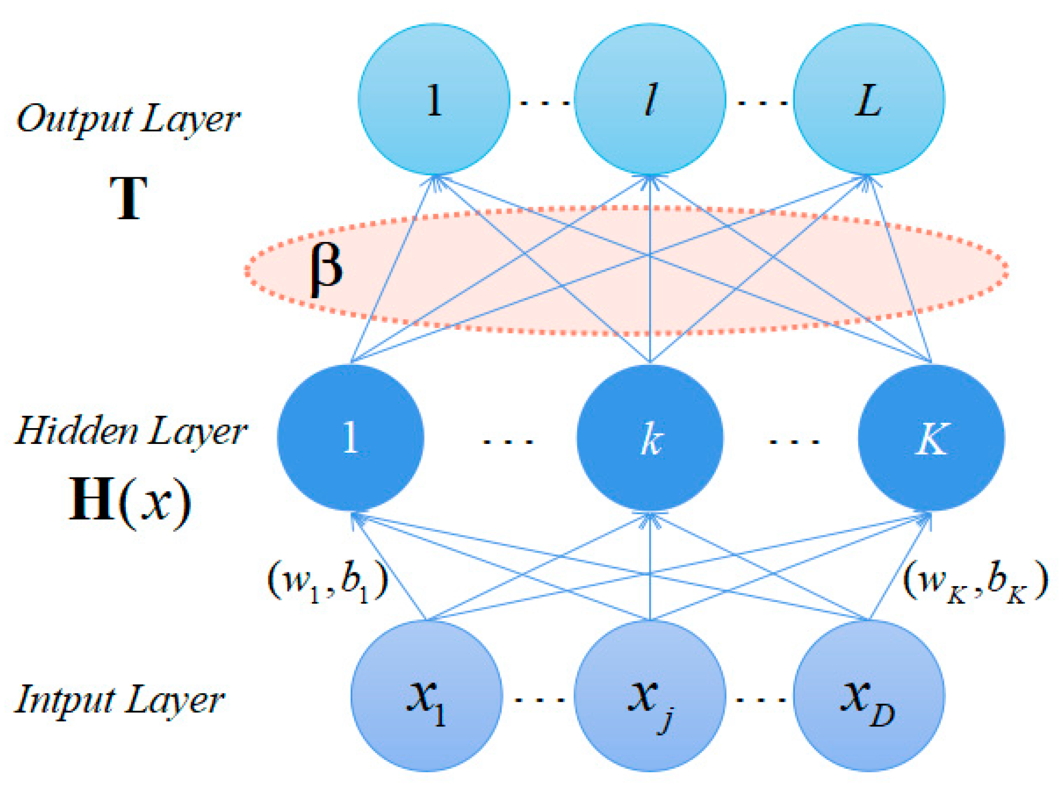
The classical zero-order TSK fuzzy classifier [50] is one of the most commonly used fuzzy classifiers, and its basic principle is as follows:

Let $\mathit{x}={[x_1,x_2,\dots ,x_n]}^{\mathrm{T}}$ be the input vector. Each component $x_i$ is a fuzzy linguistic variable, ${\mathit{\mu }}_{{\mathit{A}}_i^k}(x_i)(i=1,2,\dots ,n,k=1,2,\dots ,K)$ is each component’s corresponding membership function, and ${\mathit{A}}_i^k$ ($k=1,2,\dots ,K$) is the input vector $x_i$ in the $k$ fuzzy subsets under three rules. Then, in the $kth$ fuzzy rule, the output is $y_{}^k$. The expression is:

$$\begin{gathered} \mathrm{Rule} k: \mathrm{If} x_1 \mathrm{is} {\mathit{A}}_1^k \mathrm{And} x_2 \mathrm{is} {\mathit{A}}_2^k \mathrm{And} \dots x_n \mathrm{is} {\mathit{A}}_n^k, \mathrm{then} \\ {y}_{}^k=p_0^k,k=1,2,\dots ,K. \end{gathered}$$

where Rule $k$ represents the first $k$ rule and is the fuzzy connection operator, $K$ is the total number of fuzzy rules, and $p_0^k$ represents the first $k$ output of the fuzzy rules.

According to [51,52,53], after a series of processing on the input vector, the final output of the TSK fuzzy classifier can be expressed as:

$$y_0=\frac{{\displaystyle \sum _{k=1}^K{\mu }^k(x)}{p}_0^k}{{\displaystyle \sum _{k^{\prime }=1}^K{\mu }^{k^{\prime }}(x)}}={\displaystyle \sum _{k=1}^K{\tilde{\mu }}^k(x)}{p}_0^k={\displaystyle \sum _{k=1}^K{\mu }^k(x)}{p}_0^k$$

(1)

where the fuzzy membership function ${\mu }_{}^k(\mathit{x})$ can be written as:

$${\mu }^k(\mathit{x})={\displaystyle \prod _{i=1}^d{\mu }_{A_i^k}^k}(x_i)$$

(2)

where the normalized fuzzy membership function ${\mu }_{}^{k^{\prime }}(\mathit{x})$ can be written as:

$${\tilde{\mu }}^k(\mathit{x})=\frac{{\mu }^k(\mathit{x})}{{\displaystyle \sum _{k^{\prime }=1}^K{\mu }^{k^{\prime }}(\mathit{x})}}$$

(3)

Under normal circumstances, we use the Gaussian fuzzy membership function as the fuzzy membership function, and its expression is:

$${\mu }_{A_i^k}(x_i)=\exp (\frac{-{(x_i-c_i^k)}^2}{2{\delta }_i^k})$$

(4)

Two of the parameters, $c_i^k$ and ${\delta }_i^k$, can be calculated by using a clustering algorithm or other methods [54].

2.2. ELM

Due to the outstanding advantages of the extreme learning machine (ELM), such as fewer training parameters, fast learning speed, and strong generalization ability, its theory and application have been extensively studied in the past decade [55,56]. In simple terms, the ELM model is divided into two main stages: random feature mapping and linear parameter solving.

According to the literature [57,58], the specific principle is summarized as follows.

The network structure of ELM mainly consists of three parts: the input layer, the hidden layer, and the output layer.

Assume a given training set $\mathbf{X}=\text{{}{x}_i,t_i|x_i\in R^N,t_i\in R^L,i=1,2,3,\dots ,N\text{}}$, where ${\mathit{x}}_i$ represents the $i$th input sample, $t_i$ represents the $i$th label corresponding to each sample, and the set refers to all the training data.

The hidden layer, which is the middle layer, is fully connected to the input layer. The output of the hidden layer is $\mathbf{H}(\mathit{x})=\left[h_1(\mathit{x}),h_2(\mathit{x}),\dots ,h_K(\mathit{x})\right]$, where $h_k(\mathit{x})$ is the output of the $k$th rule layer. $K$ is the number of nodes in the hidden layer $h_k(\mathit{x})=g({\mathit{w}}_{\mathit{k}},b_k,\mathit{x})$, where $g({\mathit{w}}_{\mathit{k}},b_k,\mathit{x})$ is the activation function, ${\mathit{w}}_{\mathit{k}}$ and $b_k$ are the hidden layer node parameters. The solution of the weight value $\mathit{w}$ and the deviation $\mathit{b}$ is complete.

The output of the single hidden layer feedforward neural network ELM is $f_K(\mathit{x})={\displaystyle \sum _{k=1}^K{\beta }_k{h}_k(\mathit{x})}=\mathbf{H}(\mathit{x})\mathsf{\beta }$, where $\mathsf{\beta }={[{\mathit{\beta }}_1,{\mathit{\beta }}_2,\dots ,{\mathit{\beta }}_K]}_{}^{\mathrm{T}}$ is the output weight of the hidden layer ($K$ nodes) and the output layer (L nodes, $L\ge 1$). We can evaluate the training error with $\mathbf{H}\mathsf{\beta }$ and sample label $\mathbf{T}$ by minimizing their square difference. The objective function is $\min {\Vert \mathbf{H}\mathsf{\beta }-\mathbf{T}\mathsf{\Vert }}_{}^2,\mathsf{\beta }\in R_{}^{K*L}$, that is, the weight ($\mathsf{\beta }$) connecting the hidden layer and the output layer is solved by minimizing the approximate square difference. The solution that minimizes the objective function is the optimal solution. When the training error is minimized, the output weight $\mathsf{\beta }$ is solved.

The network structure of the ELM is shown in Figure 1.

3. Our Model

In this study, we constructed an individual thermal comfort model that considers the effects of two different materials on human comfort and combines information from the different environments. With the constructed model, the mechanism of the impact of different environmental factors on human thermal comfort was investigated. First, in this study, the original dataset from environments with two different materials (a wooden environment and a brick-concrete environment) was obtained under real laboratory conditions, their information was then preprocessed, and the features were determined. Second, this model was constructed by not only retaining the classification advantage of the training samples from a single view, but also considering the impact of the characteristics of different materials on an individual’s thermal comfort. The entire training model was optimized based on this, which was a difficulty of this study.

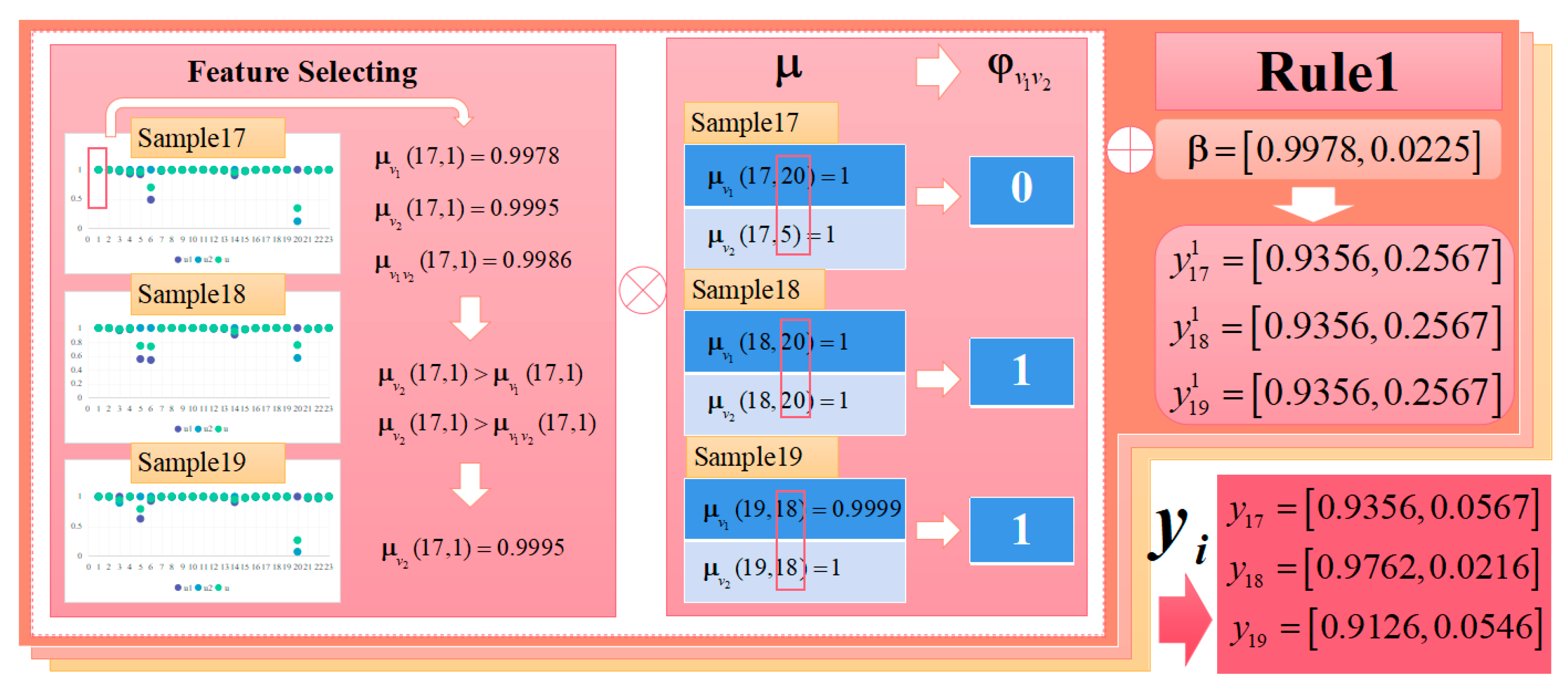
3.1. Construction of the Membership Function under the Joint View

It may be impossible to accurately predict the impact of a certain environment on the comfort of a human body from a certain view for the following reasons: the number of sample features under a single material view for constructing a thermal comfort model is small, and its importance is difficult to predict and express. Moreover, there is uncertainty in the selection of features, and predictions are often one-sided and subjective. In this study, information compensation from different views is used in the training feature preprocessing stage to avoid the subjective influence of characteristics on individual thermal comfort from a single material view; the model’s interpretability at the source training sample level is also addressed. The fuzzy membership function can represent the decision-making degree of the training features for different materials on the training results. However, the degree of independent decision making can only reflect the feeling of comfort from a single material view, and the impact of the feature information from two different views on human comfort often cannot be fully considered. Therefore, it is necessary to jointly consider two views and integrate the decision-making levels of different materials from multiple views to construct a more reasonable individual comfort model.

First, we divide $C$ equally spaced fuzzy partitions. Cluster center $a_r^{}$ falls within one of the determined partitions. In this study, a Gaussian membership function is used to obtain the degree of membership. Set $C=7$, $a_r\in (\frac{r-1}{7},\frac{r}{7}),(r=1,2,\dots ,7)$, i.e., seven fuzzy partitions, $GMF1$, $GMF2$, $GMF3$, $GMF4$, $GMF5$, $GMF6$, $GMF7$, to be equally spaced. The linguistic definitions are ‘extremely low’, ‘very low’, ‘low’, ‘medium’, ‘high’, ‘very high’, and ‘extremely high’, respectively.

Second, according to (2), the membership function of two independent views is solved separately as $u_{v_1}(x_{ij})$ and $u_{v_2}(x_{{}_{ij}}^{{}^{\prime }})$.

$$u_{v_1}(x_{ij})=\exp (-{(x_{ij}-a_{r_1})}^2/2{\sigma }_r^2)$$

(5)

$$u_{v_2}(x_{{}_{ij}}^{{}^{\prime }})=\exp (-{(x_{{}_{ij}}^{{}^{\prime }}-a_{r_2}^{{}^{\prime }})}^2/2{\sigma }_r^{{}^{\prime }2})$$

(6)

where $i=1,2,\dots ,n;j=1,2,\dots ,d;a_r\in (\frac{r-1}{7},\frac{r}{7}),r=1,2,\dots ,7$.

Third, the membership functions of two separate views are fused in this study, and the semantic partitions that best match the characteristics of each sample under two separate views are selected. In other words, the values of the Gaussian membership function under two separate views $u_{v_1}{}_{-}\max (x_{ij},r_1)$ and $u_{v_2}{}_{-}\max (x_{ij},r_2)$ and a maximum Gaussian membership function value matrix for each feature ${\mathsf{\mu }}_{v_1}$.${\mathsf{\mu }}_{v_2}$ are selected. The membership function value matrix under the joint view ${\mathsf{\mu }}_{v_1}{}_{v_2}$ is constructed, and its expression is

$${\mathsf{\mu }}_{v_1}(i,j)={\displaystyle \prod _{r_1=1}^{C_1}{u}_{v_1}{}_{-}\underset{j{r}_1}{\max }(x_{ij})}$$

(7)

$${\mathsf{\mu }}_{v_2}(i,j)={\displaystyle \prod _{r_2=1}^{C_2}{u}_{v_2}{}_{-}\underset{j{r}_2}{\max }(x_{ij}^{{}^{\prime }})}$$

(8)

$${\mathsf{\mu }}_{v_1}{}_{v_2}(i,j)=\sqrt{{\displaystyle \prod _{r_1=1}^{C_1}{u}_{v_1}{}_{-}\underset{j{r}_1}{\max }(x_{ij})}·{\displaystyle \prod _{r_2=1}^{C_2}{u}_{v_2}{}_{-}\underset{j{r}_2}{\max }(x_{ij}^{{}^{\prime }})}}$$

(9)

where $i=1,2,\dots ,N$ and $j=1,2,\dots ,D$; $C_1$ is the number of equally spaced fuzzy partitions under the first view $r_1=1,2,\cdots ,C_1$; and $C_2$ is the number of equally spaced fuzzy partitions under the second view $r_2=1,2,\cdots ,C_2$.

3.2. Construction of the Decision Coefficient Matrix

The decision coefficient matrix is an important component for feature selection. To fully consider the impact of information from two different material views on individual thermal comfort, a method to construct a decision coefficient matrix under the joint view ${\mathsf{\phi }}_{v_1{v}_2}$ is proposed in this study by comparing the important feature options under the two views.

When calculating the membership function using the joint view, the maximum membership function value matrix of each feature of the training sample under each independent view ${\mathsf{\mu }}_{v_1}$ and ${\mathsf{\mu }}_{v_2}$ is obtained. In the feature domain, the effective feature that contributes the most to information decision-making in each sample under two single views is obtained. We consider the corresponding relationship between the effective training features under two views; that is, when a certain feature is an effective feature for the two different materials, we believe that the feature is effective in improving the classification performance of the model. Then, we choose to retain this feature; otherwise, we discard this feature. For example, from the view of two materials, the most effective feature of the same $i$ sample is the $j$-dimensional feature, which means that the maximum membership function value of the $j$-dimensional feature (${\mathsf{\mu }}_{v_1}(i,j)$, ${\mathsf{\mu }}_{v_2}(i,j)$) is greater than other characteristics of the sample. Then, we can indicate that the $j$-dimensional feature is the most important feature in information decision-making under the two views, and we select this feature to construct the decision coefficient matrix. As a result, we not only retain the characteristic information of each sample under each single view but also integrate different characteristics of the two materials, thereby optimizing the final decision-making effect.

As shown in Figure 2, the decision coefficient matrix under the first material view is ${\mathsf{\phi }}_{v_1}$, and ${\mathsf{\phi }}_{v_1}$ is the matrix based on ${\mathsf{\mu }}_{v_1}$. The values of the obtained matrix are 0 or 1. The feature with the maximum membership function value of each sample is marked as 1. The decision coefficient matrix ${\mathsf{\phi }}_{v_2}$ of the second material view is constructed in a similar manner.

Therefore, we combine the feature selection matrix under the joint view ${\mathsf{\phi }}_{v_1{v}_2}$, which is expressed as:

$${\mathsf{\phi }}_{v_1{v}_2}={\left(\begin{array}{ccc}{\mathsf{\phi }}_{v_1}(1,1)\otimes {\mathsf{\phi }}_{v_2}(1,1)& \dots & {\mathsf{\phi }}_{v_1}(1,K)\otimes {\mathsf{\phi }}_{v_2}(1,K)\\ ⋮& \ddots & ⋮\\ {\mathsf{\phi }}_{v_1}(D,1)\otimes {\mathsf{\phi }}_{v_2}(D,1)& \cdots & {\mathsf{\phi }}_{v_1}(D,K)\otimes {\mathsf{\phi }}_{v_2}(D,K)\end{array}\right)}_{D\times K}$$

(10)

where $j=1,2,\dots ,D$, $k=1,2,\dots ,K$, $K$ is the number of rules, and ${\mathsf{\phi }}_{v_1{v}_2}$ is based on two single view decision coefficient matrices ${\mathsf{\phi }}_{v_1}$, ${\mathsf{\phi }}_{v_2}$. In other words, if the maximum value of the membership function is the same feature to form the corresponding matrix, then it is set to 1; otherwise, it is set to 0.

In [59], the decision coefficient matrix $\mathsf{\phi }$ is a matrix for feature selection through random partitioning and random combination, ensuring the interpretability of the fuzzy rules in the hidden layer. In [60], information entropy is determined by the method of information gain from 0 to 1 for each matrix, each element is assigned as a random initial value, and then features are selected according to a certain ratio. These methods are all effective methods for a single dataset. This study fully considers the advantages of information supplementation and important features between the two views for the dual-view classification task. Therefore, the two-view decision coefficient matrix constructed in this study contains the characteristics of the source training samples from two views. This is also one of the innovations of this study.

3.3. Output Rules

The expression of output rule $W$ is:

$$W(i,k)={\displaystyle \prod _{j=1}^D\mathsf{\mu }(i,j)·\mathsf{\phi }}(j,k)$$

(11)

where $i=1,2,\dots ,N;j=1,2,\dots ,D;k=1,2,\dots ,K$.

The selection of features is very important when outputting rules. Different features have different effects on the final classification performance. Therefore, the selection of important eigenvalues is critical. For each feature, the performance of the maximum membership function value under two single views ${\mathsf{\mu }}_{v_1}(i,j)$ and ${\mathsf{\mu }}_{v_2}(i,j)$ and the maximum membership function value under the joint view ${\mathsf{\mu }}_{v_1}{}_{v_2}(i,j)$ is considered and compared. The more advantageous maximum membership function value is selected for the fuzzy rule calculation. This includes the following situations:

Situation 1: ${\mathsf{\mu }}_{v_1}(i,j)>{\mathsf{\mu }}_{v_1}{}_{v_2}(i,j)>{\mathsf{\mu }}_{v_2}(i,j)$

The maximum membership function value under the first view is chosen when using the fuzzy rule calculation. For a certain feature, the value of the maximum membership function under the first view is greater than the value of the membership function under the joint view, and the value of the membership function under the joint view is greater than the value of the maximum membership function under the second view. Therefore, this feature can better reflect the comfort level of the individual from the first view, indicating that the contribution of this feature to the final decision is relatively large under the first view. The expression of output rules is as follows:

$$W_{ik}={\displaystyle \prod _{j=1}^D{\mathsf{\mu }}_{v_1}(i,j)·{\mathsf{\phi }}_{v_1{v}_2}(j,k)}$$

(12)

where $i=1,2,\dots ,N;j=1,2,\dots ,D;k=1,2,\dots ,K$.

Situation 2: ${\mathsf{\mu }}_{v_2}(i,j)>{\mathsf{\mu }}_{v_1}{}_{v_2}(i,j)>{\mathsf{\mu }}_{v_1}(i,j)$

Similar to situation 1, if the maximum membership function value of a certain feature from the second view is the largest and the feature performance is the best, then the maximum membership function value of situation 2 is chosen. The expression of output rule is as follows:

$$W_{ik}={\displaystyle \prod _{j=1}^D{\mathsf{\mu }}_{v_2}(i,j)·{\mathsf{\phi }}_{v_1{v}_2}(j,k)}$$

(13)

where $i=1,2,\dots ,N;j=1,2,\dots ,D;k=1,2,\dots ,K$.

Situation 3: ${\mathsf{\mu }}_{v_1}(i,j)>{\mathsf{\mu }}_{v_1}{}_{v_2}(i,j)$ AND ${\mathsf{\mu }}_{v_2}(i,j)>{\mathsf{\mu }}_{v_1}{}_{v_2}(i,j)$

If the value of the maximum membership function of a certain feature from two separate views is greater than the value of the membership function under the joint view, the feature can better reflect the degree of comfort of the individual under the two separate views. This indicates that for this feature, the two independent views have a relatively large impact on the final decision. In this case, the average value of the two views is used to calculate the fuzzy rule. The expression is described as follows:

$$W_{ik}={\displaystyle \prod _{j=1}^D\frac{{\mathsf{\mu }}_{v_1}(i,j)+{\mathsf{\mu }}_{v_2}(i,j)}{2}\times }{\mathsf{\phi }}_{v_1{v}_2}(j,k)$$

(14)

where $i=1,2,\dots ,N;j=1,2,\dots ,D;k=1,2,\dots ,K$.

Situation 4: ${\mathsf{\mu }}_{v_1}(i,j)<{\mathsf{\mu }}_{v_1}{}_{v_2}(i,j)$ AND ${\mathsf{\mu }}_{v_2}(i,j)<{\mathsf{\mu }}_{v_1}{}_{v_2}(i,j)$

If for a certain feature, the value of the membership function of the joint view is greater than the value of the maximum membership function of two separate views, the degree of comfort of the individual can be better determined through the joint view, since the joint view is integrated after considering the factors of the two views. With superior performance, the output rule can be expressed as:

$$W_{ik}={\displaystyle \prod _{j=1}^D{\mathsf{\mu }}_{v_1}{}_{v_2}(i,j)·}{\mathsf{\phi }}_{v_1{v}_2}(j,k)$$

(15)

where $i=1,2,\dots ,N;j=1,2,\dots ,D;k=1,2,\dots ,K$.

Thus, for output rule $W$, we ensure the attributes of important features by selecting the value corresponding to the most advantageous view, which is chosen through the comparison of each membership function value. Effective information is also retained by the decision coefficient matrix ${\mathsf{\phi }}_{v_1{v}_2}$ under the joint view. Figure 3 shows the method of decision coefficient matrix under the joint view. This method integrates the feature information from two views, resulting in universal applicability for dual views, which is one of the important innovations in this paper.

3.4. The Algorithm

The algorithm adopted in the proposed model is shown in Algorithm 1, and Figure 4 shows the working flowchart of the TMV-TSK-FC model.

Algorithm 1: Training Algorithm Of TMV-TSK-FC

Input: The training set ${\mathbf{X}}_{v_1}={[{\mathit{x}}_1,{\mathit{x}}_2,\dots ,{\mathit{x}}_N]}^T$, ${\mathbf{X}}_{v_2}={[{\mathit{x}}_1^{{}^{\prime }},{\mathit{x}}_2^{{}^{\prime }},\dots ,{\mathit{x}}_N^{{}^{\prime }}]}^T$;           The corresponding class label set $\mathbf{T}={(t_1,t_2,\dots ,t_N)}^T$

Step 1: Compute the values of Gaussian membership functions           Step 1(a): Compute the values of Gaussian membership functions for each view                          $u=\exp (-{(x_{ij}-a_k)}^2/2{\sigma }_k^2)$           Step 1(b): Compute the maximum Gaussian membership functions for each view and the mix view                          ${\mathsf{\mu }}_{v_1}(i,j)={\displaystyle \prod _{r_1=1}^{C_1}{u}_{v_1}{}_{-}\underset{j{r}_1}{\max }(x_{ij})}$                          ${\mathsf{\mu }}_{v_2}(i,j)={\displaystyle \prod _{r_2=1}^{C_2}{u}_{v_2}{}_{-}\underset{j{r}_2}{\max }(x_{ij}^{{}^{\prime }})}$                ${\mathsf{\mu }}_{v_1}{}_{v_2}(i,j)=\sqrt{{\displaystyle \prod _{r_1=1}^{C_1}{u}_{v_1}{}_{-}\underset{j{r}_1}{\max }(x_{ij})}·{\displaystyle \prod _{r_2=1}^{C_2}{u}_{v_2}{}_{-}\underset{j{r}_2}{\max }(x_{ij}^{{}^{\prime }})}}$

Step2: Compute the projection matrix                           ${\mathsf{\phi }}_{v_1{v}_2}={\left(\begin{array}{ccc}{\mathsf{\phi }}_{v_1}(1,1)\otimes {\mathsf{\phi }}_{v_2}(1,1)& \dots & {\mathsf{\phi }}_{v_1}(1,K)\otimes {\mathsf{\phi }}_{v_2}(1,K)\\ ⋮& \ddots & ⋮\\ {\mathsf{\phi }}_{v_1}(D,1)\otimes {\mathsf{\phi }}_{v_2}(D,1)& \cdots & {\mathsf{\phi }}_{v_1}(D,K)\otimes {\mathsf{\phi }}_{v_2}(D,K)\end{array}\right)}_{D\times K}$

Step 3:      For$i\leftarrow 1ton$      Choose optimized membership functions to compute the following value of the premise of each fuzzy rule                          $W_{ik}={\displaystyle \prod _{j=1}^D{\mathsf{\mu }}_{v_1}{}_{v_2}(i,j)·}{\mathsf{\phi }}_{v_1{v}_2}(j,k)$           Step 3(a): If ${\mathsf{\mu }}_{v_1}(i,j)>{\mathsf{\mu }}_{v_1}{}_{v_2}(i,j)>{\mathsf{\mu }}_{v_2}(i,j)$, Then $W_{ik}={\displaystyle \prod _{j=1}^D{\mathsf{\mu }}_{v_1}(i,j)·{\mathsf{\phi }}_{v_1{v}_2}(j,k)}$           Step 3(b): If ${\mathsf{\mu }}_{v_2}(i,j)>{\mathsf{\mu }}_{v_1}{}_{v_2}(i,j)>{\mathsf{\mu }}_{v_1}(i,j)$, Then $W_{ik}={\displaystyle \prod _{j=1}^D{\mathsf{\mu }}_{v_2}(i,j)·{\mathsf{\phi }}_{v_1{v}_2}(j,k)}$           Step 3(c): If ${\mathsf{\mu }}_{v_1}(i,j)>{\mathsf{\mu }}_{v_1}{}_{v_2}(i,j),{\mathsf{\mu }}_{v_2}(i,j)>{\mathsf{\mu }}_{v_1}{}_{v_2}(i,j)$, Then $W_{ik}={\displaystyle \prod _{j=1}^D\frac{{\mathsf{\mu }}_{v_1}(i,j)+{\mathsf{\mu }}_{v_2}(i,j)}{2}·}{\mathsf{\phi }}_{v_1{v}_2}(j,k)$           Step 3(d): If ${\mathsf{\mu }}_{v_1}(i,j)<{\mathsf{\mu }}_{v_1}{}_{v_2}(i,j),{\mathsf{\mu }}_{v_2}(i,j)<{\mathsf{\mu }}_{v_1}{}_{v_2}(i,j)$, Then $W_{ik}={\displaystyle \prod _{j=1}^D{\mathsf{\mu }}_{v_1}{}_{v_2}(i,j)·}{\mathsf{\phi }}_{v_1{v}_2}(j,k)$      End For

Step 4: Construct a rule layer output matrix H       $\mathbf{H}={[{\mathit{w}}_1,{\mathit{w}}_2,\dots ,{\mathit{w}}_K]}_{N\times K}^{\mathrm{T}}$

Output:      The prediction function of TMV-TSK-FC: $\mathbf{Y}=\mathbf{H}·\mathsf{\beta }$

3.5. Time Complexity Analysis

The time complexity of the algorithm includes six parts: the construction of the membership function under the joint view, the construction of the decision coefficient matrix under the joint view, the output of the selection rule, the construction of the decision coefficient matrix $\mathbf{H}$ under the joint view, the construction of matrix $\mathsf{\beta }$ and the result output. The corresponding time complexities are $O(7DK)$, $O(DK)$, $O(DK)$, $O(7N{D}^{2}K)$, $O(K^3+NK+NL)$, and $O(NKL)$, respectively. According to the order of magnitude, the final time complexity is $O(7DK+7N{D}^{2}K+K^3+NKL)$. For the thermal comfort model, the number of features and the number of rules are relatively small. When the test sample N is large, the time complexity of the model can be simplified as follows: $O(7N{D}^{2}K)$. It indicates a linear relationship with sample N and is part of a reasonable range.

4. Experiment and Discussion

4.1. Experimental Setup

The dataset in this study was obtained by field research in the laboratory. The sampling location was in Zhangjiagang City, which is located between latitudes 31°43′12″–32°02′ and longitudes 120°21′57″–120°52′, and the southern part has a tropical wet climate. All subjects lived in Zhangjiagang City for one year or more and were fully adapted to the local climatic conditions. The subjects were divided into two groups for data collection in April 2020 and April 2021. The basic information of the subjects, including sampling conditions, physical environment, physiological parameters, subjective perception, and self-assessment were measured and analyzed statistically. The numbers of subjects in the two groups were 48 and 109.

a.

Experimental procedure

The subjects received 30 min of training before participating in the experiment to ensure that they were aware of how to perform physiological measurements. They were also required to complete an experiment for approximately 160 min (30 min in the preparation room, 60 min of sampling time in the first stage, 10 min of rest, and 60 min of sampling time in the second stage). The experimental process was as follows. First, each subject received the sampling information form in the preparation room; the basic information was completed, and sampling conditions were collected. After sitting still for approximately 30 min, the subject entered experimental chamber 1 (stage 1). To adapt to this indoor environment, the physiological parameters of the subjects and the physical parameters of the indoor environment were simultaneously recorded by the staff; then, the subjects completed the subjective perception and self-assessment evaluation forms. The staff reviewed this information to ensure correctness. Next, subjects left experimental chamber 1 for 10 min, during which time the staff thoroughly ventilated and cleaned this chamber. Then, the subject entered experimental chamber 2 (stage 2). For minutes 100–130, reading or online status was resumed; after minutes 130–160, the staff again recorded physiological parameters, physical environment parameters, subjective perception, and self-assessment evaluation forms. Once the tests in the two stages were completed and the inspection was correct, the staff left the sampling room. To exclude the effect of the experimental sequence on the feeling of comfort, the experimental cabins using material 1 and material 2 were divided into Groups A and B for simultaneous experiments, respectively. Figure 5 shows the experimental process.

b.

Characteristics and labels

According to [23,24,25,26,27,28,29,30,31,32,33,34,35,36], individual thermal comfort models constructed in the past mostly collected information from indoor and outdoor physical environments and human body responses as features information. The number of subjects surveyed was usually limited, ranging from one to a few in these models because of the difficulties in recruiting subjects, the long sampling period, etc. The limitation related to an insufficient number of surveyed subjects in previous models was overcome in this study by surveying a larger number of subjects, and a comprehensive classification of the characteristics that affect individual thermal comfort was conducted to obtain a more comprehensive data sample. The selected features included six categories (i.e., basic information, sampling conditions, physiological parameters, physical environment, environmental perception, and self-assessment), which are summarized in

Table 1. Selected features for the development of TMV-TSK-FC personal thermal comfort models.

Category	Characteristics
Basic information	Information such as gender, height, age, new city metabolism, clothing thermal resistance, and BMI
Sampling conditions	The weather of the day, the materials of the sampling chamber, the opening and closing of the windows, etc.
Physiological parameters	High pressure, low pressure, pulse, perspiration rate, and multipart body surface temperature
Physical environment	Indoor and outdoor air temperature, relative humidity, indoor surface temperature, and black bulb temperature
Environmental awareness	Subjective feelings such as environmental coldness and heat, comfort, and expectation
Self-assessment	Health, mood, performance, fatigue, etc.

.

Since the thermal sensation vote (TSV) is currently the most widely accepted standard in comfort studies, the thermal sensation of an individual is evaluated based on the ASHRAE scale. The sample labels with individual thermal sensation vote values of −1, 0, 1 are defined as comfortable, and the sample labels with values less than −1 or greater than 1 are defined as uncomfortable, thereby achieving a binary classification task, as shown in Figure 6.

To obtain more valuable training samples during sample preprocessing, we tracked the comfort feeling of the same subject in both experimental cabins. When the same subject felt the same in both experimental cabins, we selected the sample. Otherwise, the training sample was discarded. The processed datasets were grouped to obtain a sample on the feeling of indoor environment comfort.

Table 2. Dataset descriptions.

Groups	Visual Angle	No. of Selected Samples	No. of Total Samples	No. of Features	No. of Classes
Data 1 *	Timber	27	48	23	2
	Concrete	27	48	23	2
Data 2 *	Timber	76	109	34	2
	Concrete	76	109	34	2

* Data 1 is the dataset collected in April 2020, and data 2 is the dataset collected in April 2021.

provides a detailed description of the two experimental datasets. Seventy-five percent of the samples in each dataset were used for training, and the remainder were used for testing.

c.

Parameter settings

The main parameters of this experiment include the number of fuzzy rules $K$, number of clustering centers $C$, and coefficient $\lambda$, which can be set manually in advance. The detailed settings are shown in

Table 3. Experimental parameter settings.

Parameter	Value
$\mathrm{Number} \mathrm{of} \mathrm{fuzzy} \mathrm{rules} K$	55~60
$\mathrm{Number} \mathrm{of} \mathrm{cluster} \mathrm{centers} C_1$$C_2$	7
$\lambda$	(0, 0.1)
$\eta$	(0, 0.1)

.

4.2. Description of the Comparison Algorithm

In this study, we used the four classical optimization algorithms with DBN [61], QI-TSK [60], and the KEEL software (KEEL can be downloaded from http:www.keel.es/download.php (accessed on 30 March 2022)), as comparison algorithms to evaluate and verify the rationality and superiority of the proposed model. Knowledge extraction based on evolutionary learning (KEEL) is a machine learning software based on Java that integrates a variety of classical algorithms and their corresponding optimization algorithms. It mainly includes classification algorithms, regression algorithms, and semi-supervised learning algorithms. The four classical optimization algorithms adopted are JADE-C, SADE-C, GFS-ADABOOST-C, and GFS-MAXLOGITBOOST-C. Among the above algorithms, DBN is the classic nonfuzzy machine learning algorithm, QI-TSK is the optimized TSK algorithm, JADE-C and SADE-C are the classic nonfuzzy algorithms in the KEEL software, and GFS-ADABOOST-C and GFS-MAXLOGITBOOST are the classic nonfuzzy algorithms in the KEEL software. Therefore, the performance of the proposed model, TMV-TSK-FC, can be comprehensively observed by comparison with the classical DBN algorithm, the optimized TSK algorithm, and the classical fuzzy and nonfuzzy algorithms in the KEEL software. The detailed algorithm descriptions are presented in

Table 4. Algorithm descriptions.

Algorithms	Main Descriptions of Compared Algorithms	Main Descriptions of TMV-TSK-FC
DBN	(1) Hierarchical structure with multiple hidden layers; only the nodes of adjacent layers are connected. (2) The process of feature learning has better feature expression.	(1) Dataset input: bi-view information input. (2) Feature selection and rule output: By constructing a membership function from a joint view, comparing the size of its membership value, select the membership function value that contributes the most to decision making, so that the feature information of the two views can be effectively processed. Fusion, and by constructing a decision coefficient matrix, select the features that are closely related to information decision making for rule output. (3) Fuzzy rules: TMV-TSK-FC has high usability and interpretability.
QI-TSK	(1) The basic building blocks of QI-TSK-fc (td > 1) are all composed of optimized zero-order TSK fuzzy classifiers. Each base building unit is aligned with the adjacent base building unit. (2) Fuzzy rules and features have high interpretability. (3) The algorithm does not need to iterate.
JADE-C	(1) The optimal mutation strategy is randomly selected. (2) Self-adaptive parameter control and control parameters.
SADE-C	For a single training set, there is no feature selection ability. Influence the mutation strategy of the next generation according to the success rate of the recorded mutation strategy.
GFS-ADABOOST-C	(1) Use a single training set to train different fuzzy classifiers. (2) High classification performance, no feature filtering, but long training time.
GFS-MAXLOGITBOOST-C	(1) The loss function is derived by maximizing the log-likelihood function. (2) Optimize in a way similar to Newton iteration.

. In addition, comparative experiments were conducted in this study to investigate the rationality of optimization measures such as the construction of membership functions and the construction of the decision coefficient matrix from the fusion view.

4.3. Performance Evaluation

The learning algorithm proposed in this study is compared with the classical optimization algorithms (JADE-C, SADE-C, GFS-ADABOOST-C, and GFS-MAXLOGITBOOST-C) in the software. The membership function and the research method of constructing the decision coefficient matrix from the view of fusion were compared and verified.

(1)

Classification performance and generalization performance

According to Figure 7, the classification and generalization performance of TMV-TSK-FC on the above two datasets are observed. Based on the training structure of the first dataset, QI-TSK and GFS-ADABOOST-C have good training accuracies, and TMV-TSK-FC is able to perform classification as well as the other algorithms. Based on the training structure of the second dataset, which has a larger number of samples in the dataset, the use of TMV-TSK-FC with the fusion of the two material views improves the classification accuracy compared with the other algorithms. In addition, Figure 7 also shows that TMV-TSK-FC has good generalization performance. Since TMV-TSK-FC effectively integrates the feature information of two views and selects features relating closely to the information decision for output rule, it has better generalization performance. It is worth noting that the output of the TMV-TSK-FC training intermediate layer, the output of each fuzzy rule, and the output of the final fuzzy classifier are all interpretable.

(2)

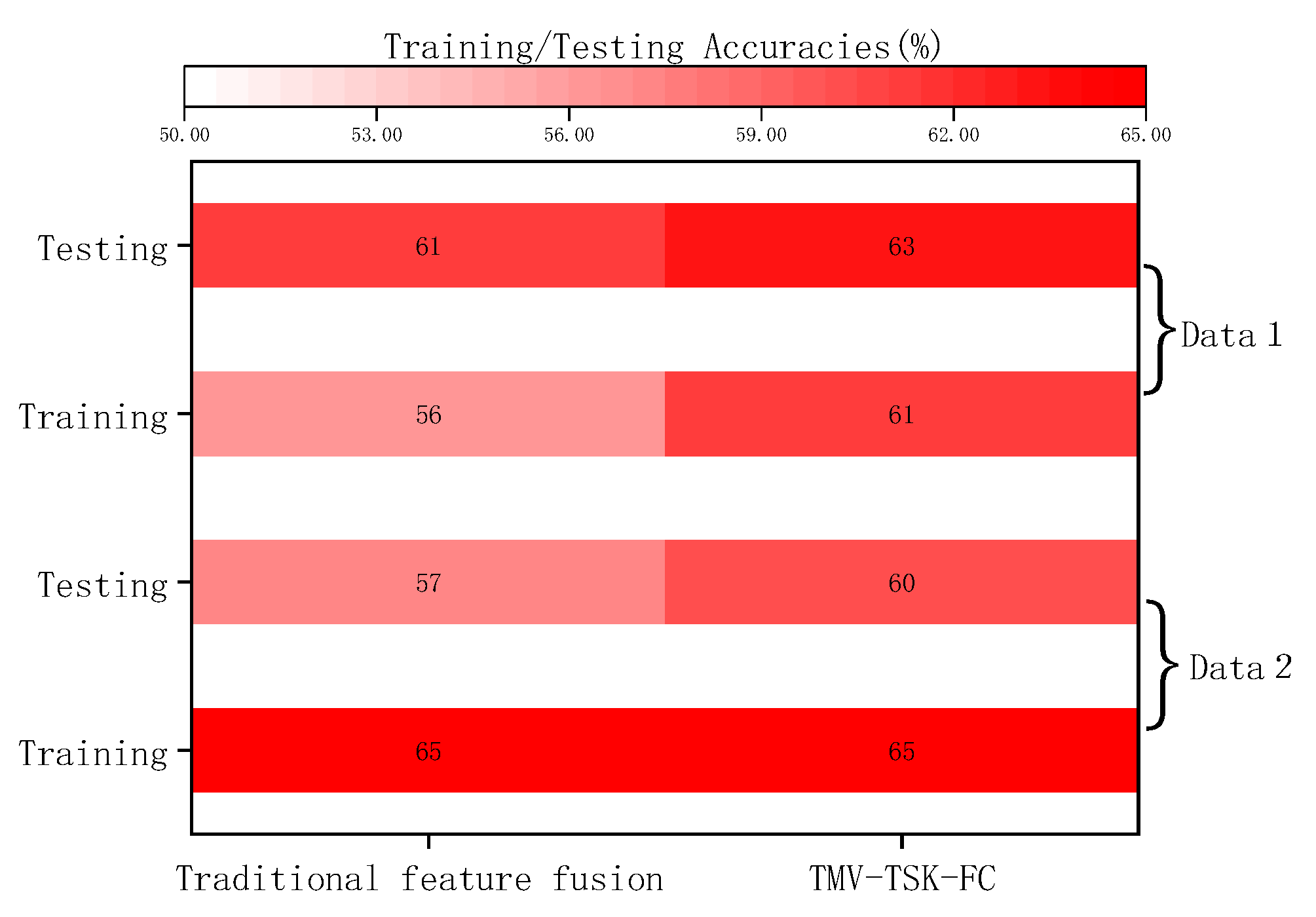
Optimization method for feature selection

Figure 8 shows the effect of TMV-TSK-FC on the classification and generalization performance before and after feature selection optimization. First, the membership function value of each feature under the optimized joint view is solved. The method used to obtain the solution takes the arithmetic mean of the membership function value of the feature from the two views based on the fuzzy center. From the view of classification accuracy, the optimized method indeed provides TMV-TSK-FC with a better classification ability. This advantage may be due to the selection of dominant features that have a large contribution to decision-making under both views, which improves the performance of classification and generalization.

(3)

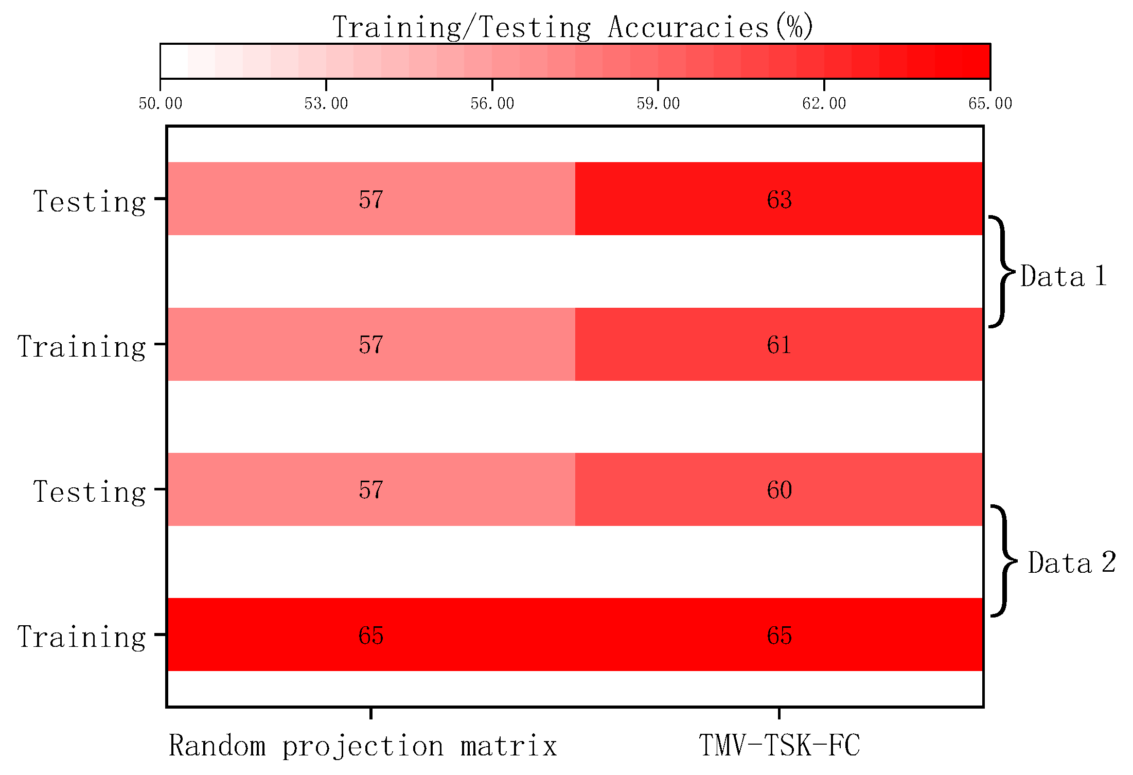
The optimization method of the decision coefficient matrix

To further verify the rationality of the proposed method with respect to the construction of the decision coefficient matrix, a method of calculating the arithmetic mean of the decision coefficient matrix under two single views is used in this study as a comparison method. The information gain method determines the information entropy, assigns a random initial value from 0 to 1 to each element, and then randomly selects features according to a ratio of 70%. The purpose of this study is to observe the impact of the above two optimization methods on the classification and generalization performance. According to Figure 9, the classification and generalization performance of TMV-TSK-FC by constructing the decision coefficient matrix optimized in this paper is generally higher than that of the average decision coefficient matrix. The experimental results show that the method of optimizing the decision coefficient matrix proposed in this paper is reasonable. Therefore, the decision coefficient matrix can be applied to retain the feature information that contributes significantly to the decision under two views, by which means the inherent information of the two independent views can be fully considered by the final decision. In addition, the learning efficiency, classification, and generalization performance of the fuzzy classifier can be improved.

4.4. Semantic Interpretability Analysis

To prove the good semantic interpretation ability of the proposed TMV-TSK-FC classification model, semantic interpretation is performed on fuzzy rules and the model output from two views. Taking the first fuzzy rule in each view as an example, the parameters before and after each rule and the Gaussian membership function are given. Three sample points are randomly selected to represent the merging process of the two fuzzy rules.

Table 5. Antecedent and consequent parameters and the Gaussian membership function.

Sample1	Feature 1	Feature 2	Feature 3	...	${\mathit{p}}_0^1$
Rule1 in view1	$e_{}^{-\frac{1}{2}{(\frac{x-0.1032}{0.1314})}_{}^2}$	$e_{}^{-\frac{1}{2}{(\frac{x-0.1866}{0.0589})}_{}^2}$	$e_{}^{-\frac{1}{2}{(\frac{x-0.3804}{-2.0578})}_{}^2}$	…	0.7236
Rule1 in view2	$e_{}^{-\frac{1}{2}{(\frac{x-0.0454}{-1.4152})}_{}^2}$	$e_{}^{-\frac{1}{2}{(\frac{x-0.2045}{-0.1759})}_{}^2}$	$e_{}^{-\frac{1}{2}{(\frac{x-0.3110}{0.2101})}_{}^2}$	...	0.2489

shows the parameters of the context and the Gaussian membership function. Figure 10 shows the interpretability of the feature selections and outputs of the fuzzy rules.

Table 5 shows the output of the first rule under the first view. The Gaussian membership function distribution is used for fuzzy division. Taking the first sample as an example, the cluster center points of the Gaussian fuzzy membership functions of each feature are randomly located in seven partitions, the center point of feature 1 is 0.1032, and the center point of feature 2 is 0.1866.... Then, the membership function value is generated, and the rule output $p_0^1$ is 0.7236.

Figure 10 shows the process of feature selection, decision coefficient matrix generation, rule generation, and the final output of the three sample points under the first rule. Taking the 17th sample as an example, its maximum membership function value is 0.9995 under the second view, so this membership function value is selected. The maximum membership function value of sample 17 under the first view appears at the position of the 20th feature, whereas it is the fifth feature under the second view; therefore, they are not the same feature, and So its decision coefficient matrix output is 0. It was inferred to belong to the first class since its output value of the first category is much larger than that of the second category.

5. Conclusions

In this study, an individual thermal comfort model, TMV-TSK-FC, was developed and applied to observe the effects of two materials on an individual’s thermal comfort based on the TSK fuzzy classification theory and the ELM extreme learning machine theory.

In constructing the model, decision-making levels from two different views were fused to reflect the inherent characteristic information of each sample in a more reasonable manner and improve the classification performance of the model. The decision-making level strategy under construction of the joint view was adopted for feature selection so that TMV-TSK-FC can not only satisfy the interpretability but also share the feature information under two views. In this study, we also adopted the method of constructing the decision coefficient matrix under the joint view to determine the view with good decision-making ability, which is based on whether the maximum decision-making degree values of the two views correspond to the same training feature. Compared with several traditional non-fuzzy classifiers (i.e., DBN, JADE-C, SADE-C, GFS-ADABOOST-C, and GFS-MAXLOGITBOOST-C), the experimental results indicated that the proposed TMV-TSK-FC showed good classification performance and generalization performance. Compared with several related state-of-the-art single view fuzzy classifier (i.e., classical 0-order TSK fuzzy system and QI-TSK-FC), the training accuracies (testing accuracies) of TMV-TSK-FC are improved by 3–11% (2–9%). In addition, the experiments also proved good interpretability of TMV-TSK-FC. Facing more practical scenarios, future work should discuss how to quickly obtain the hyperparameter combination and expand the two views for multi-view learning or multi-task learning.

References

1. Zhang, J. Integrating IAQ control strategies to reduce the risk of asymptomatic SARS-CoV-2 infections in classrooms and open plan offices. Sci. Technol. Built. Environ. 2020, 26, 1013–1018. [Google Scholar] [CrossRef]
2. Tham, K.W.; Willem, H.C. Room air temperature affects occupants’ physiology, perceptions and mental alertness. Build. Environ. 2010, 45, 40–44. [Google Scholar] [CrossRef]
3. Zhang, F.; de Dear, R.; Candido, C. Thermal comfort during temperature cycles induced by direct load control strategies of peak electricity demand management. Build. Environ. 2016, 103, 9–20. [Google Scholar] [CrossRef] [Green Version]
4. Wargocki, P.; Wyon, D.P.; Sundell, J.; Clausen, G.; Fanger, P.O. The effects of outdoor air supply rate in an office on perceived air quality, sick building syndrome (SBS) symptoms and productivity. Indoor Air 2000, 10, 222–236. [Google Scholar] [CrossRef]
5. Wyon, D.P. The effects of indoor air quality on performance and productivity. Indoor Air 2004, 14, 92–101. [Google Scholar] [CrossRef]
6. Fisk, W.J.; Rosenfeld, A.H. Estimates of improved productivity and health from better indoor environments. Indoor Air 1997, 7, 158–172. [Google Scholar] [CrossRef]
7. Allen, J.G.; Macnaughton, P.; Laurent, J.G.C.; Flanigan, S.S.; Eitland, E.S.; Spengler, J.D. Green buildings and health. Curr. Environ. Health Rep. 2015, 2, 250–258. [Google Scholar] [CrossRef] [PubMed] [Green Version]
8. Klepeis, N.E.; Nelson, W.C.; Ott, W.R.; Robinson, J.P.; Tsang, A.M.; Switzer, P.; Behar, J.V.; Hern, S.C.; Engelmann, W.H. The national human activity pattern survey (NHAPS): A resource for assessing exposure to environmental pollutants. J. Expo. Anal. Environ. Epidemiol. 2001, 11, 231–252. [Google Scholar] [CrossRef] [Green Version]
9. Fanger, P.O. Thermal comfort analysis and applications in environmental engineering. In Thermal Comfort Analysis and Applications in Environmental Engineering; McGraw-Hill: New York, NY, USA, 1970. [Google Scholar]
10. Yang, B.; Li, X.; Liu, Y.; Chen, L.; Guo, R.; Wang, F.; Yan, K. Comparison of models for predicting winter individual thermal comfort based on machine learning algorithms. Build. Environ. 2022, 215, 108970. [Google Scholar] [CrossRef]
11. Wang, Z.; de Dear, R.; Luo, M.; Lin, B.; He, Y.; Ghahramani, A.; Zhu, Y. Individual difference in thermal comfort: A literature review. Build. Environ. 2018, 138, 181–193. [Google Scholar] [CrossRef]
12. Yang, B.; Li, X.; Hou, Y.; Meier, A.; Cheng, X.; Choi, J.; Wang, F.; Wang, H.; Wagner, A.; Yan, D.; et al. Non-invasive (non-contact) measurements of human thermal physiology signals and thermal comfort/discomfort poses—A review. Energy Build. 2020, 224, 110261. [Google Scholar] [CrossRef]
13. Cheung, T.; Schiavon, S.; Parkinson, T.; Li, P.; Brager, G. Analysis of the accuracy on PMV—PPD model using the ASHRAE Global Thermal Comfort Database II. Build. Environ. 2019, 153, 205–217. [Google Scholar] [CrossRef] [Green Version]
14. De Dear, R.J.; Brager, G.S. Developing an adaptive model of thermal comfort and preference. ASHRAE Trans. 1998, 104, 145–167. [Google Scholar]
15. Zhou, X.; Xu, L.; Zhang, J.; Niu, B.; Luo, M.; Zhou, G.; Zhang, X. Data-driven thermal comfort model via support vector machine algorithms: Insights from ASHRAE RP-884 database. Energy Build. 2020, 211, 109795. [Google Scholar] [CrossRef]
16. Rupp, R.F.; de Dear, R.; Ghisi, E. Field study of mixed-mode office buildings in Southern Brazil using an adaptive thermal comfort framework. Energy Build. 2018, 158, 1475–1486. [Google Scholar] [CrossRef]
17. Luo, M.; Cao, B.; Damiens, J.; Lin, B.; Zhu, Y. Evaluating thermal comfort in mixed-mode buildings: A field study in a subtropical climate. Build. Environ. 2015, 88, 46–54. [Google Scholar] [CrossRef]
18. Zhang, R.; Liu, D.; Shi, L. Thermal-comfort optimization design method for semi-outdoor stadium using machine learning. Build. Environ. 2022, 215, 108890. [Google Scholar] [CrossRef]
19. Irshad, K.; Habib, K.; Kareem, M.W.; Basrawi, F.; Saha, B.B. Evaluation of thermal comfort in a test room equipped with a photovoltaic assisted thermo-electric air duct cooling system. Int. J. Hydrogen Energy 2017, 42, 26956–26972. [Google Scholar] [CrossRef] [Green Version]
20. Irshad, K.; Algarni, S.; Jamil, B.; Ahmad, M.T.; Khan, M.A. Effect of gender difference on sleeping comfort and building energy utilization: Field study on test chamber with thermoelectric air-cooling system. Build. Environ. 2019, 152, 214–227. [Google Scholar] [CrossRef]
21. Megri, A.C.; El Naqa, I. Prediction of the thermal comfort indices using improved support vector machine classifiers and nonlinear kernel functions. Indoor Built Environ. 2016, 25, 6–16. [Google Scholar] [CrossRef] [Green Version]
22. Choi, J.; Yeom, D. Study of data-driven thermal sensation prediction model as a function of local body skin temperatures in a built environment. Build. Environ. 2017, 121, 130–147. [Google Scholar] [CrossRef]
23. Li, D.; Menassa, C.C.; Kamat, V.R. Personalized human comfort in indoor building environments under diverse conditioning modes. Build. Environ. 2017, 126, 304–317. [Google Scholar] [CrossRef]
24. Chaudhuri, T.; Zhai, D.; Soh, Y.C.; Li, H.; Xie, L. Random forest based thermal comfort prediction from gender-specific physiological parameters using wearable sensing technology. Energy Build. 2018, 166, 391–406. [Google Scholar] [CrossRef]
25. Salehi, B.; Ghanbaran, A.H.; Maerefat, M. Intelligent models to predict the indoor thermal sensation and thermal demand in steady state based on occupants’ skin temperature. Build. Environ. 2020, 169, 106579. [Google Scholar] [CrossRef]
26. Katić, K.; Li, R.; Zeiler, W. Machine learning algorithms applied to a prediction of personal overall thermal comfort using skin temperatures and occupants’ heating behavior. Appl. Ergon. 2020, 85, 103078. [Google Scholar] [CrossRef] [PubMed]
27. Ma, N.; Chen, L.; Hu, J.; Perdikaris, P.; Braham, W.W. Adaptive behavior and different thermal experiences of real people: A Bayesian neural network approach to thermal preference prediction and classification. Build. Environ. 2021, 198, 107875. [Google Scholar] [CrossRef]
28. Aryal, A.; Becerik-Gerber, B. Thermal comfort modeling when personalized comfort systems are in use: Comparison of sensing and learning methods. Build. Environ. 2020, 185, 107316. [Google Scholar] [CrossRef]
29. Wu, Y.; Liu, H.; Li, B.; Kosonen, R.; Wei, S.; Jokisalo, J.; Cheng, Y. Individual thermal comfort prediction using classification tree model based on physiological parameters and thermal history in winter. Build. Simul. 2021, 14, 1651–1665. [Google Scholar] [CrossRef]
30. Zhang, W.; Wu, Y.; Calautit, J.K. A review on occupancy prediction through machine learning for enhancing energy efficiency, air quality and thermal comfort in the built environment. Renew. Sustain. Energy. Rev. 2022, 167, 112704. [Google Scholar] [CrossRef]
31. Irshad, K.; Khan, A.I.; Irfan, S.A.; Alam, M.M.; Almalawi, A.; Zahir, M.H. Utilizing artificial neural network for prediction of occupants thermal comfort: A case study of a test room fitted with a thermoelectric air-conditioning system. IEEE Access 2020, 8, 99709–99728. [Google Scholar] [CrossRef]
32. Kim, J.; Schiavon, S.; Brager, G. Personal comfort models—A new paradigm in thermal comfort for occupant-centric environmental control. Build. Environ. 2018, 132, 114–124. [Google Scholar] [CrossRef]
33. Arakawa Martins, L.; Soebarto, V.; Williamson, T.; Pisaniello, D. Personal thermal comfort models: A deep learning approach for predicting older people’s thermal preference. Smart Sustain. Built Environ. 2022, 11, 245–270. [Google Scholar] [CrossRef]
34. Liu, S.; Schiavon, S.; Das, H.P.; Jin, M.; Spanos, C.J. Personal thermal comfort models with wearable sensors. Build. Environ. 2019, 162, 106281. [Google Scholar] [CrossRef] [Green Version]
35. Cosma, A.C.; Simha, R. Machine learning method for real-time non-invasive prediction of individual thermal preference in transient conditions. Build. Environ. 2019, 148, 372–383. [Google Scholar] [CrossRef]
36. Lu, S.; Wang, W.; Lin, C.; Hameen, E.C. Data-driven simulation of a thermal comfort-based temperature set-point control with ASHRAE RP884. Build. Environ. 2019, 156, 137–146. [Google Scholar] [CrossRef]
37. Yang, B.; Cheng, X.; Dai, D.; Olofsson, T.; Li, H.; Meier, A. Real-time and contactless measurements of thermal discomfort based on human poses for energy efficient control of buildings. Build. Environ. 2019, 162, 106284. [Google Scholar] [CrossRef]
38. Xie, J.; Li, H.; Li, C.; Zhang, J.; Luo, M. Review on occupant-centric thermal comfort sensing, predicting, and controlling. Energy Build. 2020, 226, 110392. [Google Scholar] [CrossRef]
39. De Dear, R.; Xiong, J.; Kim, J.; Cao, B. A review of adaptive thermal comfort research since 1998. Energy Build. 2020, 214, 109893. [Google Scholar] [CrossRef]
40. Burnard, M.D.; Kutnar, A. Wood and human stress in the built indoor environment: A review. Wood Sci. Technol. 2015, 49, 969–986. [Google Scholar] [CrossRef]
41. Kaplan, R.; Kaplan, S. The Experience of Nature: A Psychological View; Cambridge University Press: Cambridge, UK, 1989. [Google Scholar]
42. Tsunetsugu, Y.; Miyazaki, Y.; Sato, H. Physiological effects in humans induced by the visual stimulation of room interiors with different wood quantities. J. Wood Sci. 2007, 53, 11–16. [Google Scholar] [CrossRef]
43. Tsunetsugu, Y.; Miyazaki, Y.; Sato, H. Visual effects of interior design in actual-size living rooms on physiological responses. Build. Environ. 2005, 40, 1341–1346. [Google Scholar] [CrossRef]
44. Ulrich, R.S. Effects of interior design on wellness: Theory and recent scientific research. Health Care. Inte. Des. 1991, 3, 97–109. [Google Scholar]
45. Ulrich, R.S.; Robert, F.S.; Barbara, D.L.; Evelyn, F.; Milest, M.A.; Zelsont, M. Stress recovery during exposure to natural and urban environments. Environ. Psychol. 1991, 11, 201–230. [Google Scholar] [CrossRef]
46. Zhang, X.; Lian, Z.; Wu, Y. Human physiological responses to wooden indoor environment. Physoi. behav. 2017, 174, 27–34. [Google Scholar] [CrossRef] [PubMed]
47. Zhao, T.; Chen, C.; Cao, H. Evolutionary self-organizing fuzzy system using fuzzy-classification-based social learning particle swarm optimization. Inf. Sci. 2022, 606, 92–111. [Google Scholar] [CrossRef]
48. Zhao, T.; Chen, C.; Cao, H.; Dian, S.; Xie, X. Multiobjective Optimization design of interpretable evolutionary fuzzy systems with type self-organizing learning of fuzzy sets. IEEE Trans. Fuzzy Syst. 2022, 3207318. [Google Scholar] [CrossRef]
49. Zhao, T.; Cao, H.; Dian, S. A self-organized method for a hierarchical fuzzy logic system based on a fuzzy autoencoder. IEEE Trans. Fuzzy Syst. 2022, 3165690. [Google Scholar] [CrossRef]
50. Jiang, Y.; Chung, F.L.; Ishibuchi, H.; Deng, Z.; Wang, S. Multitask TSK fuzzy system modeling by mining intertask common hidden structure. IEEE Trans. Cybern. 2015, 45, 548–561. [Google Scholar]
51. Wang, S.; Chung, F.L.; Hongbin, S.; Dewen, H. Cascaded centralized TSK fuzzy system: Universal approximator and high interpretation. Appl. Soft. Comput. 2005, 5, 131–145. [Google Scholar] [CrossRef]
52. Takagi, T.; Sugeno, M. Fuzzy identification of systems and its application to modeling and control. Trans. System. Man. Cybern. 1985, 15, 116–132. [Google Scholar] [CrossRef]
53. Deng, Z.; Cao, L.; Jiang, Y.; Wang, S. Minimax probability TSK fuzzy system classifier: A more transparent and highly interpretable classification model. IEEE Trans. Fuzzy Syst. 2015, 23, 813–826. [Google Scholar] [CrossRef]
54. Bayindir, R.; Gok, M.; Kabalci, E.; Kaplan, O. An intelligent power factor correction approach based on linear regression and ridge regression methods. In Proceedings of the 2011 10th International Conference on Machine Learning and Applications and Workshops, Honolulu, HI, USA, 18–21 December 2011; pp. 313–315. [Google Scholar]
55. Kasun, L.L.C.; Zhou, H.; Huang, G. Representational learning with ELMs for big data. Intell. Syst. 2013, 28, 31–34. [Google Scholar]
56. Tang, J.; Deng, C.; Huang, G. Extreme learning machine for multilayer perceptron. IEEE Trans. Neural Netw. Learn. Syst. 2016, 27, 809–821. [Google Scholar] [CrossRef] [PubMed]
57. Huang, G.; Huang, G.; Song, S.; You, K. Trends in extreme learning machines: A review. Neural Netw. 2015, 61, 32–48. [Google Scholar] [CrossRef]
58. Huang, G.; Zhu, Q.; Siew, C. Extreme learning machine: Theory and applications. Neurocomputing 2006, 70, 489–501. [Google Scholar] [CrossRef]
59. Zhou, T.; Chung, F.; Wang, S. Deep TSK fuzzy classifier with stacked generalization and triplely concise interpretability guarantee for large data. IEEE Trans. Fuzzy Syst. 2017, 25, 1207–1221. [Google Scholar] [CrossRef]
60. Zhou, T.; Zhou, Y.; Gao, S. Quantitative-integration-based TSK fuzzy classification through improving the consistency of multi-hierarchical structure. Appl. Soft. Comput. 2021, 106, 107350. [Google Scholar] [CrossRef]
61. Hinton, G.E.; Osindero, S.; Teh, Y. A fast learning algorithm for deep belief nets. Neural Comput. 2006, 18, 1527–1554. [Google Scholar] [CrossRef]
Figure 1. Network Structure of the ELM.
Applsci 12 11700 g001
Figure 2. The decision coefficient matrix under the joint view.
Applsci 12 11700 g002
Figure 3. Membership function value selecting under the joint view.
Applsci 12 11700 g003
Figure 4. TMV-TSK-FC structure diagram.
Applsci 12 11700 g004
Figure 5. Experimental flow diagram.
Applsci 12 11700 g005
Figure 6. Schematic diagram of Thermal Sensation classification.
Applsci 12 11700 g006
Figure 7. Comparison between TMV-TSK-FC and the other algorithms.
Applsci 12 11700 g007
Figure 8. Comparison between TMV-TSK-FC and different feature optimization methods.
Applsci 12 11700 g008
Figure 9. Comparison between TMV-TSK-FC and different decision coefficient matrix algorithms.
Applsci 12 11700 g009
Figure 10. Antecedent and consequent parameters and the Gaussian membership function.
Applsci 12 11700 g010