
Satellite Image Super-Resolution by 2D RRDB and Edge-Enhanced Generative Adversarial Network †
1
Department of Electrical Engineering and Graduate Institute of Communication Engineering, National Chung Hsing University, Taichung 40227, Taiwan
2
Product Development Department, E-Great Technology, Miaoli 35157, Taiwan
*
Author to whom correspondence should be addressed.
†
This paper is an extended version of a paper published in ICASSP 2022–2022 IEEE International Conference on Acoustics, Speech and Signal Processing (ICASSP), 27 April 2022, Singapore.
Appl. Sci. 2022, 12(23), 12311; https://0-doi-org.brum.beds.ac.uk/10.3390/app122312311
Submission received: 10 November 2022
/
Revised: 25 November 2022
/
Accepted: 26 November 2022
/
Published: 1 December 2022
(This article belongs to the Special Issue New Trends on Machine Learning Based Pattern Recognition and Classification)
Abstract
:With the gradually increasing demand for high-resolution images, image super-resolution (SR) technology has become more and more important in our daily life. In general, high resolution is often accomplished by increasing the accuracy and density of the sensor. However, such an approach is too expensive on the design and equipment. Particularly, increasing the sensor density of satellites incurs great risks. Inspired by EEGAN, some parts of networks: Ultra-Dense Subnet (UDSN) and Edge-Enhanced Subnet (EESN) are modified. The UDSN is used to extract features and obtain high-resolution images which look clear but are deteriorated by artifacts in the intermediate stage, while the EESN is used to purify, enhance and extract the image contours and uses mask processing to eliminate the image corrupted by noise. Then, the restored intermediate image and the enhanced edge are combined to become a high-resolution image with clear contents and high authenticity. Finally, we use Kaggle open source, AID, WHU-RS19, and SpaceWill datasets to perform the test and compare the SR results among different models. It shows that our proposed approach outperforms other state-of-the-art SR models on satellite images.
1. Introduction
Recently, high-resolution (HR) satellite images have become important in many applications [1], including building extraction, environmental disaster assessment, small object detection, and urban planning. However, because of high costs of hardware and limitations of current technology, the observed HR images usually have incomplete spatial and temporal coverage. Moreover, the resolution does not satisfy the required standard, making them unable to meet the gradually-growing applications and demand of the general public, which has caused a negative impact on the accuracy of subsequent computer vision tasks. As we know, super-resolution (SR) technology on images provides an effective and low-cost approach of reconstructing HR images from easily available and relatively low-resolution (LR) images. Thus, this paper mainly focuses on how to generate high-quality HR satellite images in a cost-effective direction.
In recent years, SR models based on Generative Adversarial Networks (GANs) [2], such as Super Resolution GAN (SRGAN) [3] and Enhanced Super Resolution GAN (ESRGAN) [4] have been proposed and also have promising performance in enhancing noiseless or noisy LR images. The above models consist of generators and discriminators. Both sub-networks are composed of deep convolutional neural networks (CNNs). The dataset which contains LR and HR image pairs is required to train the model. Then the generator produces the HR image from an input (LR) image, and the discriminator decides if the generated image is just an enlarged LR image or a real HR image. After training with sufficient data and time, the generator is able to output synthetic (fake) HR images which are supposed to be similar to real HR images, while the discriminator is not capable of distinguishing between fake and true images.
The satellite imagery covers a wide area, including various ground scenes. In addition, the resolution of satellite images is much lower than general images, and it is also susceptible to several effects such as ultra-telephoto imaging, atmospheric disturbances, and equipment noise. This further increases the difficulty on the edge restoration with details and sharpness from LR input images. Therefore, the conspicuous outline of the ground target is more worth pursuing than the actual texture details inside the object. In the past few years, various shallow and deep learning-based reconstruction methods have been proposed to improve the resolution of satellite images. Especially, the residual learning strategy is applied to build a deeper CNN for computer vision tasks and makes the results amazing. For the image SR problem, these methods aim to predict the residual image (relative to the input image) rather than the target HR image, and the methods based on residual learning and their variants have been proven effective. Although the image generated looks very realistic, the image content is excessively eroded due to the global optimization strategy. As a result, the SR image may be inconsistent with the actual HR image and a large number of false or smooth edges may appear.
We are inspired by the EEGAN [5] and EESRGAN [6] and use EEGAN as the basic framework to propose a feasible infrastructure. For the two sub-networks in the generator, a combination of residual-in-residual dense block and two-dimensional topology (i.e., 2D-RRDB) is used. Compared with the conventional RRDB [4], this 2D architecture with additional diagonal connections can lead to better gradient optimization on the links between different routes and provide more possibilities for information conversion. In other words, more connected paths can be obtained using the same number of layers through the diagonal links. That means by increasing the density of dense blocks connection over the traditional 1D infrastructure, we can effectively overcome the information propagation disappearance, gradient disappearance and training difficulty problems caused by increasing the layer depth.
Moreover, in the light of the use of the same approach to compute the perceptual loss for the entire image (e.g., we use the same features on the foreground, background, and edges), the proposed model needs to include new losses and learn the information for smaller features (e.g., the texture of the building). We use the feature map before the activation layer of VGG19 [7] to compute both the perceptual loss and edge perceptual loss, which can assist in generating more visually consistent results and sharper edges. Moreover, since satellite images usually cause more noise than ordinary images, the Canny algorithm [8] is required to be used for edge extraction to help the generator create distinguishable and clearer edge maps. In the end, we used several popular and publicly available datasets for training and testing, and compared the results with other state-of-the-art SR models. We not only consider PSNR but also look for several evaluation indices to evaluate the performance. As a result, we learned that our model can generate satellite images which look more natural and visually close to real images.
The paper is an extension of our previous work in [9]. Compared to the original work, we add the following substantive new contents. First, we describe related works to this topic in Section 2, including a review of existing methods on image super-resolution, an introduction of Generative Adversarial Network (GAN), edge detection algorithms, and perceptual loss. Furthermore, in Section 3.1 and Section 3.4, we perform a thorough ablation study on two sub-networks (UDSN, EESN) of the generator, edge detection algorithms, and loss functions to compare the performances. Moreover, in Section 4, we conduct more experiments on two additional data sets, including WHU-RS19 and SpaceWill data sets to prove the robustness of the proposed approach.
The rest of paper is organized as follows. In Section 2, we give an introduction of image super-resolution and review some existing state-of-the-art SR methods and several possible techniques that could be used to improve the SR performance. Then we describe the proposed approach in Section 3, including the modifications in two sub-networks in the generator, edge extraction module, and perceptual loss on edges. Section 4 shows the experimental results and discusses the performance comparison on several publicly available satellite image data sets. Finally, we draw the conclusions in Section 5.
2. Related Works
Deep learning (e.g., CNN) [10,11,12,13,14] has been widely used in image SR reconstruction, and the SR performance has been significantly improved due to the powerful function of deep neural networks. Therefore, we focus on exploring deep neural network methods to solve SR problems.
2.1. Image SR
CNN is widely used in image SR, and the early image SR model was proposed by Dong et al. [15]. They use CNNs to achieve the end-to-end mapping between LR and HR images. Then Shi et al. improved the previous SRCNN and proposed FSRCNN [16], which does not need to enlarge the image size outside the network. By adding a shrinkage layer and an expansion layer on the network, some small layers can be used to replace a large layer at the same time, and FSRCNN has a greater speed increase than SRCNN. Inspired by this work, other researchers proposed to adopt other deep learning architectures, such as RNN, Residual CNNs [12] and GANs [2] to solve single image super-resolution (SISR). Among them, Ledig et al. [3] introduced an architecture “SRResNet” inspired by ResNet [17], which preserves the batch normalization within the original residual block. This makes their model significantly reduce memory and allow adaptation to several ideas introduced for image deblurring. Similarly, Lim et al. [12] proposed their EDSR (Enhanced Depth Super Resolution) model. This model effectively reduces the memory space by removing the batch normalization (BN) layer in the residual block in SRResNet, and uses this space to expand the size of the model, thereby achieving significant performance improvements.
Because of the specialty (e.g., the large size of spatial dimension) of satellite images, some SR methods are specifically developed for satellite images. In [18], Kawulok et al. indicate the characteristics of training data have a large impact on the accuracy of a reconstructed image. In [19], Shermeyer et al. investigate the application of SR techniques to satellite images and the effects on object detection performance. Wei et al. [20] employ a deep segmented residual CNN approach to analyze the SR performance of a single satellite image. Rout et al. [21] report considerable improvements in SR of remote sensing imagery are achieved by using supervised models in a reinforcement learning framework. In [22], Zhu et al. claimed using a simple down-sampling approach with a fixed kernel to create training images works fine on synthetic data, but does not perform well on real satellite images. In addition, some examples for recent SR methods based on CNN and Generative Adversarial Network (GAN) are [23,24], respectively. Recently, Tewari et al. [25] introduced a unique loss function and a new image reconstruction method to enable the SR model to be executed on a low-power device for satellite environments.
2.2. GAN Methods for Image SR
GAN [2] is a deep learning model which is composed of two networks. One is the Discriminating Network and the other is the Generative Network. Inspired by GAN, researchers have conducted active research on it. Recently, some effective and practical techniques have been applied to low-level computer vision tasks, including image SR [26]. For instance, Ledig et al. [3] proposed a realistic single-image SR using GAN (SRGAN), which uses adversarial loss to push the reconstruction result to the natural image. Wang et al. [4] improved the generator on the basis of SRGAN, and the RRDB network architecture is proposed. The BN layer is removed from the architecture, and the idea of relativity GAN is borrowed to let the discriminator predict the authenticity of the image instead of “whether it is a fake image”. Finally, the perceived loss is also improved. These improvements have brought better visual quality and more realistic and natural textures. Jiang et al. [5] proposed an Edge Enhanced Network (i.e., EEGAN) architecture based on GAN. This method is used to provide robust satellite image SR reconstruction and an adversarial learning strategy that is insensitive to noise. This method retains enough edge information to bring better results to the final SR image.
2.3. Edge Detection and Extraction
Edge detection is a very important image feature extraction method in the area of computer vision, and it is also relatively easy to use. We use edge detection to find a set of pixels in the image that significantly change the brightness of the pixels. The edge extraction itself is a filtering process, using different operation elements to extract different features. Each type of operand has its own characteristics. There are generally three traditional methods: Sobel operator [27,28], Laplacian operator [27,28] and Canny operator [8].
- Sobel OperatorIn target detection, Sobel operator has a better effect on image processing with more gray gradient and noise, but it is not very accurate in edge positioning (i.e., the edge of the image is more than one pixel). Therefore, the accuracy of Sobel operator is not very high.
- Laplacian OperatorSince the Laplacian method is more sensitive to noise, it is rarely used to detect edges. However, it is used to determine whether edge pixels are regarded as bright or dark areas of the image. The Laplacian is the second derivative operand, which will produce steep zero crossings at the edges. Laplacian operands are isotropic and can sharpen borders and lines in any direction.
- Canny OperatorThe best things about Canny edge detection algorithms are: (1) Detecting edges with a low error rate, which means capturing as many edges as possible in the image and as accurately as possible. (2) The detected edge should be accurately positioned at the center of the true edge. (3) A given edge in the image should be marked only once, and the noise of the image should not produce false edges wherever possible.
2.4. Perceptual Loss
The perceptual loss function is usually used to convert images among various styles. The success of the style transfer algorithm lies in the field of image generation. A very important idea has emerged here, that is, the features extracted by the CNN can be used as part of the loss function, and the image generated by a certain layer of pretrained networks can be compared. The feature map obtained from the specific layer of the network makes the semantics in the generated image and the target image more similar. The network is divided into two types: transform network and loss network. The transform network is used to convert the image, and its parameters changed, while the loss network keeps the parameters unchanged. The transformed result map, style map and content map are passed through the loss network to obtain the feature map of each layer and we can use it to calculate the loss.
General style transfer uses both style loss and content loss. As the name suggests, style loss is used to change the style of the input image, while content loss is used to preserve the content of the image. The difference between the perceptual loss functions of super-resolution and style transfer is that the SR only needs content loss. Recently, SR methods aimed at improving visual quality and added this perceptual loss function. The generated image after adding perceptual loss function is much clearer than the image generated by using only the L1 (Manhattan norm) or L2 (Euclidean norm) loss function. We add the perceptual loss function to our SR method, and find a set of results that are more in line with human vision through different parameter adjustments.
To summarize, the main contributions and advantages of our proposed approach in this work are:
- We incorporate the 2D topology into RRDB for both sub-networks in the generator to obtain extra diagonal connections to achieve better gradient optimizations among different paths to prevent the gradient vanishing and training difficulty problems.
- We try different edge detection algorithms and choose Canny approach to replace original Laplacian method to get more detailed and clear edge information.
- The new loss function (e.g., edge perceptual loss) is added into original loss function and different weighting combinations are conducted to obtain the best SR result.
- Through extensive experiments on four well-known and publicly available satellite image databases, we evaluate all compared SR models with five objective image quality metrics to show the proposed approach is able to generate SR images with better visual quality and more close to the true image.
3. Materials and Methods
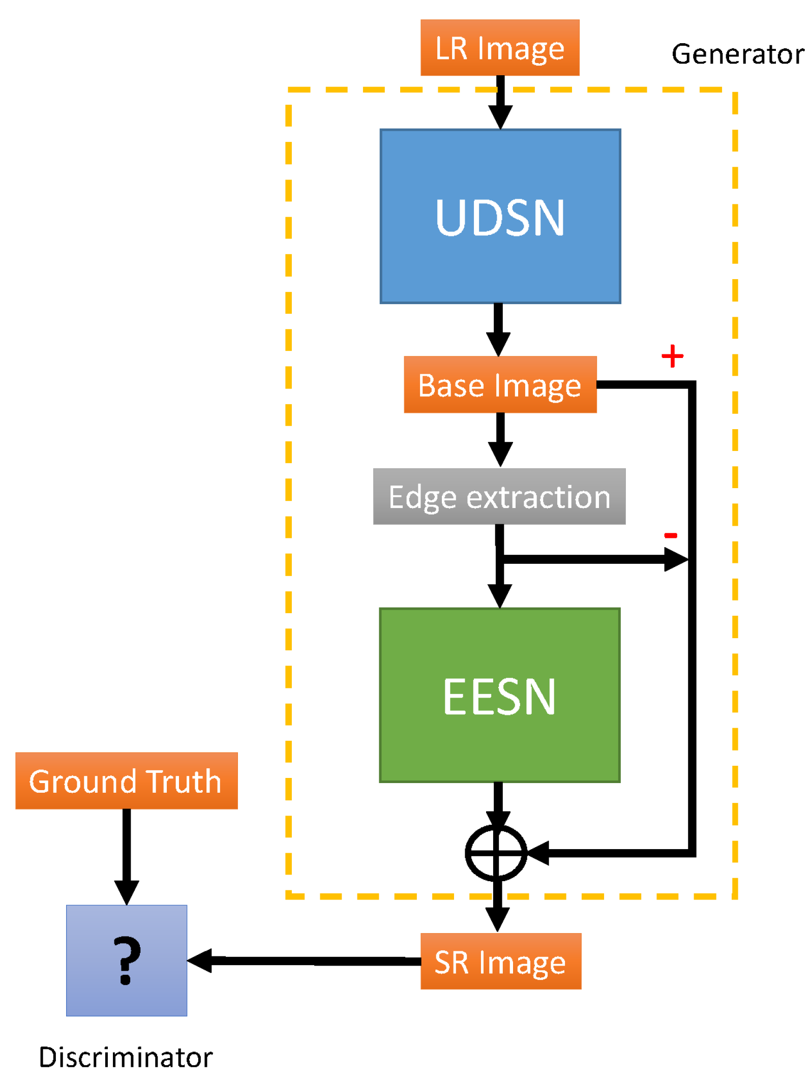
For our proposed approach, EEGAN [5] is adopted as the basic framework and some modifications are made based on it. As shown in Figure 1, we can divide the generator G into two sub-networks: ultra-dense subnet (UDSN) and edge-enhanced subnet (EESN). The UDSN is made up of several dense blocks and a reconstruction layer which can be used to generate intermediate HR image, while the EESN is used to enhance the edges extracted from the intermediate SR image by removing artifacts and noise. Then, the clean edges from EESN will replace the noisy edges in the intermediate SR image and output the final SR image. A perceptual loss function is tried to be added into the model to enhance visual quality [29,30,31]. We find a set of parameters that can achieve better performance through the process of parameter adjustments in conducted experiments. The obtained HR images are also compared with the ones generated by other SR models. We will describe more details in the following subsections.
3.1. Generator Networks
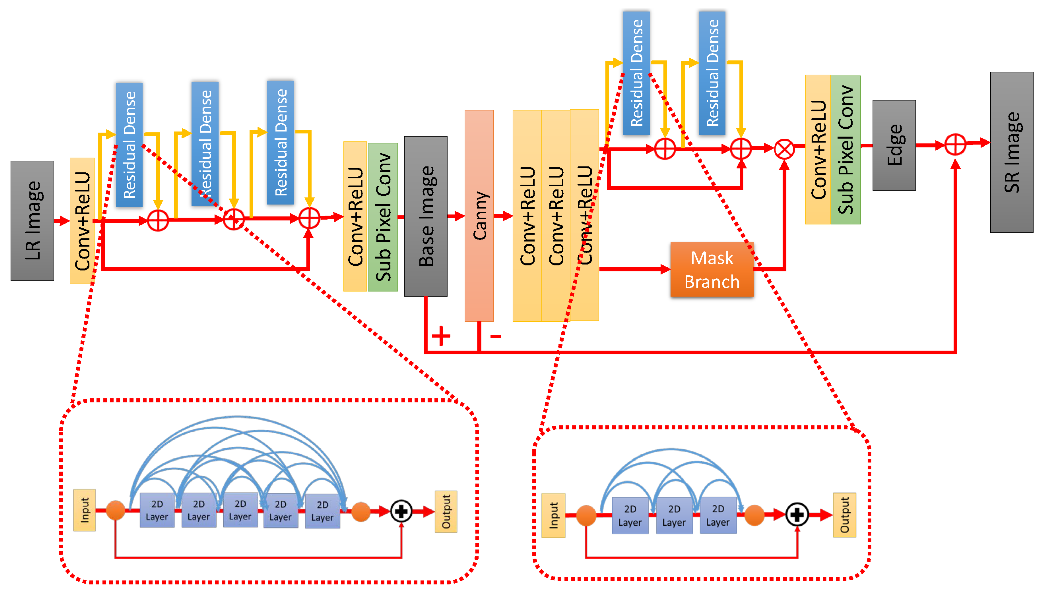
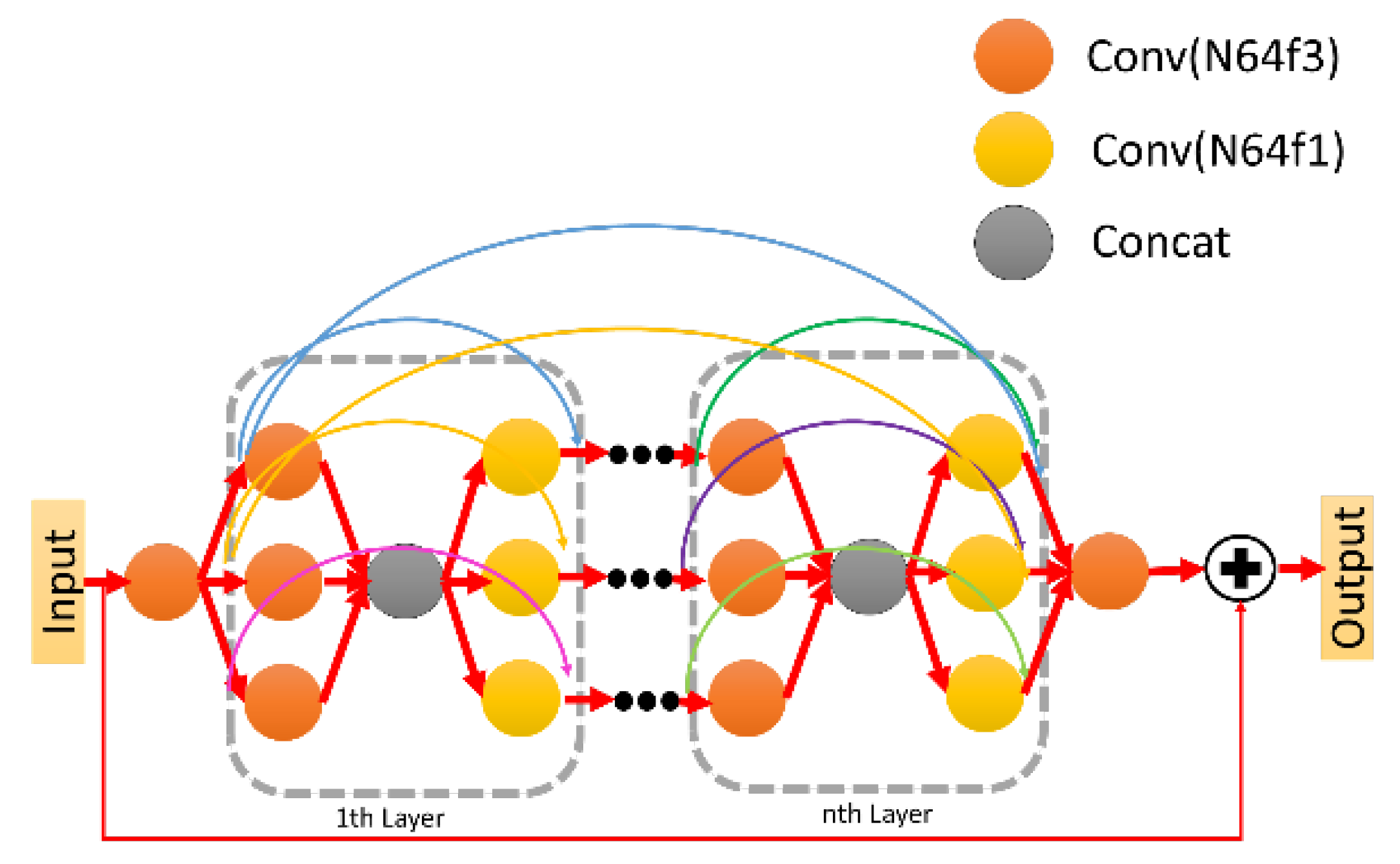
As shown in Figure 2, the UDSN is first modified to generate intermediate HR images, and then the dense subnet branch of the EESN is also modified. Regarding the UDSN, we replace the original dense block [32] with two different blocks (i.e., residual dense block (RDB) and RRDB), and use two different convolution topologies (i.e., original one-dimensional and new two-dimensional (2D) topology [5] in the convolutional layers, which is shown in Figure 3) as the choice. Through the extensive experiments, we list the best results for each of the above four combinations, as shown in Table 1. We can see it will have the best PSNR and FSIM results when the block type is RRDB with 2D-topology and the number of blocks is 3, while the number of convolutional layers in each block is 5. This means to modify the generator network architecture will output SR images that are more close to real HR images.
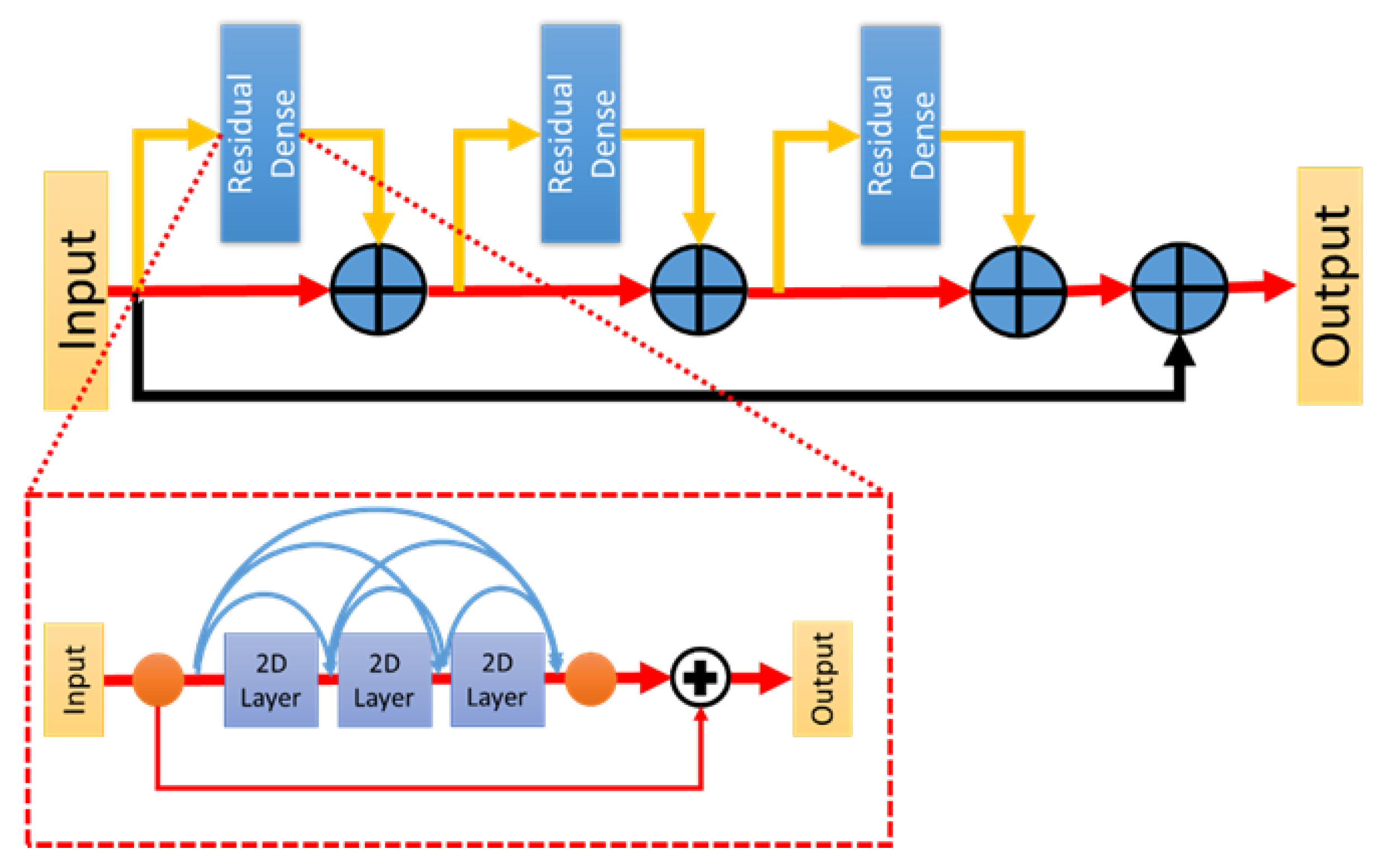
Then we use convolutional layers with 2D topology to replace the original convolution layers in the adopted RDB for the dense network branch of the EESN, as shown in Figure 4. We hope that the EESN can generate useful edge features through this network architecture. In Table 2, we test four different combinations for block types (RDB, RRDB) and convolution topologies (1D, 2D). We can find the model will have the best PSNR and SSIM values when the block type is RRDB with 2D-topology and the number of blocks is 2, while the number of convolutional layers in each block is 3.
3.2. Edge Enhancement
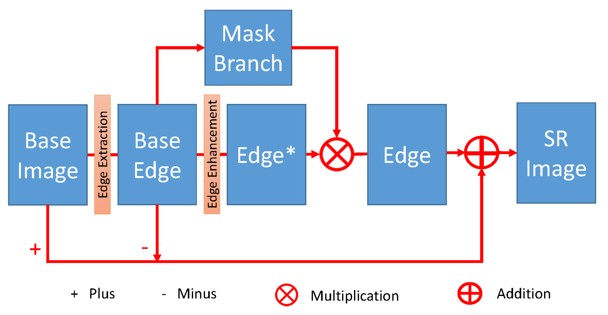
In this part, we will investigate different edge extraction algorithms used in the EESN of the generator network. Through experiments, better edge extraction algorithms are found by comparing their effects. The results are shown in Table 3. Furthermore, we adopt the Mask Branch in EEGAN [5] to suppress false edges and noise. Figure 5 shows the details of this operation. First, we use the intermediate SR image generated by the UDSN as an input (i.e., Base Image in Figure 5), and a Base Edge image is obtained through the edge extraction method, and then it is fed to two sub-networks (i.e., edge enhancement and mask branch) separately. The outputs of these two sub-networks eventually combine (via multiplication) to produce the image with sharper edges. Then, the sharper edges (Edge in Figure 5) will replace the noisy edges (Base Edge in Figure 5) in the intermediate SR image and output the final SR image. In the conducted experiments, we try the Sobel and Canny methods [33]. In consequence, we find that Canny method can generate the final SR image with better performance among the three compared algorithms.
3.3. Loss Functions
At first, we create a content loss function to force the generator G to output the intermediate HR image that is supposed to be similar to the real HR image by the equation below:
where represents a set of model parameters in the generator, represents the Charbonnier penalty function [10]. As the same as [10], the compensation parameter is set to , and denote the real HR image and the intermediate HR image generated by the UDSN.
To reduce artifacts and enhance the quality of the reconstructed image, we included the pixel-based Charbonnier loss to improve the consistency of the image content between the real and generated HR images. The consistency loss function is denoted as:
where is the model parameter set as the same as mentioned before, and refer to the real HR image and the final SR image.
Then, and are both input into the discriminator to determine the authenticity of . Moreover, the discriminator is trained to minimize the adversarial loss, which can force the generator to output the reconstructed image as similar as the real HR image. The adversarial loss can be written as:
where refers to the model parameters in the discriminator, represents the input LR image, represents the generator function, and is the discriminator function to compute the probability of being the generated HR image or real HR image. In the discriminator, the generated image is expected to be classified as 0, and the real image is expected to be classified as 1. If the discriminator can correctly decide whether this is a real or generated image, then the Equation (3) will output 0, which is the smallest value. For the generator, it is expected to confuse the discriminator to make it unable to distinguish between the real image and generated image, and classify the generated image as 1.
Furthermore, we included the edge image consistency loss function, as shown in Equation (4), where is the edge image of the real HR image, and is the edge image of the generated SR image. As we know, the image consistency loss in Equation (2) helps to obtain an output with good edge information, but the edges for some objects in the image are distorted and have produced noise. Therefore, we incorporate this loss to resolve this issue. The weighting coefficient of this loss is chosen to be the same as .
Equation (5) shows the perceptual loss [34], and we incorporated the edge perceptual loss function described in Equation (6). The feature map () before the activation layer of the fine-tuned VGG19 [7] network are adopted to compute the perceptual loss and the edge perceptual loss as follows:
where represents the intermediate SR image, is the real HR image, is the edge map of the intermediate SR image, is the edge map of the real HR image, and E denotes the calculation of mean value for the difference of feature maps.
3.4. Ablation Study
To prove the feasibility of the proposed model, we conducted ablation experiments using different UDSN and EESN networks, different edge extraction methods, and adding other different loss functions. In all the ablation experiments, we used the pre-processed Kaggle data set and randomly selected 4000 images (72% training, 8% validation, and 20% testing) to conduct experiments.
As shown in Table 4, we can see that the network architecture using RRDB with two-dimensional topology convolution has significantly improved the output results. By extensive ablation experiments, we discover that for the UDSN, using the 2D-topology RRDB has the best results, where the number of residual dense blocks (RDBs) in the RRDB is 3, while the number of convolutional layers in each RDB is 5 and they are all connected in 2D-topology. For the EESN, it still shows using the 2D topology convolutional layers in the RRDB brings the best SR performance. However, the number of RDBs in the RRDB becomes 2, and the number of convolutional layers in each RDB is 3. The final decided architecture for the generator is shown in Figure 2.
Next, through experiments by using different edge extraction approaches, it is found that using Canny edge extraction (PSNR: 33.011 dB, SSIM: 0.918) method can bring better performance to the SR results than the Sobel (PSNR: 32.950 dB, SSIM: 0.906) and Laplacian (PSNR: 32.947 dB, SSIM: 0.913) methods. Finally, we sequentially add different loss functions to the original loss function. It is found that adding these losses into the model will yield a better performance for the final output SR image. The best performance happens when we add , , and into the original loss function.
3.5. Discriminator Networks
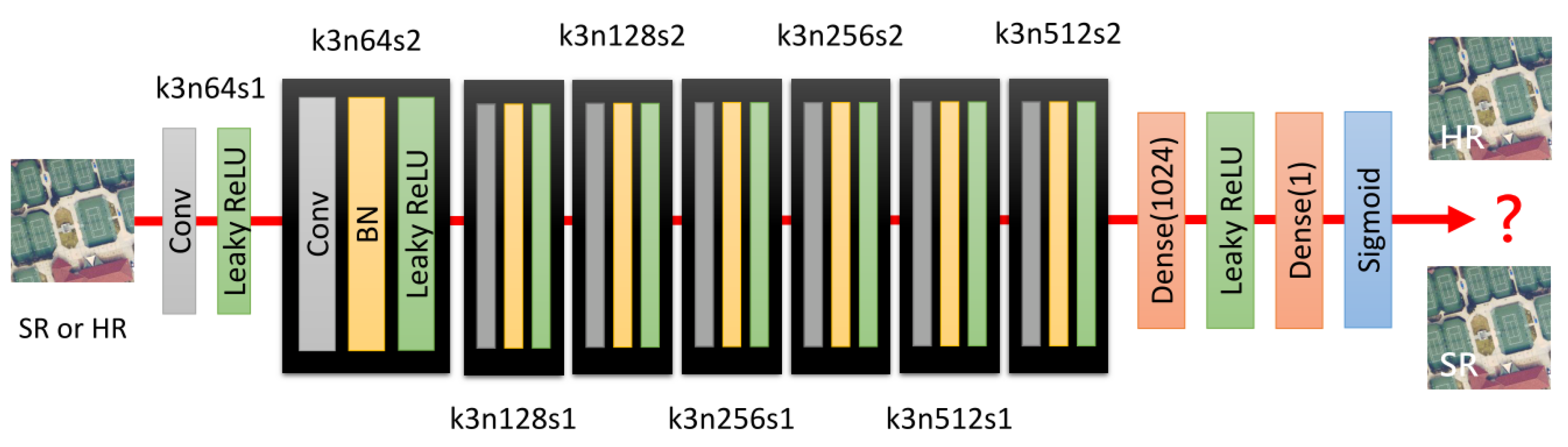
The standard GAN is used to calculate the probability whether the image is true or fake. To be able to distinguish which images are real and which are generated, we trained a discriminator network. The architecture of the discriminator is depicted in Figure 6, which contains eight convolutional layers. A batch normalization (BN) layer follows all convolutional layers, except for the first convolutional layer. Like the VGG network, the number of channels of the convolutional layer doubles from 64 to 128, and then 128 to 256, and finally 256 to 512. The stride size of the first, third, fifth, and seventh convolutional layers is set to 2, while the stride size of the remaining convolutional layers is set to 1. Moreover, the stride convolution and LeakyReLU activation () function are used rather than the maximum pooling layer. The main advantage of using stride convolution is to reduce the size of features. At the end of the network, two dense layers and a sigmoid activation function are followed to calculate the probability that the image is authentic.
4. Results and Discussions
We compare the proposed method with several satellite image SR methods based on the GAN, including SRGAN [3], ESRGAN [4], EEGAN [5], and EESRGAN [6], respectively. The test was performed on a number of popular and publicly available satellite image databases. We adopted three popular and well-known full-reference objective evaluation metrics [35,36] (i.e., peak signal-to-noise ratio (PSNR), structural similarity (SSIM) [37] and feature similarity (FSIM) [38]) to test the performance of all compared models. We also use no-reference evaluation indicators, including average gradient (AG) [39] and naturalness image quality evaluator (NIQE) [40] to evaluate those reconstructed images without high-resolution images as reference.
4.1. Databases and Experimental Parameter Setting
In this work, we use three different satellite data sets, namely, Kaggle open source dataset [41], AID [42] and WHU-RS19 [43]. For the Kaggle open source dataset, it has 1720 satellite images with size of 3099 × 2329 pixels. First of all, in the training stage, we crop images into 720 × 720 patches to increase the amount of data. Then the input LR image has a size of 180 × 180, which is obtained by down-sampling HR images using the MATLAB bicubic kernel function, which follows most existing satellite image super-resolution methods [6,19] (i.e., using a simple down-sampling model with a fixed kernel to create training images). In total, the dataset has 20,640 images.
Regarding the AID dataset [42], it contains 10,000 images in total with size of 600 × 600 and consists of 30 scene types. In addition, for the training stage of above two data sets, 80% of samples are chosen as the training set and the rest 20% of samples are treated as the test set, where the training set is divided into 90% for training and 10% for validation.
For the WHU-RS19 dataset [43], the image size of this dataset is 600 × 600, which contains a total of 1005 satellite images of 19 categories. In this dataset, we use all the images as the test data and the test model is trained on the Kaggle open source dataset.
Moreover, in order to prove that the method we proposed is effective in real scenarios, we will conduct experiments for the data set collected by SpaceWill [44]. Here we directly input the LR test image into the network trained with Kaggle, where eight scenes were selected as test samples, including the Petronas Twin Towers in Malaysia, the Pentagon Tower in the United States, the Forbidden City in Beijing, the Dubai Tower, the Beijing Olympic Pavilion, the Hong Kong Convention Center, the Saifuding Mosque in Brunei, and the Potala Palace in Qinghai-Tibet. For convenience, we cropped them into a uniform size of 1000 × 1000 pixels for testing.
For all conducted experiments, the Adam optimizer is used in the training process and we set the parameter to be 0.9. We also set the initial learning rate to be . The generator and discriminator are trained alternately until our model converges.
4.2. Comparisons with State-of-the-Art Methods in Kaggle Dataset
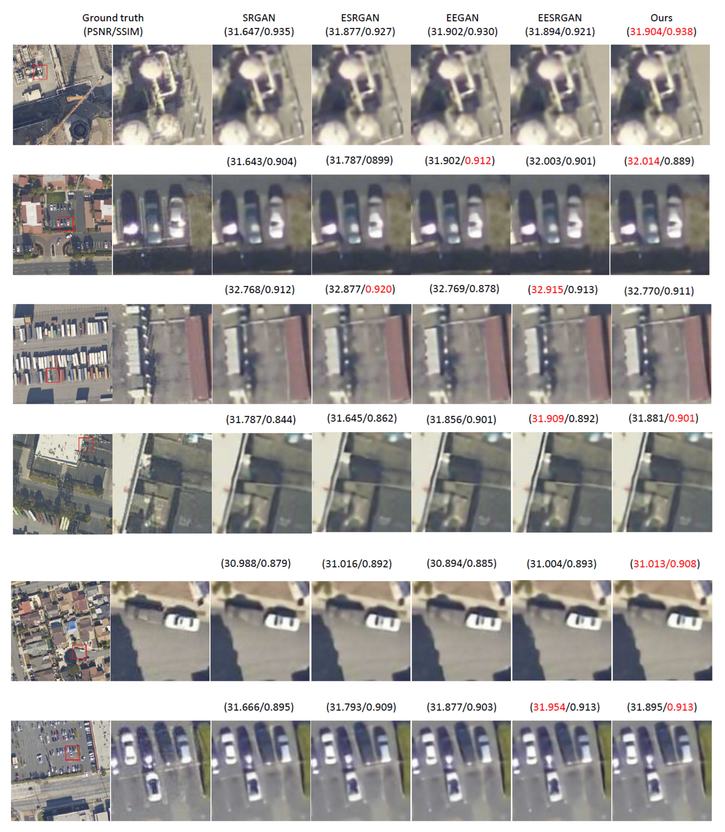
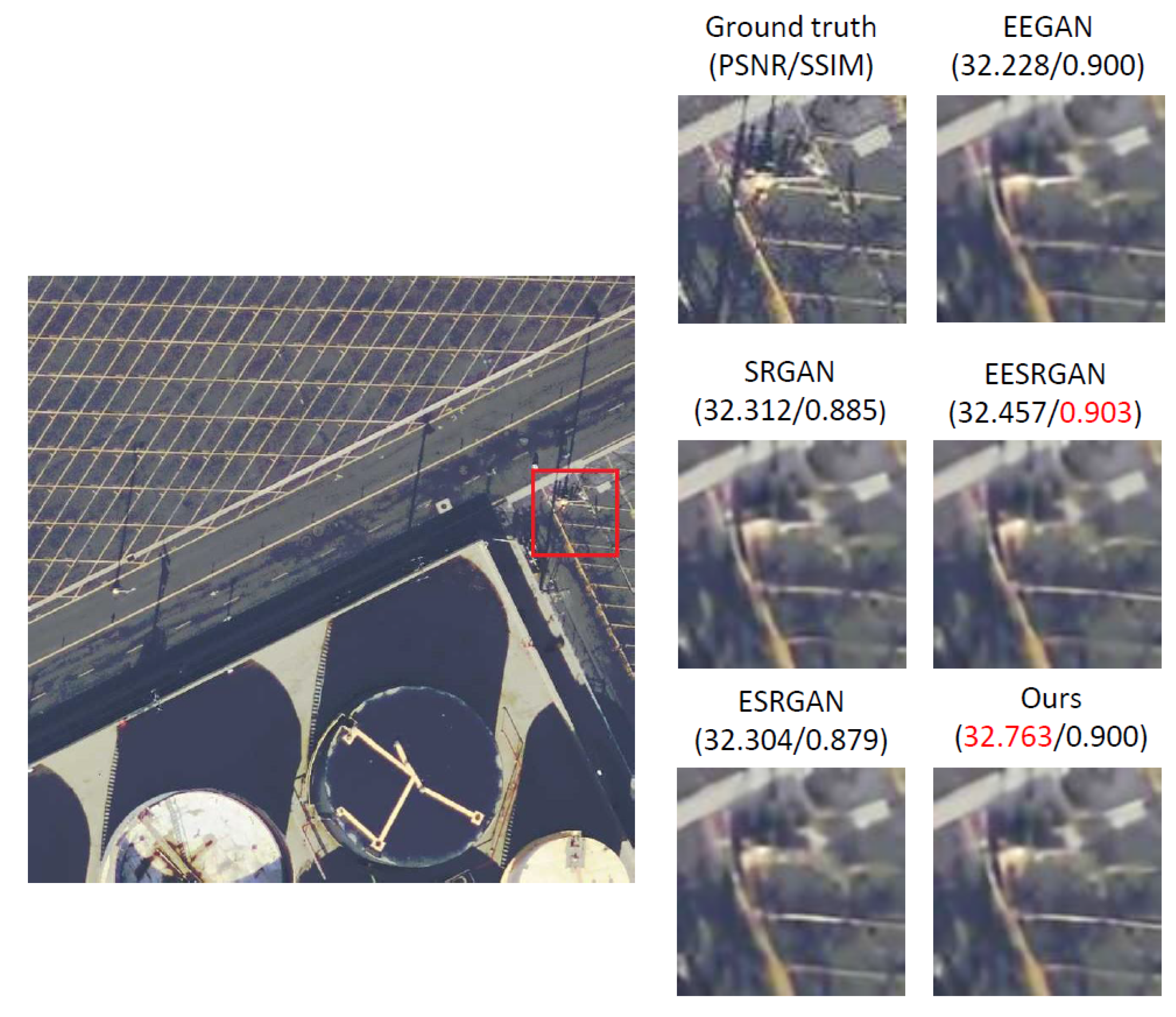
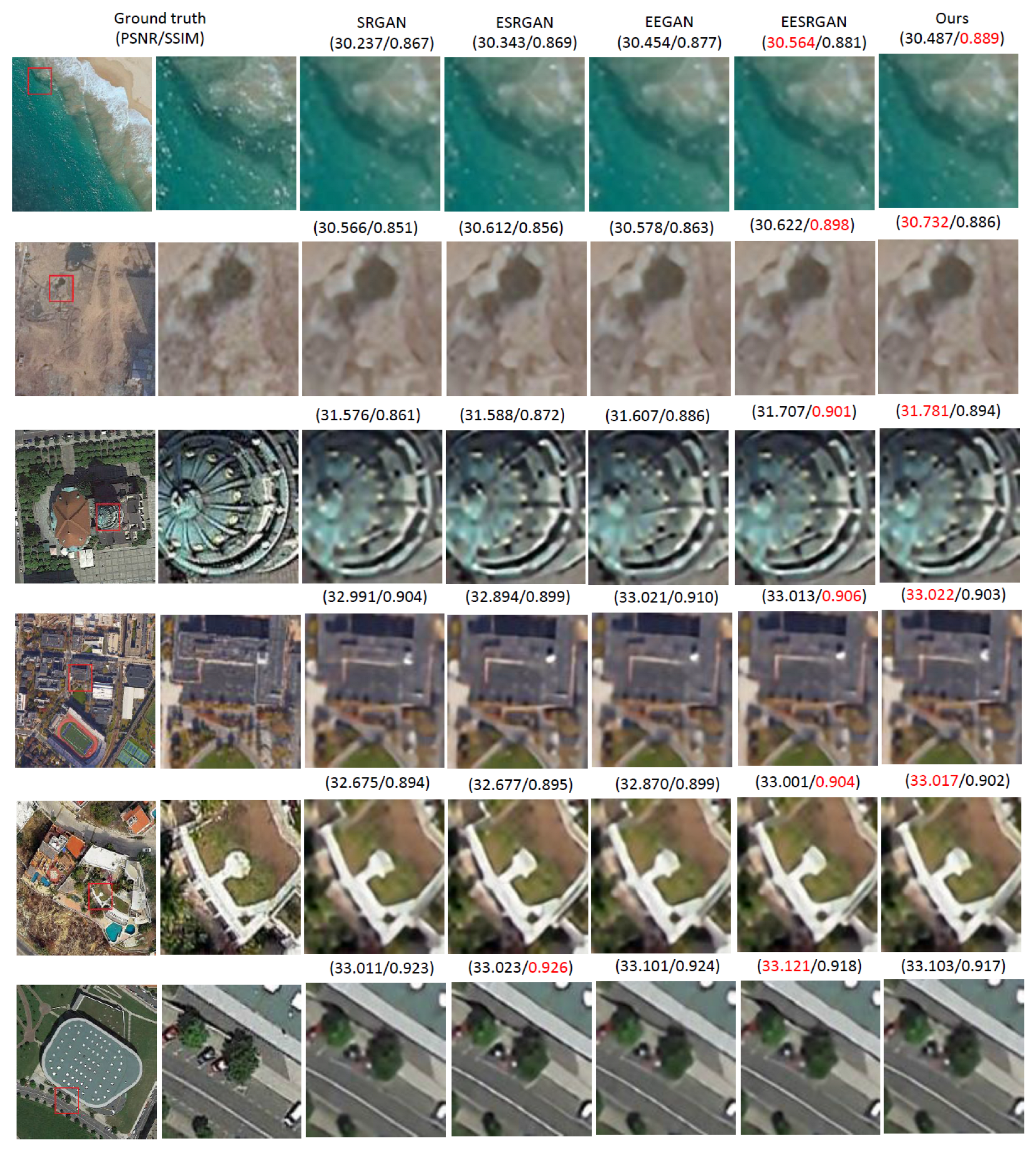
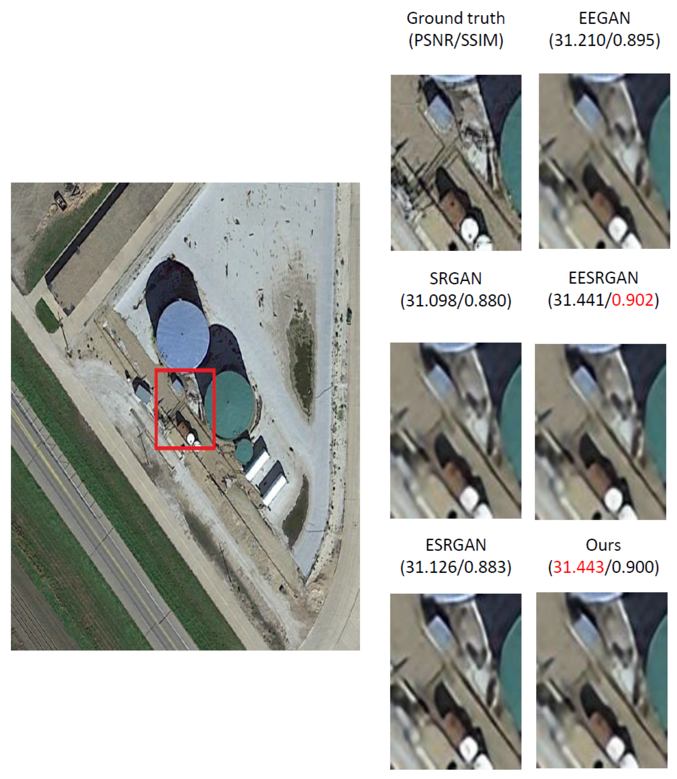
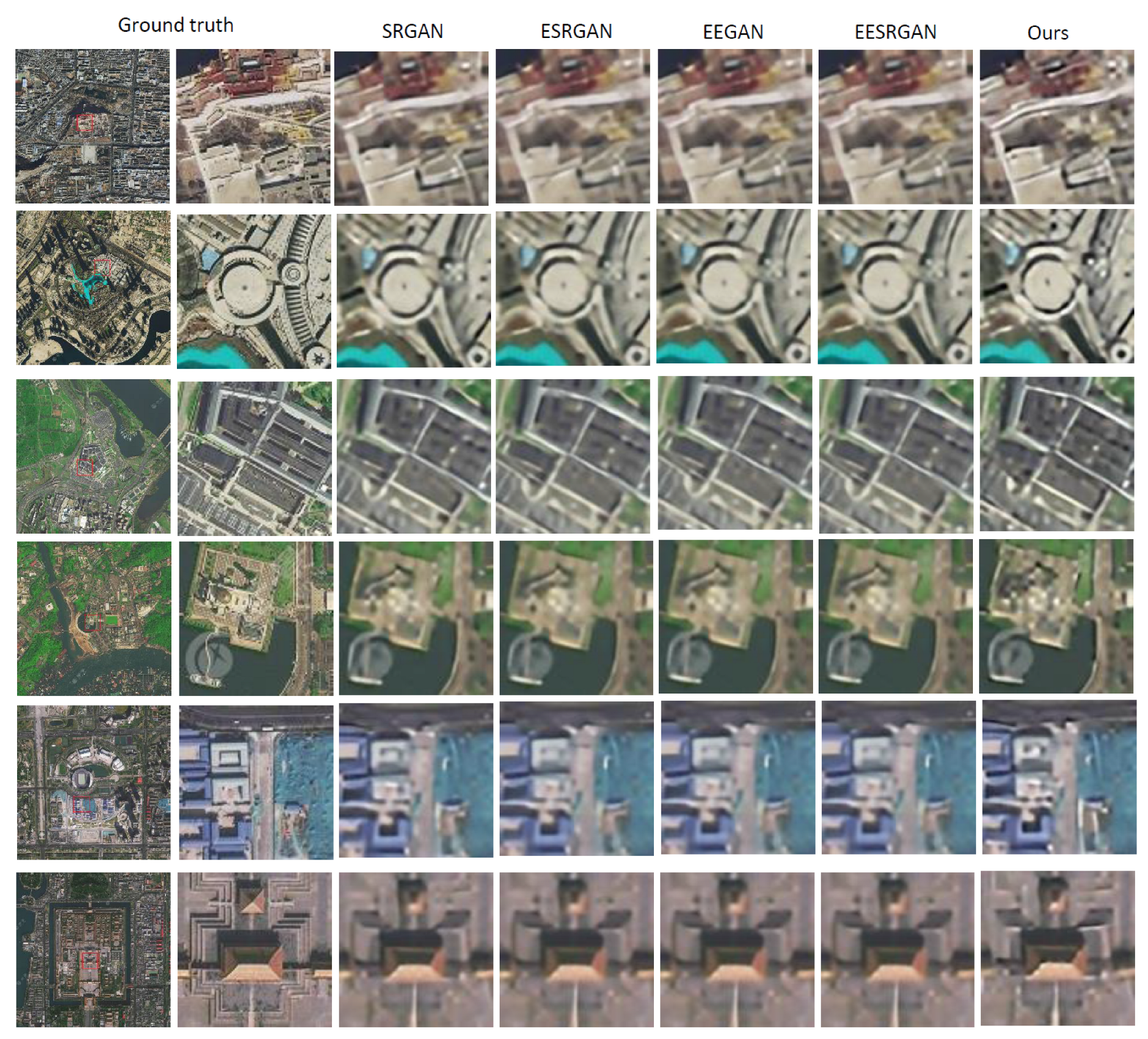
To prove the practicality of our method, we compare the proposed approach with several GAN-based SR models, including SRGAN [3], ESRGAN [4], EEGAN [5], and EESRGAN [6]. In order to have a fair comparison, we retrain these models using the same dataset. As shown in Table 5, the proposed approach has the highest scores for all the performance indices in the Kaggle dataset, including PSNR, SSIM and FSIM. Moreover, in Figure 7, it shows the SR images generated by our approach are more realistic and competitive compared with other models. Figure 8 is an enlarged partial view of the SR result of each method in the Kaggle dataset.
4.3. Comparisons with State-of-the-Art Methods in the AID Dataset
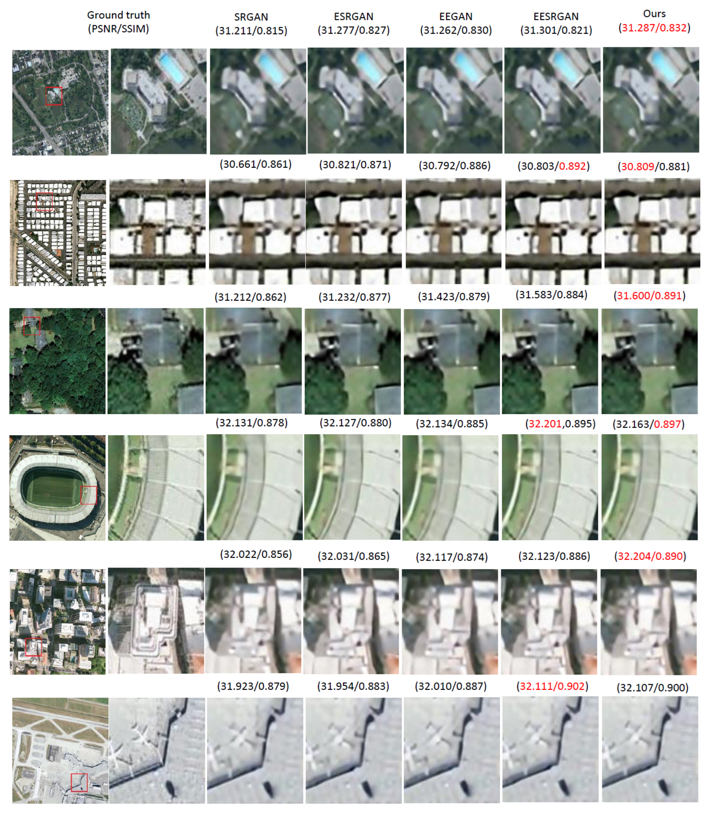
We also compare our proposed approach with other well-performed models in the AID dataset. As shown in Table 6, the proposed model still has very good scores among three performance indices, including PSNR and SSIM. Figure 9 shows the visual SR results for all compared models. Figure 10 is an enlarged partial view of the SR result of each compared method in the AID dataset.
4.4. Comparisons with State-of-the-Art Methods in the WHU-RS19 Dataset
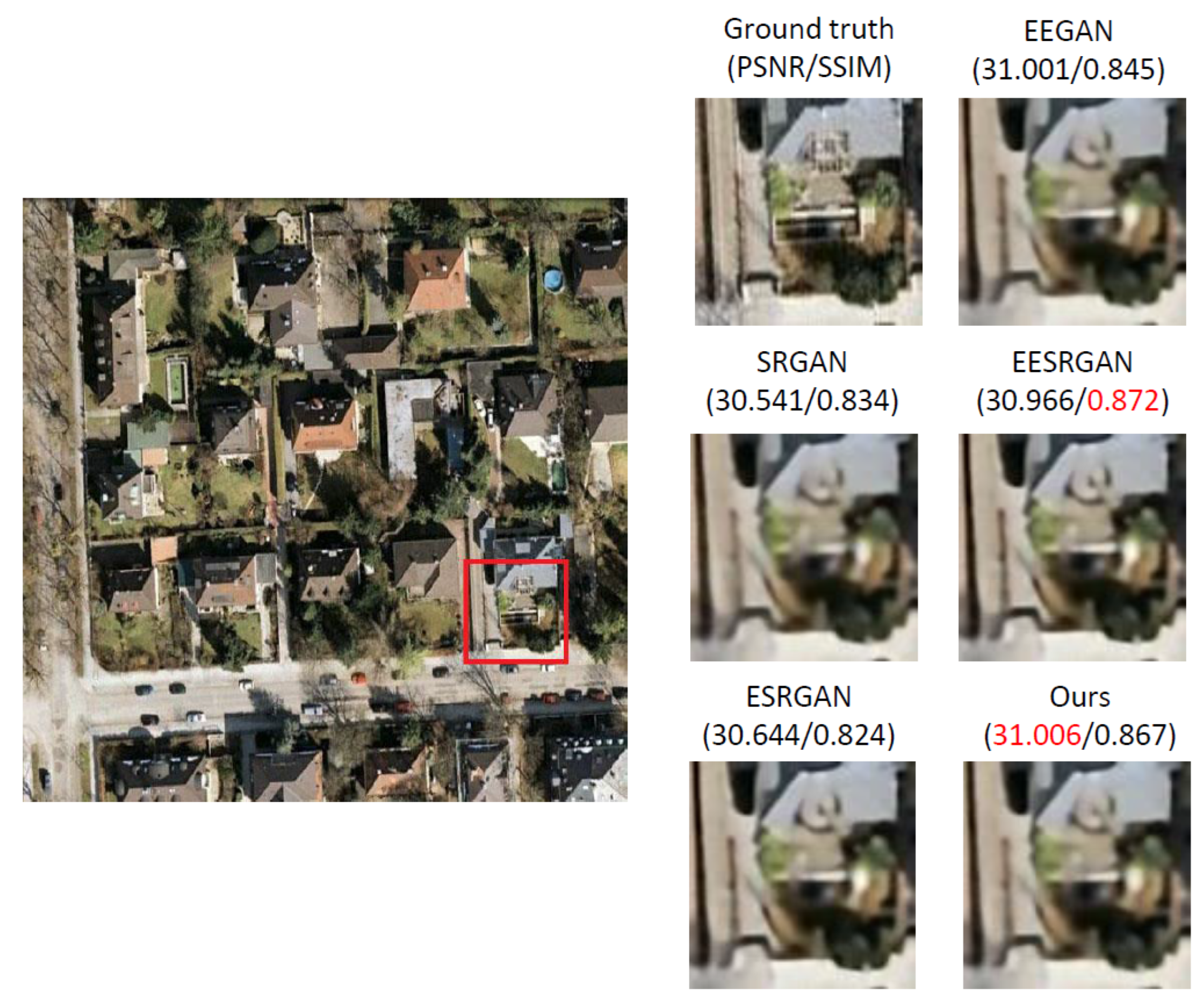
Considering that the amount of data in this data set is small, we use all the images in the dataset as a test set. For our approach and other compared SR models, we all use the model that has been trained with the Kaggle dataset to do the test. The result is shown in Table 7. Our proposed approach still has the best scores in PSNR and SSIM, except FSIM. Figure 11 shows the output SR result and Figure 12 is an enlarged partial view of the SR result of each method in the WHU-RS19 dataset. It can be observed that our approach has the best visual results compared with the other four models.
4.5. Comparisons with State-of-the-Art Methods in the SpaceWill Dataset
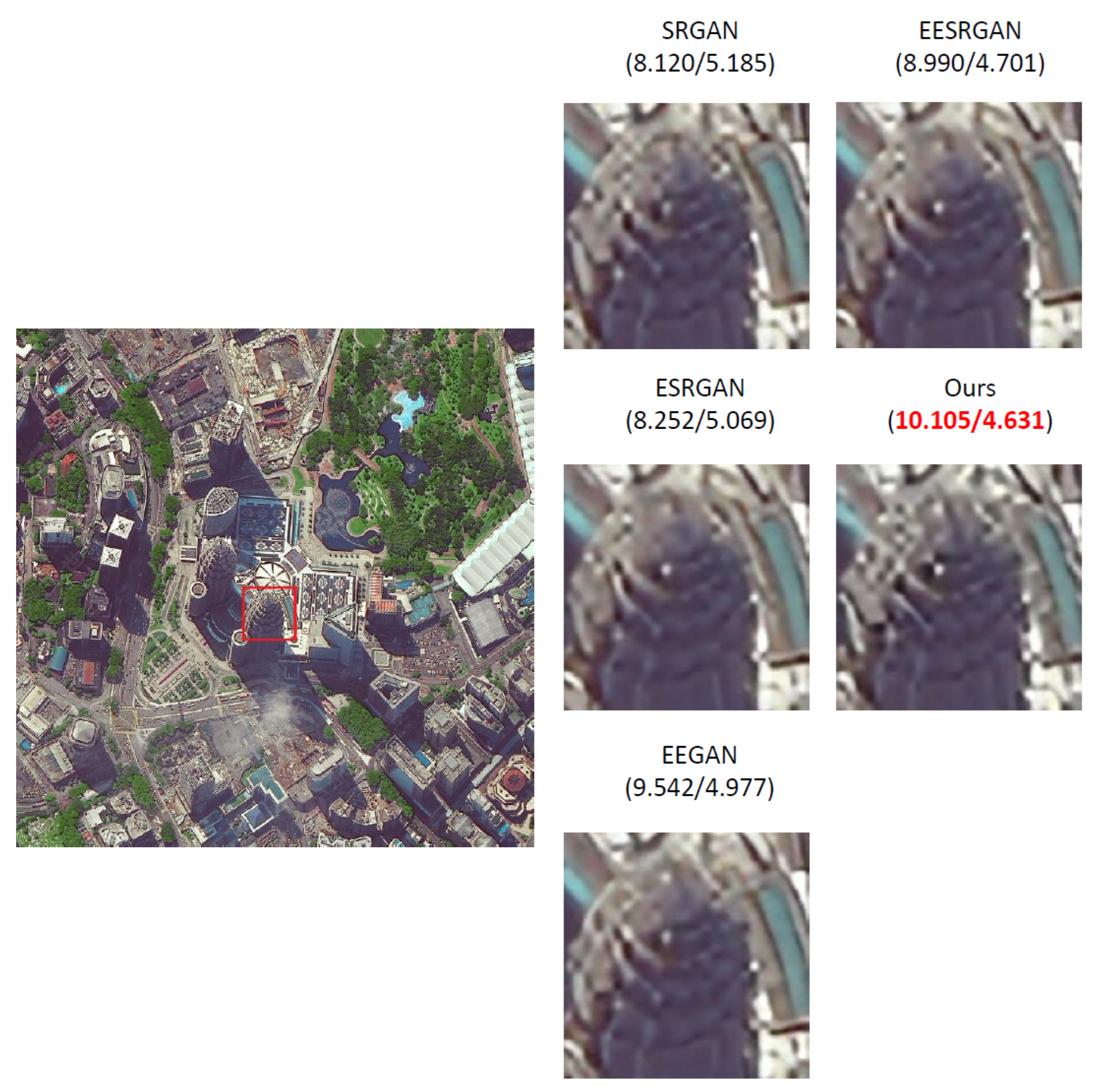
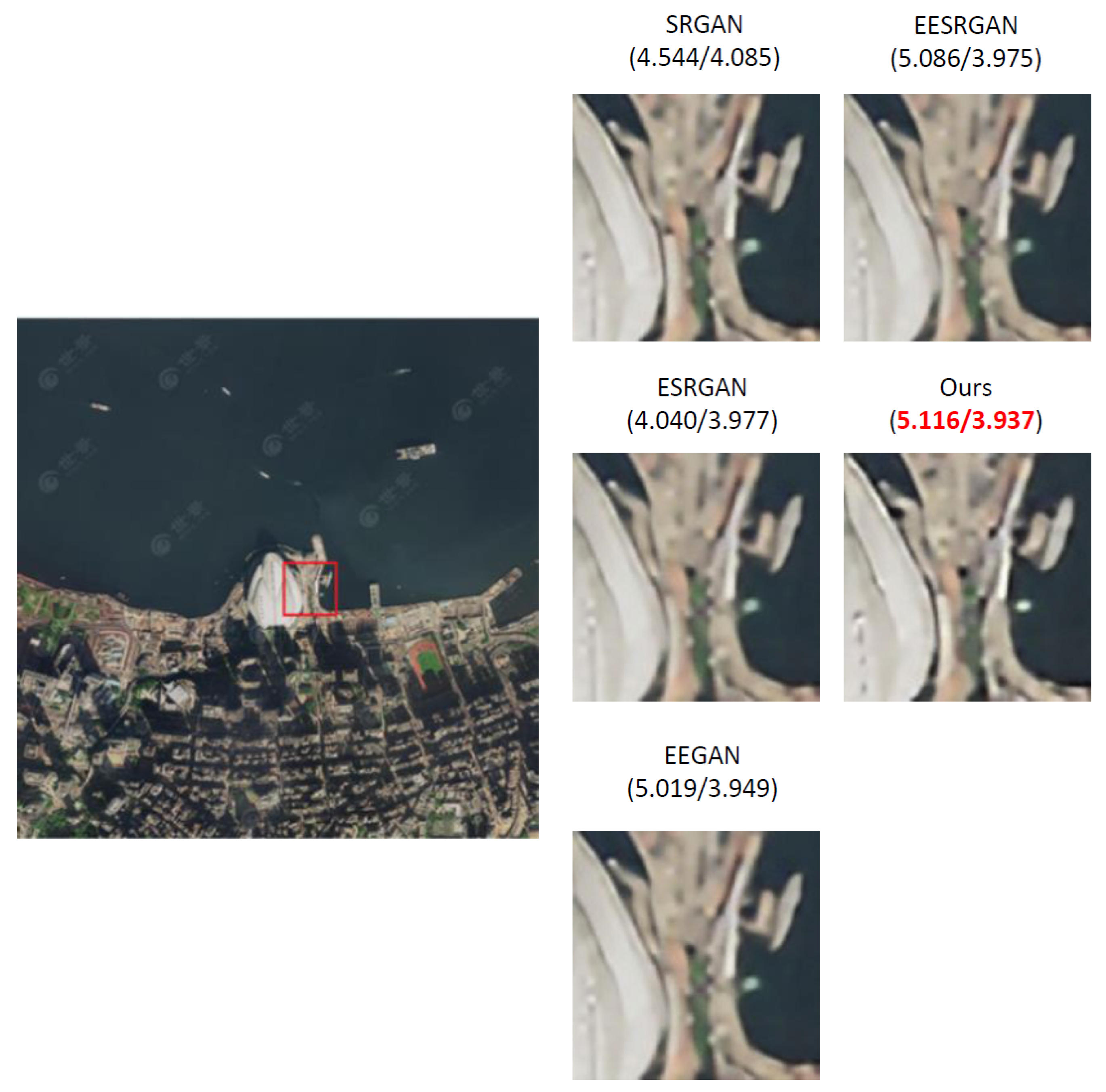
We will use the AG and NIQE to evaluate the SR results of all compared models in the SpaceWill dataset. The AG refers to the obvious difference in the grayscale near the shadow or both sides of the border of the image (i.e., the grayscale change rate). Moreover, the size of this change rate can be used to express the sharpness of the image. The larger the AG, the more layers and the clearer the image. NIQE is based on constructing a series of features used to measure image quality, and fitting these features into a multivariate Gaussian model. The larger the values of these parameters, the greater value of the NIQE and the worse of the image quality. As shown in Table 8, our approach is better than other methods. Figure 13 shows the output SR results. Figure 14 and Figure 15 are enlarged partial views of the SR results of each method in the SpaceWill dataset.
5. Conclusions
In this work, we combine the RRDB and the CNN with 2D topology to build a model with dense and complex connections. In the generator sub-network, we are able to generate SR images more close to the ground truth. Also, better and clearer features from edge can be obtained in the EESN. Moreover, the original Laplacian edge-feature extraction method has been replaced by the Canny algorithm. We also incorporate different loss functions to enhance the visual quality of the resultant SR image. By doing extensive experiments on four open databases, the proposed SR approach can generate images with better visual quality [45,46]. Based on the results of objective evaluation [47,48], our approach is indeed superior than the current SR models on satellite images. In the future, we can improve and optimize some parts of this model. For example, using different pretrained networks to extract features and compute the perceptual loss to improve the SR images. We also can try to use different identification methods or add the salient region method, which have shown good output SR results in other works. In addition, the discriminator network can be modified to have better judgments to decide whether the output image is true or fake.
Author Contributions
Conceptualization, Y.-Z.C. and T.-J.L.; methodology, Y.-Z.C.; software, Y.-Z.C.; validation, Y.-Z.C. and T.-J.L.; formal analysis, Y.-Z.C.; investigation, Y.-Z.C. and T.-J.L.; resources, Y.-Z.C. and T.-J.L.; data curation, Y.-Z.C.; writing—original draft preparation, Y.-Z.C. and T.-J.L.; writing—review and editing, T.-J.L.; visualization, Y.-Z.C.; supervision, T.-J.L. All authors have read and agreed to the published version of the manuscript.
Funding
This research received no external funding.
Institutional Review Board Statement
Not applicable.
Informed Consent Statement
Not applicable.
Data Availability Statement
Not applicable.
Conflicts of Interest
The authors declare no conflict of interest.
References
- Chang, K.C.; Liu, T.J.; Liu, K.H.; Chao, D.Y. Locating Waterfowl Farms from Satellite Images with Parallel Residual U-Net Architecture. In Proceedings of the 2020 IEEE International Conference on Systems, Man, and Cybernetics (SMC), Toronto, ON, Canada, 11–14 October 2020; pp. 114–119. [Google Scholar]
- Goodfellow, I.; Pouget-Abadie, J.; Mirza, M.; Xu, B.; Warde-Farley, D.; Ozair, S.; Courville, A.; Bengio, Y. Generative adversarial nets. Adv. Neural Inf. Process. Syst. 2014, 27, 2672–2680. [Google Scholar]
- Ledig, C.; Theis, L.; Huszár, F.; Caballero, J.; Cunningham, A.; Acosta, A.; Aitken, A.; Tejani, A.; Totz, J.; Wang, Z.; et al. Photo-realistic single image super-resolution using a generative adversarial network. In Proceedings of the IEEE Conference on Computer Vision and Pattern Recognition, Honolulu, HI, USA, 21–26 July 2017; pp. 4681–4690. [Google Scholar]
- Wang, X.; Yu, K.; Wu, S.; Gu, J.; Liu, Y.; Dong, C.; Qiao, Y.; Change Loy, C. Esrgan: Enhanced super-resolution generative adversarial networks. In Proceedings of the European Conference on Computer Vision (ECCV) Workshops, Munich, Germany, 8–14 September 2018. [Google Scholar]
- Jiang, K.; Wang, Z.; Yi, P.; Wang, G.; Lu, T.; Jiang, J. Edge-enhanced GAN for remote sensing image superresolution. IEEE Trans. Geosci. Remote Sens. 2019, 57, 5799–5812. [Google Scholar] [CrossRef]
- Rabbi, J.; Ray, N.; Schubert, M.; Chowdhury, S.; Chao, D. Small-object detection in remote sensing images with end-to-end edge-enhanced GAN and object detector network. Remote Sens. 2020, 12, 1432. [Google Scholar] [CrossRef]
- Simonyan, K.; Zisserman, A. Very deep convolutional networks for large-scale image recognition. arXiv 2014, arXiv:1409.1556. [Google Scholar]
- Canny, J. A computational approach to edge detection. IEEE Trans. Pattern Anal. Mach. Intell. 1986, 6, 679–698. [Google Scholar] [CrossRef]
- Chen, Y.Z.; Liu, T.J.; Liu, K.H. Super-Resolution of Satellite Images by two-Dimensional RRDB and Edge-Enhancement Generative Adversarial Network. In Proceedings of the ICASSP 2022–2022 IEEE International Conference on Acoustics, Speech and Signal Processing (ICASSP), Singapore, 7–13 May 2022; pp. 1825–1829. [Google Scholar]
- Lai, W.S.; Huang, J.B.; Ahuja, N.; Yang, M.H. Deep laplacian pyramid networks for fast and accurate super-resolution. In Proceedings of the IEEE Conference on Computer Vision and Pattern Recognition, Honolulu, HI, USA, 21–26 July 2017; pp. 624–632. [Google Scholar]
- Tai, Y.; Yang, J.; Liu, X. Image super-resolution via deep recursive residual network. In Proceedings of the IEEE Conference on Computer Vision and Pattern Recognition, Honolulu, HI, USA, 21–26 July 2017; pp. 3147–3155. [Google Scholar]
- Lim, B.; Son, S.; Kim, H.; Nah, S.; Mu Lee, K. Enhanced deep residual networks for single image super-resolution. In Proceedings of the IEEE Conference on Computer Vision and Pattern Recognition Workshops, Honolulu, HI, USA, 21–26 July 2017; pp. 136–144. [Google Scholar]
- Zhou, L.; Wang, Z.; Luo, Y.; Xiong, Z. Separability and compactness network for image recognition and superresolution. IEEE Trans. Neural Netw. Learn. Syst. 2019, 30, 3275–3286. [Google Scholar] [CrossRef]
- Zuo, C.; Qian, J.; Feng, S.; Yin, W.; Li, Y.; Fan, P.; Han, J.; Qian, K.; Chen, Q. Deep learning in optical metrology: A review. Light. Sci. Appl. 2022, 11, 1–54. [Google Scholar] [CrossRef]
- Dong, C.; Loy, C.C.; He, K.; Tang, X. Image super-resolution using deep convolutional networks. IEEE Trans. Pattern Anal. Mach. Intell. 2015, 38, 295–307. [Google Scholar] [CrossRef] [Green Version]
- Shi, W.; Caballero, J.; Huszár, F.; Totz, J.; Aitken, A.P.; Bishop, R.; Rueckert, D.; Wang, Z. Real-time single image and video super-resolution using an efficient sub-pixel convolutional neural network. In Proceedings of the IEEE Conference on Computer Vision and Pattern Recognition, Las Vegas, NV, USA, 27–30 June 2016; pp. 1874–1883. [Google Scholar]
- He, K.; Zhang, X.; Ren, S.; Sun, J. Deep residual learning for image recognition. In Proceedings of the IEEE Conference on Computer Vision and Pattern Recognition, Las Vegas, NV, USA, 27–30 June 2016; pp. 770–778. [Google Scholar]
- Kawulok, M.; Piechaczek, S.; Hrynczenko, K.; Benecki, P.; Kostrzewa, D.; Nalepa, J. On training deep networks for satellite image super-resolution. In Proceedings of the IGARSS 2019-2019 IEEE International Geoscience and Remote Sensing Symposium, Yokohama, Japan, 28 July–2 August 2019; pp. 3125–3128. [Google Scholar]
- Shermeyer, J.; Van Etten, A. The effects of super-resolution on object detection performance in satellite imagery. In Proceedings of the IEEE/CVF Conference on Computer Vision and Pattern Recognition Workshops, Long Beach, CA, USA, 16–17 July 2019. [Google Scholar]
- Wei, Z.; Liu, Y. Satellite Image Small Target Application Based on Deep Segmented Residual Neural Network. In Proceedings of the 2020 IEEE International Conference on Mechatronics and Automation (ICMA), Beijing, China, 13–16 October 2020; pp. 100–104. [Google Scholar]
- Rout, L.; Shah, S.; Moorthi, S.M.; Dhar, D. Monte-Carlo Siamese policy on actor for satellite image super resolution. In Proceedings of the IEEE/CVF Conference on Computer Vision and Pattern Recognition Workshops, Seattle, WA, USA, 14–19 June 2020; pp. 194–195. [Google Scholar]
- Zhu, X.; Talebi, H.; Shi, X.; Yang, F.; Milanfar, P. Super-resolving commercial satellite imagery using realistic training data. In Proceedings of the 2020 IEEE International Conference on Image Processing (ICIP), Abu Dhabi, United Arab Emirates, 25–28 October 2020; pp. 498–502. [Google Scholar]
- Müller, M.U.; Ekhtiari, N.; Almeida, R.M.; Rieke, C. Super-resolution of multispectral satellite images using convolutional neural networks. arXiv 2020, arXiv:2002.00580. [Google Scholar] [CrossRef]
- Wang, J.; Gao, K.; Zhang, Z.; Ni, C.; Hu, Z.; Chen, D.; Wu, Q. Multisensor remote sensing imagery super-resolution with conditional GAN. J. Remote Sens. 2021, 2021, 1–11. [Google Scholar] [CrossRef]
- Tewari, A.; Prateek, C.; Khanna, N. In-orbit lunar satellite image super resolution for selective data transmission. arXiv 2021, arXiv:2110.10109. [Google Scholar]
- Zhu, X.; Zhang, L.; Zhang, L.; Liu, X.; Shen, Y.; Zhao, S. Generative adversarial network-based image super-resolution with a novel quality loss. In Proceedings of the 2019 International Symposium on Intelligent Signal Processing and Communication Systems (ISPACS), Taipei, Taiwan, 3–6 December 2019; pp. 1–2. [Google Scholar]
- Gonzalez, R.C.; Woods, R.E. Digital Image Processing, 3rd ed.; Cliffs, E., Ed.; Prentice-Hall: Englewood Cliffs, NJ, USA, 2007. [Google Scholar]
- Pratt, W.K. Digital Image Processing, 4th ed.; Wiley: New York, NY, USA, 2007. [Google Scholar]
- Liu, T.J.; Lin, W.; Kuo, C.C.J. Image quality assessment using multi-method fusion. IEEE Trans. Image Process. 2012, 22, 1793–1807. [Google Scholar] [CrossRef] [PubMed]
- Liu, T.J.; Liu, K.H.; Lin, J.Y.; Lin, W.; Kuo, C.C.J. A paraboost method to image quality assessment. IEEE Trans. Neural Netw. Learn. Syst. 2015, 28, 107–121. [Google Scholar] [CrossRef] [PubMed]
- Liu, T.J.; Liu, K.H. No-reference image quality assessment by wide-perceptual-domain scorer ensemble method. IEEE Trans. Image Process. 2017, 27, 1138–1151. [Google Scholar] [CrossRef] [PubMed]
- Wen, K.Y.; Liu, T.J.; Liu, K.H.; Chao, D.Y. Identifying Poultry Farms from Satellite Images with Residual Dense U-Net. In Proceedings of the 2020 IEEE International Conference on Systems, Man, and Cybernetics (SMC), Toronto, ON, Canada, 11–14 October 2020; pp. 102–107. [Google Scholar]
- Shrivakshan, G.; Chandrasekar, C. A comparison of various edge detection techniques used in image processing. Int. J. Comput. Sci. Issues (IJCSI) 2012, 9, 269. [Google Scholar]
- Johnson, J.; Alahi, A.; Fei-Fei, L. Perceptual losses for real-time style transfer and super-resolution. In Proceedings of the European Conference on Computer Vision, Amsterdam, The Netherlands, 11–14 October 2016; Springer: Berlin/Heidelberg, Germany, 2016; pp. 694–711. [Google Scholar]
- Liu, T.J.; Liu, H.H.; Pei, S.C.; Liu, K.H. A high-definition diversity-scene database for image quality assessment. IEEE Access 2018, 6, 45427–45438. [Google Scholar] [CrossRef]
- Liu, T.J. Study of visual quality assessment on pattern images: Subjective evaluation and visual saliency effects. IEEE Access 2018, 6, 61432–61444. [Google Scholar] [CrossRef]
- Wang, Z.; Bovik, A.C.; Sheikh, H.R.; Simoncelli, E.P. Image quality assessment: From error visibility to structural similarity. IEEE Trans. Image Process. 2004, 13, 600–612. [Google Scholar] [CrossRef] [Green Version]
- Zhang, L.; Zhang, L.; Mou, X.; Zhang, D. FSIM: A feature similarity index for image quality assessment. IEEE Trans. Image Process. 2011, 20, 2378–2386. [Google Scholar] [CrossRef] [Green Version]
- Chen, A.A.; Chai, X.; Chen, B.; Bian, R.; Chen, Q. A novel stochastic stratified average gradient method: Convergence rate and its complexity. In Proceedings of the 2018 International Joint Conference on Neural Networks (IJCNN), Rio de Janeiro, Brazil, 8–13 July 2018; pp. 1–8. [Google Scholar]
- Mittal, A.; Soundararajan, R.; Bovik, A.C. Making a “completely blind” image quality analyzer. IEEE Signal Process. Lett. 2012, 20, 209–212. [Google Scholar] [CrossRef]
- Kaggle Open Source Data Set. [Online]. 2016. Available online: https://www.kaggle.com/c/draper-satellite-image-chronology/data (accessed on 8 November 2022).
- Xia, G.S.; Hu, J.; Hu, F.; Shi, B.; Bai, X.; Zhong, Y.; Zhang, L.; Lu, X. AID: A benchmark data set for performance evaluation of aerial scene classification. IEEE Trans. Geosci. Remote Sens. 2017, 55, 3965–3981. [Google Scholar] [CrossRef] [Green Version]
- Xia, G.S.; Yang, W.; Delon, J.; Gousseau, Y.; Sun, H.; Maître, H. Structural high-resolution satellite image indexing. In Proceedings of the ISPRS TC VII Symposium-100 Years ISPRS, Vienna, Austria, 5–7 July 2010; Volume 38, pp. 298–303. [Google Scholar]
- SpaceWill SuperView-1 Data Set. [Online]. 2018. Available online: http://www.spacewillinfo.com/superview-1/index.html#pos03 (accessed on 9 November 2020).
- Liu, T.J.; Lin, W.; Kuo, C.C.J. Recent developments and future trends in visual quality assessment. In Proceedings of the Asia-Pacific Signal Information Processing Association Annual Summit and Conference (APSIPA ASC), Xi’an, China, 18–21 October 2011; pp. 1–10. [Google Scholar]
- Liu, T.J.; Liu, K.H.; Shen, K.H. Learning based no-reference metric for assessing quality of experience of stereoscopic images. J. Vis. Commun. Image Represent. 2019, 61, 272–283. [Google Scholar] [CrossRef]
- Chen, B.X.; Liu, T.J.; Liu, K.H.; Liu, H.H.; Pei, S.C. Image super-resolution using complex dense block on generative adversarial networks. In Proceedings of the 2019 IEEE International Conference on Image Processing (ICIP), Taipei, Taiwan, 22–25 September 2019; pp. 2866–2870. [Google Scholar]
- Su, Y.Z.; Liu, T.J.; Liu, K.H.; Liu, H.H.; Pei, S.C. Image inpainting for random areas using dense context features. In Proceedings of the 2019 IEEE International Conference on Image Processing (ICIP), Taipei, Taiwan, 22–25 September 2019; pp. 4679–4683. [Google Scholar]
Figure 1.
Proposed network architecture.

Figure 2.
Proposed generator architecture.

Figure 3.
The convolutional layers with 2D topology.

Figure 4.
The RDB in the RRDB connection has two-dimensional topological convolution layers.

Figure 5.
Edge extraction and enhancement, where Edge* represents the image after edge enhancement.

Figure 6.
Network architecture of the discriminator.

Figure 7.
SR visual result comparison for all models in the Kaggle dataset, where the best results are shown in red font.
Figure 7.
SR visual result comparison for all models in the Kaggle dataset, where the best results are shown in red font.

Figure 8.
An enlarged partial view of the SR result of each method in the Kaggle dataset, where the best results are shown in red font.
Figure 8.
An enlarged partial view of the SR result of each method in the Kaggle dataset, where the best results are shown in red font.

Figure 9.
SR visual result comparison for all models in the AID dataset, where the best results are shown in red font.
Figure 9.
SR visual result comparison for all models in the AID dataset, where the best results are shown in red font.

Figure 10.
An enlarged partial view of the SR result of each method in the AID dataset, where the best results are shown in red font.
Figure 10.
An enlarged partial view of the SR result of each method in the AID dataset, where the best results are shown in red font.

Figure 11.
SR visual result comparison for all models in the WHU-RS19 dataset, where the best results are shown in red font.
Figure 11.
SR visual result comparison for all models in the WHU-RS19 dataset, where the best results are shown in red font.

Figure 12.
An enlarged partial view of the SR result of each method in the WHU-RS19 dataset, where the best results are shown in red font.
Figure 12.
An enlarged partial view of the SR result of each method in the WHU-RS19 dataset, where the best results are shown in red font.

Figure 13.
SR visual result comparison for all models in the SpaceWill dataset.

Figure 14.
An enlarged partial view of the SR result of each method in the SpaceWill dataset—sample image 1, where the best results are shown in red font.
Figure 14.
An enlarged partial view of the SR result of each method in the SpaceWill dataset—sample image 1, where the best results are shown in red font.

Figure 15.
An enlarged partial view of the SR result of each method in the SpaceWill dataset—sample image 2, where the best results are shown in red font.
Figure 15.
An enlarged partial view of the SR result of each method in the SpaceWill dataset—sample image 2, where the best results are shown in red font.


Table 1.
The best results of four combinations used to replace the original block in the UDSN, where the best results are shown in boldface.
Table 1.
The best results of four combinations used to replace the original block in the UDSN, where the best results are shown in boldface.
| Block Type | Topology | # of Blocks | # of Conv. Layers | PSNR | SSIM | FSIM |
|---|---|---|---|---|---|---|
| RDB | 1D | 7 | 3 | 31.401 | 0.845 | 0.985 |
| RDB | 2D | 6 | 4 | 32.560 | 0.901 | 0.990 |
| RRDB | 1D | 4 | 5 | 32.074 | 0.882 | 0.985 |
| RRDB | 2D | 3 | 5 | 32.774 | 0.899 | 0.991 |
Table 2.
The best results of four combinations used to replace the original block in the EESN, where the best results are shown in boldface.
Table 2.
The best results of four combinations used to replace the original block in the EESN, where the best results are shown in boldface.
| Block Type | Topology | # of Blocks | # of Conv. Layers | PSNR | SSIM | FSIM |
|---|---|---|---|---|---|---|
| RDB | 1D | 3 | 3 | 32.755 | 0.903 | 0.990 |
| RDB | 2D | 3 | 2 | 32.676 | 0.890 | 0.986 |
| RRDB | 1D | 3 | 2 | 32.935 | 0.910 | 0.989 |
| RRDB | 2D | 2 | 3 | 32.947 | 0.913 | 0.990 |
Table 3.
Comparison of edge-extraction methods, where the best results are shown in boldface.
| Edge-Extraction Method | PSNR | SSIM | FSIM |
|---|---|---|---|
| Laplacian | 32.947 | 0.913 | 0.990 |
| Sobel | 32.950 | 0.906 | 0.984 |
| Canny | 33.011 | 0.918 | 0.994 |
Table 4.
Ablation experiments.
| UDSN | EESN | Edge-Extraction | PSNR | SSIM | FSIM | ||||||
|---|---|---|---|---|---|---|---|---|---|---|---|
| DB | DB | Laplacian | ✔ | ✔ | ✔ | ✗ | ✗ | ✗ | 31.843 | 0.874 | 0.988 |
| RDB | DB | Laplacian | ✔ | ✔ | ✔ | ✗ | ✗ | ✗ | 31.401 | 0.845 | 0.985 |
| 2D-RDB | DB | Laplacian | ✔ | ✔ | ✔ | ✗ | ✗ | ✗ | 32.560 | 0.901 | 0.990 |
| RRDB | DB | Laplacian | ✔ | ✔ | ✔ | ✗ | ✗ | ✗ | 32.074 | 0.882 | 0.985 |
| 2D-RRDB | DB | Laplacian | ✔ | ✔ | ✔ | ✗ | ✗ | ✗ | 32.774 | 0.899 | 0.991 |
| 2D-RRDB | RDB | Laplacian | ✔ | ✔ | ✔ | ✗ | ✗ | ✗ | 32.755 | 0.903 | 0.990 |
| 2D-RRDB | 2D-RDB | Laplacian | ✔ | ✔ | ✔ | ✗ | ✗ | ✗ | 32.676 | 0.890 | 0.986 |
| 2D-RRDB | RRDB | Laplacian | ✔ | ✔ | ✔ | ✗ | ✗ | ✗ | 32.935 | 0.910 | 0.989 |
| 2D-RRDB | 2D-RRDB | Laplacian | ✔ | ✔ | ✔ | ✗ | ✗ | ✗ | 32.947 | 0.913 | 0.990 |
| 2D-RRDB | 2D-RRDB | Sobel | ✔ | ✔ | ✔ | ✗ | ✗ | ✗ | 32.950 | 0.906 | 0.984 |
| 2D-RRDB | 2D-RRDB | Canny | ✔ | ✔ | ✔ | ✗ | ✗ | ✗ | 33.011 | 0.918 | 0.994 |
| 2D-RRDB | 2D-RRDB | Canny | ✔ | ✔ | ✔ | ✔ | ✗ | ✗ | 33.057 | 0.923 | 0.990 |
| 2D-RRDB | 2D-RRDB | Canny | ✔ | ✔ | ✔ | ✔ | ✔ | ✗ | 33.103 | 0.925 | 0.987 |
| 2D-RRDB | 2D-RRDB | Canny | ✔ | ✔ | ✔ | ✔ | ✗ | ✔ | 33.081 | 0.917 | 0.994 |
| 2D-RRDB | 2D-RRDB | Canny | ✔ | ✔ | ✔ | ✔ | ✔ | ✔ | 33.111 | 0.921 | 0.990 |
Table 5.
SR result performance comparison in the Kaggle dataset, where the best results are shown in boldface.
Table 5.
SR result performance comparison in the Kaggle dataset, where the best results are shown in boldface.
| SRGAN [3] | ESRGAN [4] | EEGAN [5] | EESRGAN [6] | Ours | |
|---|---|---|---|---|---|
| PSNR | 32.215 | 32.396 | 32.463 | 32.804 | 33.001 |
| SSIM | 0.893 | 0.887 | 0.901 | 0.899 | 0.906 |
| FSIM | 0.987 | 0.992 | 0.991 | 0.990 | 0.993 |
Table 6.
SR result performance comparison in the AID dataset, where the best results are shown in boldface.
Table 6.
SR result performance comparison in the AID dataset, where the best results are shown in boldface.
| SRGAN [3] | ESRGAN [4] | EEGAN [5] | EESRGAN [6] | Ours | |
|---|---|---|---|---|---|
| PSNR | 32.164 | 32.250 | 32.140 | 32.335 | 32.399 |
| SSIM | 0.876 | 0.883 | 0.903 | 0.896 | 0.908 |
| FSIM | 0.980 | 0.989 | 0.990 | 0.992 | 0.990 |
Table 7.
SR result performance comparison in the WHU-RS19 dataset, where the best results are shown in boldface.
Table 7.
SR result performance comparison in the WHU-RS19 dataset, where the best results are shown in boldface.
| SRGAN [3] | ESRGAN [4] | EEGAN [5] | EESRGAN [6] | Ours | |
|---|---|---|---|---|---|
| PSNR | 31.703 | 31.786 | 31.827 | 31.839 | 32.010 |
| SSIM | 0.862 | 0.855 | 0.871 | 0.844 | 0.881 |
| FSIM | 0.980 | 0.983 | 0.983 | 0.984 | 0.980 |
Table 8.
SR result performance comparison in the SpaceWill dataset, where the best results are shown in boldface.
Table 8.
SR result performance comparison in the SpaceWill dataset, where the best results are shown in boldface.
| SRGAN [3] | ESRGAN [4] | EEGAN [5] | EESRGAN [6] | Ours | ||||||
|---|---|---|---|---|---|---|---|---|---|---|
| AG | NIQE | AG | NIQE | AG | NIQE | AG | NIQE | AG | NIQE | |
| Petronas Twin Towers | 8.120 | 5.185 | 8.252 | 5.069 | 9.542 | 4.977 | 8.990 | 4.701 | 10.105 | 4.631 |
| Pentagonal Building | 5.974 | 5.010 | 5.241 | 4.921 | 5.238 | 4.333 | 6.043 | 4.076 | 6.427 | 4.301 |
| Forbidden City | 6.043 | 5.179 | 5.459 | 5.232 | 5.783 | 5.135 | 6.324 | 5.065 | 6.641 | 5.013 |
| Dubai Tower | 8.838 | 4.623 | 8.774 | 4.737 | 10.017 | 4.952 | 9.563 | 4.501 | 10.991 | 4.510 |
| Beijing Olympic Pavilion | 6.679 | 4.693 | 5.812 | 4.723 | 6.956 | 4.566 | 6.637 | 4.894 | 7.311 | 4.762 |
| Hong Kong Convention and Exhibition Center | 4.544 | 4.085 | 4.040 | 3.977 | 5.019 | 3.949 | 5.086 | 3.975 | 5.116 | 3.937 |
| Saifuding Mosque | 4.554 | 4.468 | 4.780 | 4.244 | 5.211 | 4.036 | 5.919 | 4.001 | 5.751 | 3.990 |
| Potala Palace in Qinghai-Tibet | 9.535 | 5.325 | 9.466 | 5.417 | 11.697 | 5.663 | 10.601 | 5.508 | 11.231 | 5.369 |
Publisher’s Note: MDPI stays neutral with regard to jurisdictional claims in published maps and institutional affiliations. |
© 2022 by the authors. Licensee MDPI, Basel, Switzerland. This article is an open access article distributed under the terms and conditions of the Creative Commons Attribution (CC BY) license (https://creativecommons.org/licenses/by/4.0/).
Share and Cite
MDPI and ACS Style
Liu, T.-J.; Chen, Y.-Z. Satellite Image Super-Resolution by 2D RRDB and Edge-Enhanced Generative Adversarial Network. Appl. Sci. 2022, 12, 12311. https://0-doi-org.brum.beds.ac.uk/10.3390/app122312311
AMA Style
Liu T-J, Chen Y-Z. Satellite Image Super-Resolution by 2D RRDB and Edge-Enhanced Generative Adversarial Network. Applied Sciences. 2022; 12(23):12311. https://0-doi-org.brum.beds.ac.uk/10.3390/app122312311
Chicago/Turabian StyleLiu, Tsung-Jung, and Yu-Zhang Chen. 2022. "Satellite Image Super-Resolution by 2D RRDB and Edge-Enhanced Generative Adversarial Network" Applied Sciences 12, no. 23: 12311. https://0-doi-org.brum.beds.ac.uk/10.3390/app122312311
Note that from the first issue of 2016, this journal uses article numbers instead of page numbers. See further details here.