Modeling the Submergence Depth of Oil Well States and Its Applications

Abstract

Obtaining the liquid storage state of oil wells in real time is very important for oilfield production. In this paper, under the premise of fully considering the transformation factors of full-pumping and nonfull-pumping states of oil wells, submergence depth models suitable for full- and nonfull-pumping wells are constructed. To reduce the application complexity of the models, parameter-reduction processing is performed to enhance the usability of the models. By analyzing the change trend of the submergence depth during the rising, maintaining, and falling of the oil well in the full-pumping state and nonfull-pumping state models, the judgment criteria for the transition of the oil well state are provided. On this basis, the application methods of nonlinear interpolation and least squares curve-fitting numerical solutions of submergence depth models are studied, and the unique existence of the solution of the corresponding one-variable nonlinear characteristic equation in the (0, 1) open interval is proven. Finally, the error estimation of the numerical solution is carried out, the calculation formula of the number of iterations for the numerical solution of the dichotomy is provided, and the error of the relevant numerical solution is verified.

1. Introduction

In oilfield production, the submergence depth or dynamic liquid level depth of an oil well is an important index used to measure the fullness of the oil well pump, determine reasonable oil well production parameters, and formulate efficient production measures [1,2]. The normal operation of the pumping unit requires a stable supply production balance, and a reasonable submergence depth measures whether oil wells can achieve this goal. This index is essential for oil well pumping management and is a key factor used to ensure the stable production, high efficiency, and low energy consumption of oil wells; additionally, it provides the premise for achieving the best economic benefits.

For this reason, many researchers have conducted related studies on the submergence depth of oil wells or the state of the dynamic liquid level. Zhang and Wang [3] aimed at the problem of unreasonable submergence depth of pumping units in China’s oilfields; the optimization scheme of submergence depth was discussed with system efficiency and economic benefits as objective functions. Qu et al. [4] believed that submergence depth is an important factor affecting liquid production and mechanical recovery efficiency. By establishing an objective function of comprehensive mechanical recovery performance with higher liquid production and efficiency, the optimal design of the submergence depth was achieved. Dong et al. [5] determined the change trend in pump efficiencies by changing the pump efficiency value of the submergence depth according to the factors that affect pump efficiency to guide actual production. Using the relationship curve between pump efficiency and submergence depth, Lin [6] analyzed the distribution of the submergence depth of oil wells in normal production and, combined with production practice, provided the limit of the reasonable submergence depth of oil wells. Wu et al. [7] believed that a reasonable submergence depth is directly related to oil well pumping efficiencies through the oilfield production experience. In a certain range, a high submergence depth can reduce the degree of pump leakage, which is conducive to improving pump efficiency. However, if the submergence depth is too high, the pump efficiency may be reduced due to the increased elastic expansion of the sucker rod. These studies showed the importance of a reasonable submergence depth for oilfield production.

On this basis, various submergence depth- or dynamic liquid-level-related models have been developed. Liu et al. [8] determined the mathematical model of submergence depth changes during pumping by studying the change characteristics of the submergence depth according to the similarity between the flow pressure change and the voltage change during capacitor discharge. This is only one step away from the theoretical derivation of the oil well pumping submergence depth model. Sun et al. [9] proposed a venturi flow correction model based on system identification technology to improve the accuracy of downhole flow measurements. By analyzing the theoretical model and influencing factors of the traditional venturi, combined with the downhole flow conditions, a modified model of factors, such as flow coefficients and differential pressures, is established, which improves the accuracy of downhole flow measurements. To improve the simulation accuracy of the indicator diagram, the displacement coefficient, and the dynamic system parameters of oil wells with a low submergence depth and insufficient liquid supply, Wang et al. [10] successively established a simulation model of the fluid-pumping law and instantaneous pressure in the pump barrel and improved the simulation model of the bottom boundary condition of the sucker rod string’s longitudinal vibration, the dynamic simulation model of the oil well indicator diagram, and the simulation model of the oil well pump filling coefficient and leakage coefficient by comprehensively considering relevant parameters. Then, the calculation model of the discharge coefficient was improved. Zhang et al. [11] used generalized Darcy’s law to model fluid flow, which showed that ultralow matrix permeability could determine the pressure field and displacement field. However, it was also clearly stated that, due to the influence of various factors, developing accurate models is still a major challenge. Liu et al. [12] built a submergence depth model of oil well liquid storage according to the percolation characteristics of the oil layer, combined with the variation law of oil well permeability, liquid pressure, and oil well pressure. The model theoretically gives the variation law of submergence depth and time. Regarding the production cost of oil field production, Liu et al. [13] established a matching model between the periodic average submergence depth and the best speed by analyzing the relevant factors that affect the efficiency of oil wells in the oilfield, combined with the relationship between periodic average pump efficiency and average submergence depth.

In recent years, the rapid development of artificial intelligence has also provided new ideas for studying submergence depth or the dynamic liquid surface state. According to the characteristics of the time series of the submergence depth of pumping oil, Yu et al. [14] analyzed and processed the sample data of the submergence depth and time change of the measured site and proposed a submergence depth prediction method based on a support vector machine (SVM). The impulse information of the linear motor was introduced as the input of the prediction model to form an improved submergence depth prediction method. Li et al. [15] predicted the production efficiency of relevant oilfield pumping data by establishing a differential autoregressive moving average model in a time-series analysis. Han et al. [1] proposed a prediction method for submergence depth based on a hybrid model to solve problems of production cost. To ensure that the prediction of the submergence depth met the actual production requirements, an analysis model was established. The data-driven model was used to compensate for the prediction results of the analytical model, and the influence of various parameters on prediction accuracy was reduced. Through the simulation experiment of predicting the submergence depth, the advantage of comprehensive prediction performance was proven. Liang and Zhang [2] obtained the depth-estimation algorithm for the dynamic liquid level by designing an improved short-time energy zero-crossing function and three electric center clipping functions, integrating multichannel liquid-level position estimation information, and then obtaining the dynamic liquid-level-prediction model.

In summary, since the first modern industrial oil well, “Drake”, was drilled in Pennsylvania over 160 years ago, various oil-well-pumping-related models and calculation methods have been developed. These models and methods have played a positive role in applications, but these models contain some empirical factors that are difficult to fully adapt to the actual pumping state of oil wells. When pumping, it is necessary to manually adjust the corresponding parameter values based on experience. As for modeling using artificial intelligence technology, the key factor is that the source and amount of sample data determine the model’s accuracy. Because oil well states change dynamically during pumping in oilfield production, a reasonable pumping strategy is formulated according to the current submergence depth of oil wells so that the pumping unit can not only work in an efficient state but also significantly improve oil well production. Therefore, obtaining the submergence depth of pumping wells in real time and accurately is crucial for efficient pumping in oilfields.

To this end, according to the law of fluid flow and the change law of the submergence depth during pumping, submergence depth models suitable for various pumping states, such as a full-pumping state model and a nonfull-pumping state model, are constructed in this paper. Corresponding application methods are given: the nonlinear-interpolation method and the least squares curve-fitting method.

2. Materials and Methods

2.1. Submergence Depth Model Construction

When an oil well is pumping, it is either in a full pumping state or a nonfull pumping state. For a given pumping speed, when the submergence depth is greater than or equal to the stroke height of the oil well pump, it is in the full-pumping state; otherwise, it is in the nonfull-pumping state. Whether the oil well is in a full-pumping state or a nonfull-pumping state, it meets the following fluid balance equation:

$$Q_{In}-Q_{Out}=Q_{Dif},$$

(1)

where Q_In, Q_Out and Q_Dif represent the input, output, and remaining quantities, respectively. For oil well pumping, these quantities represent the permeability of the reservoir (m³/s), the pumping capacity (m³/s), and the remaining capacity of the oil well (m³/s), respectively.

In fact, the fluid balance equation is also applicable for describing the balance state of other substances with similar balance properties, such as liquids whose viscosities are lower than a certain value, gases, and electric charges. In the following, the balance equation is used to construct the models of the submergence depth of oil wells in the full-pumping state and the nonfull-pumping state.

2.1.1. Oil Well Full-Pumping State Model

In the full-pumping state, the pumping speed corresponding to the pumping unit speed is v (m³/s), according to fluid balance Formula (1):

$$\frac{KA}{\mu L}\left(P_E-P\right)-v=S\frac{dh}{dt},$$

(2)

where K is the permeability coefficient (m²), A is the cross-sectional area of the liquid passing through the rock (m²), $\mu$ is the viscosity of the liquid (Pa·s), L is the length of the rock (m), P_E is the reservoir pressure (Pa), P is the oil well pressure (Pa), and S is the cross-sectional area of the oil well (m²).

The density of the oil is denoted by $\rho$ (kg/m³), and the acceleration due to gravity is denoted by g (N/kg). According to the liquid pressure formula $P=\rho gh$, Formula (2) can be transformed into

$$\frac{KA\rho g}{\mu L}\left(h_E-h\right)-v=S\frac{dh}{dt},$$

(3)

where h_E is the reservoir height (m) of the oil well corresponding to the reservoir pressure P_E, hereafter referred to as the maximum submergence depth; and h represents the current submergence depth of the oil well (m).

Taking the comprehensive seepage parameter of the oil well $C_f=\frac{KA\rho g}{\mu LS}$, Formula (3) can be simplified as follows:

$$\frac{dh}{dt}+C_f\cdot h=C_f\cdot h_E-\frac{v}{S}.$$

(4)

For a given rotational speed of the pumping unit, solving the differential equation in Formula (4) to obtain the model of the oil well in the full-pumping state yields the following:

$$h=h_0+\left(h_E-\frac{v}{C_f\cdot S}-h_0\right)\left(1-e^{-C_{f}t}\right),$$

(5)

where h₀ is the initial submergence depth (m); that is, the submergence depth of the oil well when $t=0$.

The term h_p denotes the pump stroke height (m). Since Formula (5) (also called full-pumping state Model (5)) applies to the full-pumping state, for any time t, it meets the following requirements: $h\ge h_p$. Then, the conditions $h_E\ge h_p$ and $h_0\ge h_p$ are met. The submergence depth h in the model changes with time. In addition to the gravity acceleration g and the cross-sectional area S of the oil well, other parameters will change with the pumping time of the oil well pump. It is not difficult to see that the comprehensive seepage parameter C_f in the model will change with the other parameters. Defined and used in this way, parameter C_f also includes other factors that affect trace amounts that are not reflected in the formula. Therefore, in the pumping process, the parameter C_f will also change. However, under normal circumstances, the change in parameter C_f is relatively slow, and the amount of change is small, which indicates that a certain law occurs. The degree of its change mainly depends on the remaining oil reserves of the reservoir and the oil-pumping capacity of the oil well. The greater the ratio of the reservoir’s residual volume to pumping volume, the slower the change speed of parameter C_f. After pumping for a long time, the value of parameter C_f will inevitably change. Therefore, when the change in C_f reaches a certain degree, its value must be obtained again through measurement or calculation in practical applications.

According to Formula (5), when the oil well is in the full-pumping state and starts pumping, the corresponding submergence depth is the initial submergence depth h₀ when the time t is 0. Assuming that the pumping speed $v=0$, when the time t approaches infinity, the submergence depth tends to be the largest; that is, the submergence depth h tends to h_E. Assuming that the pumping speed $v>0$, when the time t is great enough, h_E will drop to h_p. If pumping is continued, the oil well will enter the nonfull-pumping state.

2.1.2. Oil Well Nonfull-Pumping State Model

In the nonfull-pumping state, the pumping speed corresponding to the full-pumping state speed v is $\left(h/h_p\right)v$. Formula (1) is thus satisfied during the pumping process:

$$\frac{KA\rho g}{\mu L}\left(h_E-h\right)-\frac{h}{h_p}v=S\frac{dh}{dt}.$$

(6)

Thus, the following holds:

$$\frac{dh}{dt}+\left(C_f+\frac{v}{S\cdot h_p}\right)h=C_f\cdot h_E.$$

(7)

It is assumed that $C_n=C_f+v/\left(S\cdot h_p\right)$; then, the differential equation in Formula (7) can be solved to obtain the oil well nonfull-pumping state model:

$$h=h_0+\left[h_E\left(1-\frac{v}{C_n\cdot S\cdot h_p}\right)-h_0\right]\left(1-e^{-C_{n}t}\right).$$

(8)

When the oil well is in the nonfull-pumping state, the submergence depth must satisfy $h<h_p$ and $h_0<h_p$.

The change in parameter C_n in Formula (8) (also called the nonfull-pumping state model (8)) is related to the comprehensive seepage parameter C_f and the oil well pumping speed v. Assuming that the pumping speed $v=0$, when the time t approaches infinity, the submergence depth tends to be the greatest; that is, the submergence depth h tends to h_E. Assuming that the pumping speed $v>0$, when the time t approaches infinity, h_E tends to 0.

In summary, for the constructed submergence depth models of Formulas (5) and (8) of oil wells in full and nonfull-pumping states, the change in the submergence depth (except at time t) is mainly related to the change in the oil well’s comprehensive seepage parameter C_f and pumping speed v. Especially for the nonfull-pumping model, the change trend of the submergence depth is more sensitive to the pumping speed because of the small liquid reserves in the oil well.

2.2. Submergence Depth Model Analysis

2.2.1. Trends of Change in the Submergence Depth

According to Formulas (5) and (8) of the models, oil wells can be divided into three types: the full-pumping type, the transition type, and the nonfull-pumping type. For the maximum pumping speed v_Max of the pumping unit, after a long period of pumping, when $h_E\ge h_p+v_{Max}/\left(C_f\cdot S\right)$, the oil well is the full-pumping type; when $h_E<h_p$, the oil well is the nonfull-pumping type; otherwise, when $h_p\le h_E<h_p+v_{Max}/\left(C_f\cdot S\right)$, the oil well is the transition type. These three well types correspond to two well states: full-pumping and nonfull-pumping (see

Table 1. Relationship between discriminant conditions and pumping models.

Oil Well Type	Condition	Pumping Model
Full-pumping type	$h_p+\frac{v_{Max}}{C_f\cdot S}\le h_E$	Full-pumping state Model (5)
	$h_p\le h_0$
Transition type	$h_p\le h_E<h_p+\frac{v_{Max}}{C_f\cdot S}$	1. If the size relationship between h and hp remains unchanged, keep the original state model.
		Otherwise, take $h_0=h_p$ and restart the timing:
		2. When condition$h<h_p$ becomes $h>h_p$, use Model (5);
		3. When condition $h>h_p$ becomes $h<h_p$, use Model (8).
Nonfull-pumping type	$h_p>h_E$	Nonfull-pumping state Model (8)
	$h_p>h_0$

and Figure 1). When the submergence depth $h\ge h_p$, the oil pumping state of the oil well is the full-pumping state; otherwise, when the submergence depth $h<h_p$ is the nonfull-pumping state. Among them, the oil well of the full-pumping type can only be in the full-pumping state, and the oil well of the nonfull-pumping type can only be in the nonfull-pumping state. In the transition-type oil well, the state of the oil well may be in the state of full pumping, or it may be in the state of nonfull pumping, and the well’s state may also transition between the two, depending on the well’s seepage and pumping conditions.

If the oil well is of the full-pumping type, for the full-pumping state model of Formula (5), $h\ge h_p$. During the pumping process, when $t=0$, the submergence depth is the initial submergence depth h₀. At this time, $h_0\ge h_p$. In the model, the submergence depth h changes with time t, and the comprehensive seepage parameter C_f changes with the oil-storage condition of the reservoir during the oil-pumping process. Normally, C_f changes very slowly, and its change is negligible over a considerable period. Therefore, C_f can generally be treated as a constant. However, after a long period of pumping, when the remaining oil storage in the reservoir decreases by a certain amount and the variation in C_f reaches a certain level, it needs to be recalculated to match the current state of the oil well to the greatest extent. As the pumping process continues, the time t increases gradually. If the reservoir has sufficient oil storage, the submergence depth h will be higher than the pump stroke height h_p; that is, $h\ge h_p$. The oil well will be in the full-pumping state for a long time.

If the oil well is of the nonfull-pumping type, for the nonfull-pumping state model of Formula (8), during the pumping process, the initial submergence depth of the oil well $h_0<h_p$, and the change in the parameter C_n in the model is mainly related to the pumping speed v; thus, the change in the submergence depth h will be more sensitive to v. If the oil storage speed of the oil well is not less than the current oil pumping speed, after a long period, the oil pumping process reaches a certain time t, and the submergence depth h will gradually increase but will not be greater than h_p. If the oil well storage speed is always lower than the current pumping speed, the submergence depth h will gradually decrease with increasing time t. When h is low to a certain extent, it is necessary to stop pumping.

If the oil well is of the transition type, it may be in a full-pumping state or a nonfull-pumping state, which is determined by the oil well’s permeability and pumping speed. The current state of the oil well needs to be determined according to the relationship between h and h_p. During the pumping process, when $h\ge h_p$, the oil well is in a full-pumping state, corresponding to the model of the full-pumping state in Formula (5). For the transition-type oil well in the full-pumping state, if the oil storage speed of the oil well is less than the current pumping speed, the submergence depth h will gradually decrease with increasing time t. After reaching a certain time, $h<h_p$, the oil well will transition from the full-pumping state to the nonfull-pumping state. At this time, the corresponding Formula (8) is the nonfull-pumping state model. For the transition-type oil well in the state of nonfull pumping, if the oil storage speed of the well is not less than the current pumping speed, after a long pumping time, the submergence depth h will gradually increase until $h\ge h_p$, and the well will again transition from the nonfull-pumping state to the full-pumping state. When the pumping state changes, that is, from the full-pumping state to the nonfull-pumping state, or from the nonfull-pumping state to the full-pumping state, its initial submergence depth h₀ is replaced by h_p, and the time t starts counting from 0.

Regardless of whether a well is in the full or nonfull-pumping state, for a given pumping speed, its submergence depth is in one of three phases: the rising phase, the holding phase, or the falling phase. For the full-pumping model, these three phases (see Figure 2) can be expressed as follows:

$$\begin{array}{ll}\frac{dh\left(t\right)}{dt}& =C_f\left(h_E-\frac{v}{C_f\cdot S}-h_0\right)e^{{}^{-C_{f}t}}\\ & =\{\begin{array}{l}\begin{array}{l}>0\hspace{1em}v<C_f\cdot S\left(h_E-h_0\right)\end{array}\\ \begin{array}{l}=0\hspace{1em}v=C_f\cdot S\left(h_E-h_0\right)\end{array}\\ \begin{array}{l}<0\hspace{1em}v>C_f\cdot S\left(h_E-h_0\right)\end{array}\end{array}\end{array}.$$

(9)

When $dh\left(t\right)/dt>0$, the submergence depth is in the rising phase, and when $dh\left(t\right)/dt=0$, the submergence depth is in the holding phase; otherwise, the submergence depth is in the falling phase. Similarly, for the nonfull-pumping model, the three phases (see Figure 3) can be expressed as follows:

$$\begin{array}{ll}\frac{dh\left(t\right)}{dt}& =C_n\left(h_E-h_E\frac{v}{C_n\cdot S\cdot h_p}-h_0\right)e^{{}^{-C_{n}t}}\\ & =\left\{\begin{array}{l}>0\hspace{1em}v<C_f\cdot S\left(h_E-h_0\right)\frac{h_p}{h_0}\\ =0\hspace{1em}v=C_f\cdot S\left(h_E-h_0\right)\frac{h_p}{h_0}\\ <0\hspace{1em}v>C_f\cdot S\left(h_E-h_0\right)\frac{h_p}{h_0}\end{array}\right.\end{array}.$$

(10)

The trend of change in the submergence depth is determined by the comprehensive seepage parameter C_f of the oil well and the pumping speed v of the pumping unit. Especially for the nonfull-pumping model, because the oil well has fewer liquid reserves, the variation trend of submergence depth highly depends on the pumping speed.

2.2.2. Pumping State Transition

During the pumping process, the oil well of the full-pumping type is in the full-pumping state, and the oil well of the nonfull-pumping type is in the nonfull-pumping state. However, for the oil well of the transition type, the state of the oil well may change during the pumping process, from the full-pumping state to the nonfull-pumping state or from the nonfull-pumping state to the full-pumping state, depending on the well’s comprehensive seepage parameter C_f and pumping speed v.

Figure 4 shows a schematic diagram of the transition of an oil well submergence depth from the full-pumping state to the nonfull-pumping state. Combining Formulas (5) and (9), it can be found that this state transition should satisfy the following requirements:

$$\left\{\begin{array}{l}{h}_E-\frac{v}{C_f\cdot S}<h_p\le h_0\\ t>-\frac{1}{C_f}\mathit{ln}\left(\frac{C_f\cdot S\left(h_E-h_p\right)-v}{C_f\cdot S\left(h_E-h_0\right)-v}\right)\end{array}\right..$$

(11)

The denominator of Formula (11) is $C_f\cdot S\left(h_E-h_0\right)-v\ne 0$; otherwise, the submergence depth of the full-pumping state model in Formula (5) will have a constant value of h₀, and the pumping state will not change.

It is assumed that $v_c=1+v/\left(C_f\cdot S\cdot h_p\right)$; then, an oil well transitioning from the nonfull-pumping state to the full-pumping state should satisfy the following conditions:

$$\left\{\begin{array}{l}\frac{h_E}{v_c}\ge h_p>h_0\\ t\ge -\frac{1}{C_f\cdot v_c}\mathit{ln}\left(\frac{h_E-h_p\cdot v_c}{h_E-h_0\cdot v_c}\right)\end{array}\right..$$

(12)

Similarly, the denominator is $h_E-h_0\cdot v_c\ne 0$; otherwise, the submergence depth of the nonfull-pumping state model in Formula (8) will have a constant value of h₀, and the pumping state of the oil well will not change. The submergence depth of the oil well from the nonfull-pumping state to the full-pumping state is shown in Figure 5.

Regarding the parameters h_E and C_f of the oil well model in the full-pumping state (Formula (5)), when the oil well transitions into the nonfull-pumping state, the current submergence depth satisfies $h<h_p$; the parameters h_E and C_f do not change, and at this time, the initial submergence depth h₀ is replaced by h_p. The state model Formula (5) is replaced by Formula (8), and the time restarts. The transition of an oil well from the nonfull-pumping state to the full-pumping state is similar to the transition process described above.

The models (Formulas (5) and (8)) of the oil well’s pumping submergence depth can also be applied to include only the submergence depth variation of pure oil storage or the pure oil pumping process. In fact, the pure oil storage submergence depth model and the pure oil pumping submergence depth model are special cases of oil well pumping submergence depth models. According to the oil well pumping submergence depth constructed above, the oil well pure storage model and the oil well pure pumping model can be obtained:

(1) When the oil well stops pumping; that is, $v=0$, the pure oil storage model [12] is as follows:

$$h=h_0+\left(h_E-h_0\right)\left(1-e^{-C_{f}t}\right).$$

(13)

Obviously, Formula (13) is a special case of Formulas (5) and (8) in the case of $v=0$.

(2) Under the assumption that the permeability coefficient of the oil well is $K=0$, the pure oil pumping model [16] is as follows:

$$h=\left\{\begin{array}{l}\begin{array}{ccc}{h}_0-\frac{v}{S}t,& h_0\ge h_p,& t\le \frac{S}{v}\end{array}\left(h_0-h_p\right)\\ \begin{array}{cc}{h}_0{e}^{-\frac{v}{S\cdot h_p}t},& h_0<h_p\end{array}\end{array}\right..$$

(14)

Similarly, Formula (14) is a special case of Formulas (4) and (7) in the case of $K=0$. In reality, oil wells that satisfy Formula (14) hardly exist, and they are suitable for the liquid pumping process of a straight vessel.

3. Results

3.1. Submergence Depth Models’ Numerical Solutions

When the values of h₀, h_E, and C_f are known, the submergence depth at any point in time can be obtained using Formula (5) or (8). The submergence depth corresponding to time $t_0=0$ is recorded as h₀, and the timing is then started from this point to obtain the submergence depth at subsequent time points in sequence. For the time point $0=t_0<t_1<t_2$ and corresponding submergence depth $h_i (i=0,1,2)$, the values of the parameters h_E and C_f are obtained by a numerical solution.

3.1.1. Nonlinear-Interpolation Method

(1) Full-pumping state

It is considered that $x=e^{-C_f}\in \left(0,1\right)$. For h in the rising phase, the sampling time points $0=t_0<t_1<t_2$ and the corresponding submergence depth $h_p<h_0<h_1<h_2$ satisfy the following:

$$\begin{array}{c}{h}_i=h_0+\left(h_E-\frac{v}{C_f\cdot S}-h_0\right)\left(1-x^{t_i}\right),\hspace{1em}\left(i=1,2\right)\end{array}.$$

(15)

Thus, it holds that $\left(h_1-h_0\right){\displaystyle {\sum }_{i=0}^{t_2-1}{x}^i}=\left(h_2-h_0\right){\displaystyle {\sum }_{i=0}^{t_1-1}{x}^i}$. The corresponding nonlinear-interpolation method’s characteristic function of the full-pumping state is as follows:

$$f\left(x\right)=\left(h_1-h_0\right){\displaystyle {\sum }_{i=0}^{t_2-1}{x}^i}-\left(h_2-h_0\right){\displaystyle {\sum }_{i=0}^{t_1-1}{x}^i}.$$

(16)

Thus, the following expressions hold:

$$f\left(0\right)=h_1-h_2<0,$$

(17)

$$\begin{array}{ll}f\left(1\right)& =\left(h_1-h_0\right)t_2-\left(h_2-h_0\right)t_1\\ & =\left(h_1-h_0\right)\left(t_2-t_1\right)-\left(h_2-h_1\right)\left(t_1-t_0\right)\end{array}.$$

(18)

In Formula (15), the submergence depth h_i and the solution x satisfy $\frac{h_2-h_1}{h_1-h_0}=\frac{x^{t_2}-x^{t_1}}{x^{t_1}-x^{t_0}}$; therefore:

$$f\left(1\right)=\frac{\left(h_1-h_0\right)\left(t_2-t_1\right)\left(t_1-t_0\right)}{x^{t_0}-x^{t_1}}\left(\frac{x^{t_2}-x^{t_1}}{t_2-t_1}-\frac{x^{t_1}-x^{t_0}}{t_1-t_0}\right).$$

(19)

It is assumed that $F\left(t\right)=x^t$. Then, according to the Lagrange mean value theorem, there is a ${\tau }_1\in \left(t_0,t_1\right)$ and a ${\tau }_2\in \left(t_1,t_2\right)$ such that:

$$f\left(1\right)=\frac{\left(h_1-h_0\right)\left(t_2-t_1\right)\left(t_1-t_0\right)}{x^{t_0}-x^{t_1}}\left(F\prime \left({\tau }_2\right)-F\prime \left({\tau }_1\right)\right)$$

(20)

Since $F\prime \prime \left(t\right)=x^t{\left[\ln \left(x\right)\right]}^2$ and $\frac{\left(h_1-h_0\right)\left(t_2-t_1\right)\left(t_1-t_0\right)}{x^{t_0}-x^{t_1}}>0$, for $t\ge 0$, $F\prime \left(t\right)$ is a monotonically increasing function. Thus, $f\left(1\right)>0$. Therefore, there is a solution to the characteristic equation $f\left(x\right)=0$, $x\in \left(0,1\right)$.

The following proves that for $\Delta x>0$, $x\in \left(0,1\right)$, and $x+\Delta x\in \left(0,1\right)$, when $f\left(x\right)\ge 0$, the function is monotonically increasing.

$$\begin{array}{ll}f\left(x+\Delta x\right)& =\left(h_1-h_0\right){{\displaystyle {\sum }_{j=t_1}^{t_2-1}\left(x+\Delta x\right)}}^j-\left(h_2-h_1\right){{\displaystyle {\sum }_{j=0}^{t_1-1}\left(x+\Delta x\right)}}^j\\ & >{\left(1+\frac{\Delta x}{x}\right)}^{t_1}\left[\left(h_1-h_0\right){\displaystyle {\sum }_{j=t_1}^{t_2-1}{x}^j}-\left(h_2-h_1\right){\displaystyle {\sum }_{j=0}^{t_1-1}{x}^j}\right]\\ & ={\left(1+\frac{\Delta x}{x}\right)}^{t_1}f\left(x\right)\ge f\left(x\right)\end{array}.$$

(21)

Therefore, $f\left(x\right)$ crosses zero at a single point in $x\in \left(0,1\right)$, so the corresponding characteristic equation $f\left(x\right)=0$ has a unique solution $x\in \left(0,1\right)$ [17]. Then,

$$\left\{\begin{array}{l}{C}_f=-\mathit{ln}\left(x\right)\\ h_E=h_0+\frac{h_i-h_0}{1-x^{t_i}}+\frac{v}{C_f\cdot S},\left(1\le i\le 2\right)\end{array}\right..$$

(22)

The solution given in Formula (22) is also suitable for h in the falling phase.

(2) Nonfull-pumping state

Similar to the full-pumping state, for $x=e^{-C_n}\in \left(0,1\right)$ and h in the rising phase, the sampling time points $0=t_0<t_1<t_2$ and the corresponding submergence depth $0\le h_0<h_1<h_2<h_p$ satisfy:

$$h_i=h_0+\left[h_E\left(1-\frac{v}{C_n\cdot S\cdot h_p}\right)-h_0\right]\left(1-x^{-t_i}\right),\left(i=1,2\right).$$

(23)

The corresponding nonfull-pumping state characteristic function is the same as the full-pumping state characteristic function, that is, Formula (16). Similarly, the solution $x\in \left(0,1\right)$ of the corresponding characteristic equation leads to the following:

$$\left\{\begin{array}{l}{C}_f=-\left(\mathit{ln}\left(x\right)+\frac{v}{S\cdot h_p}\right)\\ h_E=\left(h_0+\frac{h_i-h_0}{1-x^{t_i}}\right)+\left(1+\frac{v}{C_f\cdot S\cdot h_p}\right),\left(1\le i\le 2\right)\end{array}\right..$$

(24)

The solution given in Formula (24) also applies to h in the falling phase.

Regardless of a full-pumping state or the nonfull-pumping state, the submergence depth tester has a certain error (<1%). To avoid error amplification, the time between every two sampling points should not be too short. With the extension of the pumping time, parameters C_f and h_E change to a certain extent; thus, it is necessary to update them promptly according to the actual situation of the oil well.

3.1.2. Least Squares Curve-Fitting Method

For the submergence depth h of the full-pumping state model (Formula (5)) in the rising phase, it is assumed that the number of sampling nodes is $N(\ge 2)$. The submergence depths corresponding to time points $0=t_0<t_1<t_2<\cdot \cdot \cdot t_N$ are $0=t_0<t_1<t_2<\cdot \cdot \cdot t_N$ respectively. For $1\le i\le N$, it is assumed that $H_i=h_i-h_0$, and $H_E=h_E-v/\left(C_f\cdot S\right)-h_0$; then, the two-norm error function is:

$$g\left(C_f,H_E\right)={{\displaystyle {\sum }_{i=1}^N\left[H_E\left(1-e^{-C_f{t}_i}\right)-H_i\right]}}^2$$

(25)

The parameters C_f and H_E are calculated, as shown below, to minimize the value of the two-norm error function.

It is given that $x=e^{-C_f}$. The least squares curve-fitting characteristic function corresponding to the two-norm error Formula (25) is [12]:

$$f\left(x\right)={\displaystyle \sum _{1\le i<j\le N}\left[\left(x^{t_i-t_1}{\displaystyle {\sum }_{k=0}^{t_j-2}{a}_k{x}^k}\right)\left(H_i{\displaystyle {\sum }_{k=0}^{t_j-1}{x}^k-}{H}_j{\displaystyle {\sum }_{k=0}^{t_i-1}{x}^k}\right)\right]},$$

(26)

where $a_k=\left\{\begin{array}{l}\left(k+1\right)t_i,\\ \left(t_j-k-1\right)\left(t_j-t_i\right),\end{array}& \begin{array}{l}0\le k\le t_j-t_i-1\\ t_j-t_i\le k\le t_j-2\end{array}\right.$.

According to a reference [17], the characteristic equation $f(x)=0$ has a unique solution in $x\in \left(0,1\right)$, which can be solved by using the dichotomy method, and we can obtain the following:

$$H_E=\frac{{\displaystyle {\sum }_{i=1}^N\left[H_i\left(1-x^{t_i}\right)\right]}}{{\displaystyle {\sum }_{i=1}^N{\left(1-x^{t_i}\right)}^2}}=\frac{{\displaystyle {\sum }_{i=1}^N\left[t_i{H}_i{x}^{t_i}\right]}}{{\displaystyle {\sum }_{i=1}^N\left[t_i{x}^{t_i}\left(1-x^{t_i}\right)\right]}}.$$

(27)

Therefore, the least squares curve-fitting solution for the full-pumping state model given in Formula (5) is:

$$\left\{\begin{array}{l}{C}_f=-\mathit{ln}\left(x\right)\\ h_E=H_E+h_0+\frac{v}{C_f\cdot S}\end{array}\right..$$

(28)

Referring to the analysis for the full-pumping state model, for the nonfull-pumping state model (Formula (8)), it is given that $x=e^{-C_n}$, and for $1\le i\le N$, $H_i=h_i-h_0$, and $H_E=h_E\left[1-v/\left(C_n\cdot S\cdot h_p\right)\right]-h_0$. Similarly, using Formula (26), the least squares curve-fitting solution of its corresponding characteristic equation is:

$$\left\{\begin{array}{l}{C}_f=-\left(\mathit{ln}\left(x\right)+\frac{v}{S\cdot h_p}\right)\\ h_E=\left(H_E+h_0\right)\left(1+\frac{v}{C_f\cdot S\cdot h_p}\right)\end{array}\right..$$

(29)

Solutions (28) and (29) are also suitable for cases in which the submergence depth h is in the falling phase.

However, in the above two solutions, when the submergence depth is in the holding phase, the value of the comprehensive seepage parameter C_f of the oil well cannot be obtained using Formula (16) or (26). Instead, it can be obtained by changing the pumping speed such that the submergence depth is in the rising or falling phase.

3.2. Error Analysis

3.2.1. Number of Iterations and Error Estimation

The corresponding numerical solutions for x, C_f, and C_n in Formulas (5) and (8) are denoted by $\overline{x}$, $\overline{C_f}$, and $\overline{C_n}$, respectively. For a given error $0<\epsilon <1$, $\left|\overline{x}-x\right|<\epsilon$ is needed. M denotes the number of iterations, satisfying $\epsilon \ge 2^{-M}$. Therefore, the maximum number of iterations of the dichotomy is as follows:

$$M=1-\mathit{int}\left[\frac{\mathit{ln}\left(\epsilon \right)}{\mathit{ln}\left(2\right)}\right].$$

(30)

For the nonlinear-interpolation method, the error in the comprehensive seepage parameter of the full-pumping state model satisfies the following:

$$\begin{array}{ll}\left|\overline{C_f}-C_f\right|& <\left|\overline{C_f}-C_f\right|+\frac{{\left|\overline{C_f}-C_f\right|}^2}{2!}+\cdot \cdot \cdot +\frac{{\left|\overline{C_f}-C_f\right|}^n}{n!}+\cdot \cdot \cdot \\ & =e^{\left|\overline{C_f}-C_f\right|}-1<\left|e^{-\overline{C_f}}-e^{\overline{C_f}}\right|\\ & =\left|\overline{x}-x\right|<\epsilon \end{array}.$$

(31)

Since $\left|\overline{C_n}-C_n\right|=\left|\overline{C_f}-C_f\right|$, Formula (31) also holds for the nonfull-pumping state model.

Both Formula (22) for the full-pumping state model and Formula (24) for the nonfull-pumping state model satisfy the following:

$$\left|{\overline{h}}_E-h_E\right|\le \beta \cdot \epsilon ,$$

(32)

where $\beta =\left(1+\frac{v}{C_f\cdot S\cdot h_p}\right)\frac{\left|h_0-h_i\right|t_i{\overline{x}}^{t_i}}{{\left(1-{\overline{x}}^{t_i}\right)}^2}+O\left(\epsilon \right)$, $(1\le i\le 2)$. It can be seen in Formula (31) that $0<\overline{x}<1$ holds when $\epsilon$ is sufficiently small. Therefore, the larger the value of the sampling time point is, the smaller the $\beta$ value.

For the least squares curve-fitting method, the numerical error on the parameter C_f is the same as that for nonlinear interpolation, and the numerical error on the parameter h_E can be obtained from Formulas (27)–(29):

$$\left|{\overline{h}}_E-h_E\right|\le \left(1+\frac{v}{C_f\cdot S\cdot h_p}\right)\left|{\overline{H}}_E-H_E\right|=\overline{\beta }\cdot \epsilon .$$

(33)

Here, $\overline{\beta }=O\left(t_1{\overline{x}}^{t_1}\right)$; that is, the parameter $\overline{\beta }$ is of the same order as $t_1{\overline{x}}^{t_1}$.

In fact, it can be seen in Formulas (16) and (26) that when $N=2$, the solutions obtained through nonlinear interpolation and least squares curve-fitting are the same; that is, the former is a special case of the latter.

The following takes the pumping process of the oil well in the full-pumping state as an example to verify and analyze the sampling data characteristics and error trends of the nonlinear-interpolation method and the least squares curve-fitting method.

3.2.2. Application Analysis of the Nonlinear-Interpolation Method

For $h_E=1000 (\mathrm{m})$, $v/(C_f\cdot S)=12.5 (\mathrm{m})$, and $C_f=0.005 ({\mathrm{h}}^{-1})$, according to pumping Formula (5), the corresponding model is:

$$h=100+887.5\left(1-e^{-0.005t}\right).$$

(34)

The sampling time nodes are $t_1=24 (\mathrm{h})$ and $t_2=96 (\mathrm{h})$, and the corresponding submergence depths are $h_1=200.358 (\mathrm{m})$ and $h_2=438.330 (\mathrm{m})$. The calculation results are shown in

Table 2. Parameter error of solving equations.

ε	Error Cf	Error hE
1.00 × 10−01	2.31 × 10−03	7.29 × 10+02
1.00 × 10−02	1.93 × 10−04	3.16 × 10+01
1.00 × 10−03	3.64 × 10−05	6.22 × 10+00
1.00 × 10−04	8.73 × 10−07	1.48 × 10−01
1.00 × 10−05	2.02 × 10−07	3.43 × 10−02
1.00 × 10−06	2.17 × 10−08	3.68 × 10−03
1.00 × 10−07	2.08 × 10−09	3.52 × 10−04
1.00 × 10−08	3.27 × 10−10	5.54 × 10−05
1.00 × 10−09	2.03 × 10−11	3.44 × 10−06
1.00 × 10−10	1.14 × 10−12	2.00 × 10−07
1.00 × 10−11	1.15 × 10−13	2.00 × 10−08
1.00 × 10−12	1.36 × 10−14	2.30 × 10−09

. In this table, “$\epsilon$” is the specified error setting for the solution of Formula (16), and “error C_f” and “error h_E” are the absolute error values corresponding to $\left|\overline{C_f}-C_f\right|$ and $\left|{\overline{h}}_E-h_E\right|$, respectively. Since the value of $\beta$ in Formula (32) is in the order of 1.9 × 10⁻⁰⁵, it can be seen in Formulas (27) and (28) that both “error C_f” and “error h_E” satisfy the set requirements.

The solution error of the corresponding Formula (16) can be set as needed, but the measurement error cannot be set to meet a particular requirement.

Table 3. Measurement error distribution and calculation results.

h0 ± Δh0	h1 ± Δh1	h2 ± Δh2	Relative Error Cf	Relative Error hE
+	+	+	2.71 × 10−12	9.88 × 10−03
−	−	−	2.71 × 10−12	9.88 × 10−03
0	+	−	2.05 × 10−01	1.29 × 10−01
0	−	+	2.02 × 10−01	1.92 × 10−01

shows the calculation results obtained with a solution error setting of $\epsilon =1\times {10}^{-12}$ and a measurement error of 1%. In Table 3, “relative error C_f” is $\left|\overline{C_f}-C_f\right|/C_f$, and “relative error h_E” is $\left|{\overline{h}}_E-h_E\right|/h_E$. For $h_i\pm \Delta h_i(i=0,1,2)$, the symbol “+” or “−” indicates $h_i+1\%\times h_i$ or $h_i-1\%\times h_i$ respectively. For example, “+” in term $h_0\pm \Delta h_0$ indicates $h_0+1\%\times h_0=1.01\times h_0$, and similarly, “−” indicates $0.99\times h_0$. “0” means no error.

Formula (16) shows that in the solution equations for the model, when the errors of $h_i(i=0,1,2)$ increase or decrease in the same value, the errors cancel each other out, and the result does not affect the solution x. Therefore, the value of the parameter C_f is not affected, but the value of h_E is affected. Under the assumption that ${\overline{h}}_i=\left(1+\delta \right)h_i$, $(i=0,1,2)$, where $\delta$ is the error, ${\overline{h}}_E=h_E+\delta \left(h_E-v\left(C_f\cdot S\right)\right)$ is obtained from Formula (22). However, when the error of h₁ is in the opposite direction of h₂, it has a great influence on the value of solution x of the equation.

3.2.3. Application Analysis of the Least Squares Curve-Fitting Method

To facilitate the development of a comparison, the same test model and parameters are considered as in Section 3.2.2 above, with $\epsilon =$1.0 × 10⁻¹². For sampling point N = 2, the calculation results are the same as those for the nonlinear-interpolation method. The sampling time points (unit is h) are 24, 48, 72, and 96, and the calculation results are shown in

Table 4. Positive and negative error distributions of the sampling points (N = 4).

No	h0 ± Δh0	hi ± Δhi				Relative Error Cf	Relative Error hE
1	+	+	+	+	+	2.72 × 10−12	9.88 × 10−03
2	−	−	−	−	−	2.72 × 10−12	9.88 × 10−03
3	0	−	+	−	+	1.18 × 10−01	1.03 × 10−01
4	0	+	−	+	−	1.18 × 10−01	8.11 × 10−02
5	0	+	−	−	+	1.67 × 10−01	1.49 × 10−01
6	0	−	+	+	−	1.63 × 10−01	1.04 × 10−01
7	0	+	+	−	−	2.20 × 10−01	2.06 × 10−01
8	0	−	−	+	+	2.11 × 10−01	2.06 × 10−01

.

For sampling time point N = 11 (from 6 to 96 with a step size of 9), the positive and negative error distribution and the errors in the results are shown in

Table 5. Positive and negative error distributions of the sampling points (N = 11).

No.	h0 ± Δh0	hi ± Δhi											Relative Error Cf	Relative Error hE
1	+	+	+	+	+	+	+	+	+	+	+	+	8.56 × 10−11	9.88 × 10−03
2	−	−	−	−	−	−	−	−	−	−	−	−	2.86 × 10−11	9.88 × 10−03
3	0	+	−	+	−	+	−	+	−	+	−	+	7.79 × 10−03	9.76 × 10−03
4	0	−	+	−	+	−	+	−	+	−	+	−	7.79 × 10−03	9.91 × 10−03
5	0	+	+	−	−	+	+	−	−	+	+	−	1.99 × 10−02	1.48 × 10−02
6	0	+	+	+	−	−	−	+	+	+	−	−	7.94 × 10−02	5.66 × 10−02
7	0	+	+	+	+	+	0	−	−	−	−	−	1.95 × 10−01	1.28 × 10−01
8	0	−	−	−	−	−	0	+	+	+	+	+	1.86 × 10−01	1.80 × 10−01

.

Comparing Table 4 and Table 5, although the sampling points have doubled, the error has not decreased proportionally, and only the results of the sampling points with a cross-distribution of positive and negative errors have been significantly improved. For example, the results of row no. 3 and 4 in Table 5 are better than those of no. 3 to 8 in Table 4.

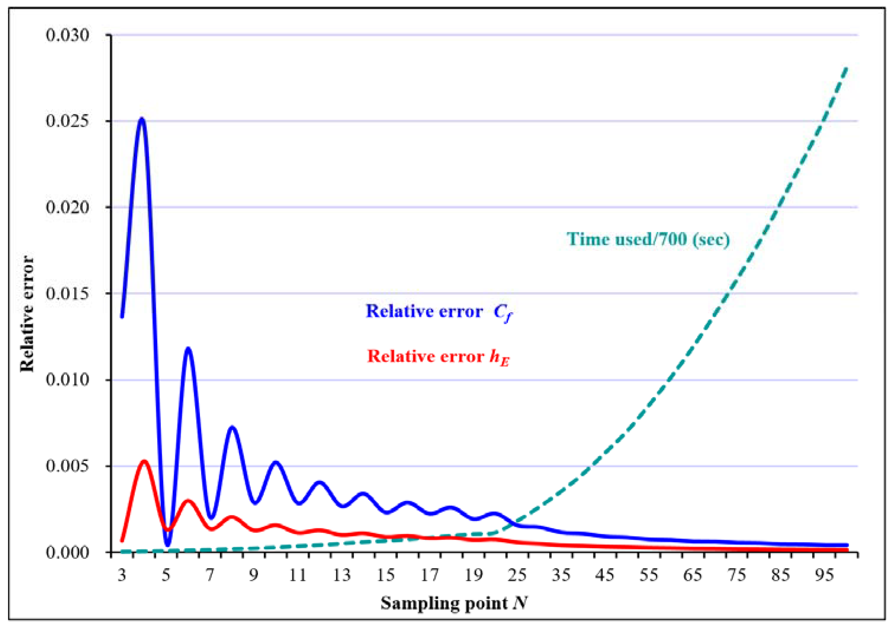
To observe the numerical calculation convergence law of the least squares curve-fitting method, the sampling time points are equally divided with a maximum time point of 1000 (h), and the relative error calculation results for C_f and h_E are given for an alternating distribution of positive and negative errors at the sampling points (see

Table 6. Calculation results for an alternating distribution of positive and negative errors at the sampling points.

Sampling Point N	Relative Error Cf	Relative Error hE	Time Used (s)
3	1.37 × 10−02	6.78 × 10−04	0.02
4	2.48 × 10−02	5.28 × 10−03	0.03
5	6.75 × 10−04	1.35 × 10−03	0.05
6	1.18 × 10−02	2.99 × 10−03	0.08
7	2.07 × 10−03	1.37 × 10−03	0.10
8	7.26 × 10−03	2.05 × 10−03	0.13
9	2.90 × 10−03	1.28 × 10−03	0.16
10	5.23 × 10−03	1.57 × 10−03	0.19
11	2.87 × 10−03	1.13 × 10−03	0.24
12	4.07 × 10−03	1.28 × 10−03	0.29
13	2.68 × 10−03	1.01 × 10−03	0.35
14	3.41 × 10−03	1.11 × 10−03	0.40
15	2.33 × 10−03	8.85 × 10−04	0.46
16	2.91 × 10−03	9.48 × 10−04	0.51
17	2.25 × 10−03	8.14 × 10−04	0.59
18	2.62 × 10−03	8.51 × 10−04	0.66
19	1.95 × 10−03	7.24 × 10−04	0.74
20	2.27 × 10−03	7.55 × 10−04	0.79
25	1.58 × 10−03	5.69 × 10−04	1.27
30	1.48 × 10−03	5.03 × 10−04	1.84
35	1.17 × 10−03	4.16 × 10−04	2.47
40	1.10 × 10−03	3.78 × 10−04	3.19
45	9.28 × 10−04	3.28 × 10−04	4.04
50	8.78 × 10−04	3.03 × 10−04	4.92
55	7.63 × 10−04	2.70 × 10−04	5.98
60	7.31 × 10−04	2.53 × 10−04	7.11
65	6.41 × 10−04	2.28 × 10−04	8.33
70	6.28 × 10−04	2.17 × 10−04	9.67
75	5.64 × 10−04	1.99 × 10−04	11.07
80	5.47 × 10−04	1.90 × 10−04	12.56
85	4.94 × 10−04	1.75 × 10−04	14.20
90	4.84 × 10−04	1.69 × 10−04	15.90
95	4.44 × 10−04	1.57 × 10−04	17.65
100	4.37 × 10−04	1.52 × 10−04	19.69

and Figure 6). When solving the equation corresponding to the least squares curve-fitting characteristic function (Formula (26)), the relative errors of C_f and h_E tend to decrease as the number of sampling points increases, and the time taken increases exponentially. For the convenience of observation, the “time used (s)” item in Figure 6 is reduced by a factor of 700.

It can be seen in Table 6 and Figure 6 that:

(1) The “relative error C_f” and “relative error h_E” decrease as the number of sampling points increases;

(2) For odd numbers of sampling points, the result is better than that for the adjacent even numbers; whether the number of nodes is odd or even, the more nodes that participate in the operation, the smaller the error;

(3) If one of the sampling points is used as the boundary to divide the positive and negative errors of the sampling points, the operation result is relatively poor. However, the more sampling points there are, the lower the probability of positive and negative error segmentation of such sampling points.

In summary, it can be seen from the derivation and testing of the numerical methods:

(1) When the measurement errors of all sampling points are the same or close, it can be seen in the characteristic function (Formula (16) or (26)) that the error of solution x and the comprehensive seepage parameter C_f is also smaller. However, it affects the value of h_E, and the error is determined by the measurement error;

(2) The more uniform the positive and negative error distributions are, the better the results of the least squares curve-fitting method are compared with those of the nonlinear-interpolation method;

(3) When the number of nodes involved in the calculation is three, the nonlinear-interpolation method is a special case of the least squares curve-fitting method. Therefore, the least squares curve-fitting method has wider adaptability.

4. Conclusions

(1) In accordance with the fluid-balance equation, a full-pumping state model and a nonfull-pumping state model are constructed. The dimensionality of the parameters other than time and the oil well submergence depth is reduced using the correlation characteristics of the seepage parameters, which effectively reduces the number of parameters in the models of submergence depth for oil wells during pumping and enhances the availability of this model.

(2) The relationship between the three types of oil wells and the two states are combed, the trends of the changes in the submergence depth in three phases (rising phase, holding phase, and falling phase) for the models of an oil well in the full and nonfull-pumping states are analyzed, and the judgment criteria for the corresponding submergence depth and the law governing the change in the pumping speed are given. On this basis, the criteria for transitioning an oil well from the full-pumping state to the nonfull-pumping state and from the nonfull-pumping state to the full-pumping state are given, which provides a basis for practical applications.

(3) For the nonlinear-interpolation method and the least squares curve-fitting method, the corresponding univariate characteristic equations are derived, and the unique existence of the solution of the characteristic equations in the (0, 1) interval is proven. The errors of the two numerical solution methods are estimated, the iteration times of the dichotomy are given, the relevant numerical solution tests and result analysis are carried out, and the possible adverse conditions of the sampling data are evaluated to provide a reference for avoiding such conditions.

(4) For the numerical-solution method of least squares curve-fitting, the computing environment was an Intel^® Core^TM i7-3770 CPU @ 3.40 GHz. When the number of sampling points was 10, 50, 100, 200, and 500, the time consumption was no more than 0.02, 0.6, 2, 7, and 45 s, respectively.

References

- Han, Y.; Song, X.; Li, K.; Yan, X. Hybrid modeling for submergence depth of the pumping well using stochastic configuration networks with random sampling. J. Pet. Sci. Eng. 2021, 208, 109423. [Google Scholar] [CrossRef]
- Xin, L.; Zhu-hong, Z. Research on Depth of Oil Well Moving Liquid Surface Based on Short-term Energy and LSTM. Comput. Mod. 2021, 04, 15–19. [Google Scholar] [CrossRef]
- Zhang, Y.; Wang, B. Determination of rational submergence depth of oil well pump. Oil Drill. Prod. Technol. 1999, 21, 62–65. [Google Scholar] [CrossRef]
- Qu, B.; Xu, H.; Ma, W.; Xu, Y. Impacts of submergence depth on overall performance of sucker rod pumping system. China Pet. Mach. 2015, 43, 89–93. [Google Scholar] [CrossRef]
- Dong, H.; Wu, T.; Liao, Q.; Chang, Z. Relationship between suitable submergence depth with pump efficiency. Inn. Mong. Petrochem. Ind. 2010, 36, 36–39. [Google Scholar] [CrossRef]
- Lin, X. Analysis of relation between sucker-rod working condition and submergence depth. Petrochem. Ind. Technol. 2016, 23, 99. [Google Scholar] [CrossRef]
- Wu, Q.; Han, L.; Wang, Y.; Fu, S. Influence factors of pump efficiency and determination of pump depth in deep well. Spec. Oil Gas Reserv. 2005, 12, 82–84. [Google Scholar] [CrossRef]
- He, L.; Jiashan, G.; Xueyan, W. Research on Reasonable Intermittent pumping System of oil Pumping Well. Oil Drill. Prod. Technol. 1900, 22, 69–72. [Google Scholar] [CrossRef]
- Fuchao, S.; Xiaohan, P.; Longda, L.; Fanfu, L.; Weina, J. Correction model research on oil well downhole flowrate test based on venturi. In Proceedings of the 33rd Chinese Control Conference, Nanjing, China, 28–30 July 2014; pp. 6664–6667. [Google Scholar] [CrossRef]
- Wang, H.B.; Dong, S.M.; Gan, Q.M.; Xin, H.; Zhu, G. Dynamic parameter simulation model of low-production pumping well and the ways to improve system efficiency. J. Acta Pet. Sin. 2018, 39, 1299–1307. [Google Scholar] [CrossRef]
- Zhang, Q.; Yan, X.; Shao, J. Fluid flow through anisotropic and deformable double porosity media with ultra-low matrix permeability: A continuum framework. J. Pet. Sci. Eng. 2021, 200, 108349. [Google Scholar] [CrossRef]
- Liu, T.; Zheng, M.; Song, X.; Wu, Y.; Zhang, R. Submergence depth modeling of oil well reservoirs and applications. J. Pet. Sci. Eng. 2021, 208, 109234. [Google Scholar] [CrossRef]
- Liu, T.; Lou, H.; Gao, X. Research on construction and application method of oil pumping speed control model. J. Xi’an Shiyou Univ. Nat. Sci. Ed. 2022, 37, 125–130. [Google Scholar] [CrossRef]
- Yu, D.; Qi, W.; Deng, S.; Zhang, Y.; Zhang, F.; Wang, X. Submergence forecasting of a submersible plunger pump based on the support vector machine. Acta Pet. Sin. 2011, 32, 53–538. [Google Scholar] [CrossRef] [Green Version]
- Li, X.; Tan, C.D.; Tan, P.F.; Zhang, S.L. Application of ARIMA Model in Time Series Analysisto Predict the Efficiency of Pumping Well Production System. Peak Data Sci. 2017, 6, 41–44. [Google Scholar] [CrossRef]
- Liu, T.; Zhao, Y.; Huang, Y. Research on the Submergence Depth Model of Oil Well Pumping. In Proceedings of the 2021 6th International Conference on Intelligent Computing and Signal Processing (ICSP), Xian, China, 9–11 April 2021; pp. 213–216. [Google Scholar]
- Liu, T.; Dong, Y. Research on numerical solution of one-sided monotonic function dichotomy. J. Phys. Conf. Ser. 2021, 2012. [Google Scholar] [CrossRef]
Figure 1.
Relationship between oil well types and pumping states.
Figure 2.
Schematic diagram of three-phase trends of the submergence depth in the full-pumping model.
Figure 3.
Schematic diagram of three-phase trends of the submergence depth in the nonfull-pumping model.
Figure 4.
Schematic diagram of transition from the full-pumping state to the nonfull-pumping state.
Figure 5.
Schematic diagram of transition from the nonfull-pumping state to the full-pumping state.
Figure 6.
Error trends of the least squares curve-fitting method with the number of sampling points.