A Semi-Analytical Model for Separating Diffuse and Direct Solar Radiation Components

Abstract

The knowledge of the solar irradiation components is required by most solar applications. When only the global horizontal irradiance is measured, this one is typically broken down into its fundamental components, beam and diffuse, by applying an empirical separation model. This study proposes a semi-analytical model for diffuse fraction, defined as the ratio of diffuse to global solar irradiance. Starting from basic knowledge, a general equation for diffuse fraction is derived. Clearness index, relative sunshine, and the clear-sky atmospheric transmittance are highlighted as robust predictors. Thus, the model equation implicitly provides hints for developing accurate empirical separation models. The proposed equation is quasi-universal, allowing for temporal (from 1-min to 1-day) and spatial (site specificity) customization. As a proof of theory, the separation quality is discussed in detail on the basis of radiometric data retrieved from Baseline Surface Radiation Network (BSRN), station Magurele, Romania. For temperate continental climate, overall results show for the diffuse fraction estimation a maximum possible accuracy around 7%, measured in terms of normalized root mean square error. One of the many options of implementing the semi-analytical model is illustrated in a case study.

1. Introduction

Energy generation from renewable sources has become a significant issue for the social and economic development of any community that aims to be sustainable. Many hopes are linked to the photovoltaic (PV) conversion of solar energy. Since solar energy is the cheapest fuel and a solar plant has a very low maintenance cost, PV plants have become widely spread across the globe as non-polluting power sources. This statement is argued by the weight of solar electricity in the energy mix, which, in the last years, experienced a sharp increase and this trend is expected to continue [1].

A PV plant project goes through two stages: development and exploitation. In the development stage, reliable solar resource statistics is required for the feasibility study and PV system design [2]. Solar energy collected on tilted surfaces is the physical quantity of main interest. Since only a very small number of radiometric stations record solar irradiance on tilted surfaces, numerical estimates are used in practice as substitute for measurements [3]. Generally, the solar irradiance components measured on a horizontal surface are transferred on the tilted surfaces by means of the so-called transposition models [4]. When only the global horizontal irradiance is measured, before applying a transposition model, it is broken down into its fundamental components: beam and diffuse. The operation is carried out by applying a separation model [5].

Following the pioneering work of the 1960s by Liu and Jordan [6], which reports an empirical equation that linearly connect daily diffuse and global solar irradiation, an abundance of separation models has been proposed. Almost all the separation models have an empirical basis of different deepness levels, going from purely empirical models [7] to the very rare models encapsulating features from the physics of the radiative transfer through the atmosphere [8]. Many empirical models are fitted on data collected from a limited geographical area (most of times a single location, e.g. [9]), which may dramatically limit their applicability only around the origin location. Other equations are fitted on data collected from a larger area, claiming a general applicability on a climate zone or even at a global level [10,11]. Aiming for increasing the separation accuracy, the very simple linear equation of Liu and Jordan [6], was replaced with more and more complicated equations: quadric [12], third order polynomial [13], exponential [14], separate equation per season [15], and so on. As far as the predictors are concerned, there is also a large diversity of separation models. Most of the empirical separation models express the diffuse fraction (see Section 2 for a definition) as a function of clearness index [16] and, sometimes, other atmospheric parameters (e.g. [17] considers 23 predictors, including some that account for the effect of clouds). From the timescale perspective, there are separation models that operate on data series of global solar irradiance ranging from 1-min sampling [7] to daily [18] or even monthly [19] sums. For more information about the separation models categories, we point the reader to Ref. [20] where a documented cross-classification is discussed.

The current state-of-the-art of the separation models is well captured by the recent work of Dazhi Yang [11]. The Yang’s paper evaluates the separation models developed after 2016, which claim a better performance than the Engerer2 model [21], which was found to be the best until 2016 [22]. The comprehensive review [22] compares the performance of 140 separation models using data from 54 locations from all climate zones. Whereas none of the models was found to be able to outperform the others in all locations, the Engerer2 model was found to be quasi-universal, based on statistical results averaged over different climate zones. Among the models developed after 2016, according to [11] the following four separating models (denoted as in [11]) demonstrated to be at least as efficient as the Engerer2 model: Yang4 [11], Starke1 [23], Starke3 [24], and Paulescu [7].

This study proposes a semi-analytical separation model. Starting from basic knowledge in modelling the atmospheric transmittance, a general equation for diffuse fraction is derived. Deeply different from previous models, the equation is derived without any empirical approach. The proposed model evaluates the diffuse fraction as a function of three parameters: the traditional clearness index, relative sunshine, and the mean atmospheric transmittance. The distinctive features of the proposed model are: (a) establishes a general analytical equation for a separation model. This is a formal equation which can be expanded and adapted for specific utilizations. (b) Based on physical criteria, the parameters that must be considered in the development of an accurate empirical separation model, are indicated, (c) the model is quasi-universal, allowing for temporal (from 1-min to 1-day) and spatial (location specificity) customization. Based on a numerical study, the quality of the separation process is discussed from different perspectives (timescale operation, state-of-the-sky, atmospheric transmittance) and its limits are evaluated.

The paper is organized as follows. Section 2 introduces the proposed semi-analytical model. A numerical proof of theory is discussed in detail in Section 3 at three sampling levels: 1-min, 1-h, and daylight. Section 4 is devoted to a case study focused on using as inputs mean atmospheric transmittances estimated with a clear-sky solar irradiance model. The main conclusions are gathered in Section 5.

2. Proposal for a Separation Model

The separation models typically estimate the diffuse fraction $k_d$, defined as the ratio of diffuse solar irradiation $H_d$ to global solar irradiation H:

$$k_d=\frac{H_d}{H}$$

(1)

As the introduction specifies, almost all empirical separation models express $k_d$ as a function of clearness index $k_t$ and other atmospheric parameters. Clearness index is defined as the ratio of global solar irradiation H measured at the ground to its counterpart at the top of the atmosphere $H_{ext}$:

$$k_t=\frac{H}{H_{ext}}$$

(2)

This section introduces a semi-analytical model derived from the basic theory of modeling solar radiation at the ground level.

The well-known closure relation between the solar irradiation components measured in a horizontal surface is:

$$H=H_b+H_d$$

(3)

On the basis of the results from [25], the beam solar irradiation $H_b$ can be approximated as:

$$H_b\cong \sigma H_{b0}$$

(4)

where $H_{b0}$ is the beam solar irradiation recorded in clear sky conditions. $\sigma =SD/\Delta t$ denotes the relative sunshine during a time interval $\Delta t$, i.e., the ratio between the sunshine duration SD and the greatest possible time of sunshine $\Delta t$. By way of consequence, if the Sun shines during $\Delta t$ then $\sigma =1$ and if the sky is overcast then $\sigma =0$. The consistency of the approximation was established on the basis of statistical theory [25]. Equation (4) is the sole approximation in this proof.

By using Equations (2)–(4) in the diffuse fraction definition (1), after elementary calculation it is obtained as:

$$k_d=1-\frac{\sigma }{k_t}\frac{H_{b0}}{H_{ext}}$$

(5)

At a generic level, the beam solar irradiation component under clear sky can be expressed as a function of the atmospheric transmittance ${\tau }_a$ (e.g. [26]):

$$H_{b0}=G_{SC}{\epsilon }_j{\displaystyle \underset{\Delta \omega }{\int }{\tau }_a\left(\omega \right)\sin hd\omega }$$

(6)

where $G_{SC}=1366.1\mathrm{W}/{\mathrm{m}}^2$ is the solar constant, ${\epsilon }_j$ denotes the correction of solar constant with respect to the Sun–Earth distance, h is the Sun elevation angle and ω represents the hour angle. During a given time interval $\Delta t$, $H_{ext}$ can be deterministically calculated:

$$H_{ext}=G_{SC}{\epsilon }_j{\displaystyle \underset{\Delta \omega }{\int }\sin hd\omega }$$

(7)

By summing up the results, it is obtained:

$$k_d=1-\frac{\sigma }{k_t}{\overline{\tau }}_a$$

(8)

where ${\overline{\tau }}_a=\frac{{\displaystyle \underset{\Delta \omega }{\int }{\tau }_a\left(\omega \right)\sin hd\omega }}{{\displaystyle \underset{\Delta \omega }{\int }\sin hd\omega }}$ represents the weighted average of the atmospheric transmittance with respect to the Sun’s elevation angle. Equation (8) is applicable for any time interval $\Delta t$ during a day.

Equation (8) represents a basic relationship between the diffuse fraction and three potential estimators: clearness index $k_t$, relative sunshine σ, and the mean value of the clear-sky atmospheric transmittance ${\overline{\tau }}_a$. The three estimators are not independent. $k_t$ and σ are strongly related (roughly linear) through the Ångström–Prescott equation [27,28] (see [29] for a recent review). Both $k_t$ and σ are not completely independent of ${\overline{\tau }}_a$, the relationships being weaker than the Ångström–Prescott equation but more complex. Even if Equation (8) is not directly useful in practice, it points out the parameters that should be considered in an empirical equation for diffuse fraction. Thus, along with the traditional predictors, clearness index and/or relative sunshine, the insertion into the diffuse fraction of some atmospheric parameters can contribute to improving the performance in the empirical estimation of diffuse fraction. These parameters are the same as those used in modeling the atmospheric transmittance in the clear-sky solar irradiance modeling, such as water vapor column content, Ångström parameters, etc. An analysis on this line is presented in Section 4, but before that the validation of the general equation, Equation (8), is compulsory.

3. Numerical Proof of the Theory

This proof intends to show that Equation (8) can be fitted with high accuracy on measured data, emphasizing its strengths and weaknesses. We chose to check it on a series of hourly data. On the one side, hourly sampling is usual in solar irradiation modeling, and, on the other side, $\Delta t=1\mathrm{h}$ can be regarded as an arbitrary chosen value of $\Delta t$ within a day. The boundary cases $\Delta t=0$ (instantaneous diffuse fraction) and $\Delta t=\mathrm{daylight}\_\mathrm{length}$ are discussed too. The models’ performance is evaluated using two statistical indicators, normalized root mean square error (nRMSE) and normalized mean bias error (nMBE). The two indicators are defined in Appendix A.

3.1. Data

The study was conducted with high-quality radiometric data retrieved from BSRN–- Baseline Surface Radiation Network, station Magurele, Romania [30].

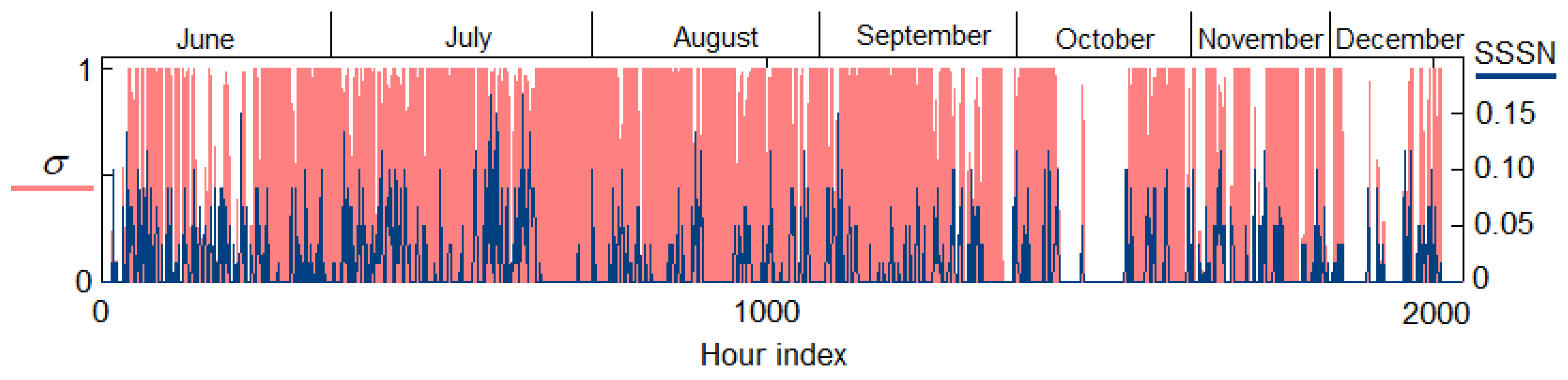
The town Magurele (44.3439 N; 26.0123 E, 110 m asl) is located in a rural area, close to the capital Bucharest. Magurele experiences a transitional climate, with both continental and subtropical influences (Koppen climate classification Cfa [31]). Global, diffuse, and direct-normal solar irradiances recorded at 1-min resolution during 1 June to 31 December 2021, were used to build the specific database. A carefully quality check was performed, at the first step the suspicious data being removed. At the second step, only data measured at the Sun elevation angle h > 5° were selected (the pyranometers accuracy is questionable close to sunrise and sunset). Finally, only those hours containing a complete dataset (60 measurements points) were retained. This dataset, further denoted hDATA, was completed with physical quantities resulted from post-processing of measurements, e.g., relative sunshine σ, clearness index, sunshine number SSN (as a proxy for relative sunshine), and sunshine stability number SSSN (as a quantifier for the variability in the state-of-the-sky). SSN and SSSN are defined in Appendix B. Figure 1 shows the variation of σ and SSSN for all 2044 valid hours comprised in hDATA. Visual inspection of Figure 1 highlights the complexity of the hDATA dataset. It contains both hours with stable clear or overcast skies, partly sunny hours with moderate variability in the-state-of-the-sky, but also hours with a high degree of variability in the-state-of-the-sky occurring either on a clear-sky or cloudy background. Similar databases were built for evaluating the boundary cases $\Delta t=0$ (iDATA) and $\Delta t=\mathrm{daylight}\_\mathrm{length}$ (dDATA).

3.2. Model Assessment at 1-Hour Sampling

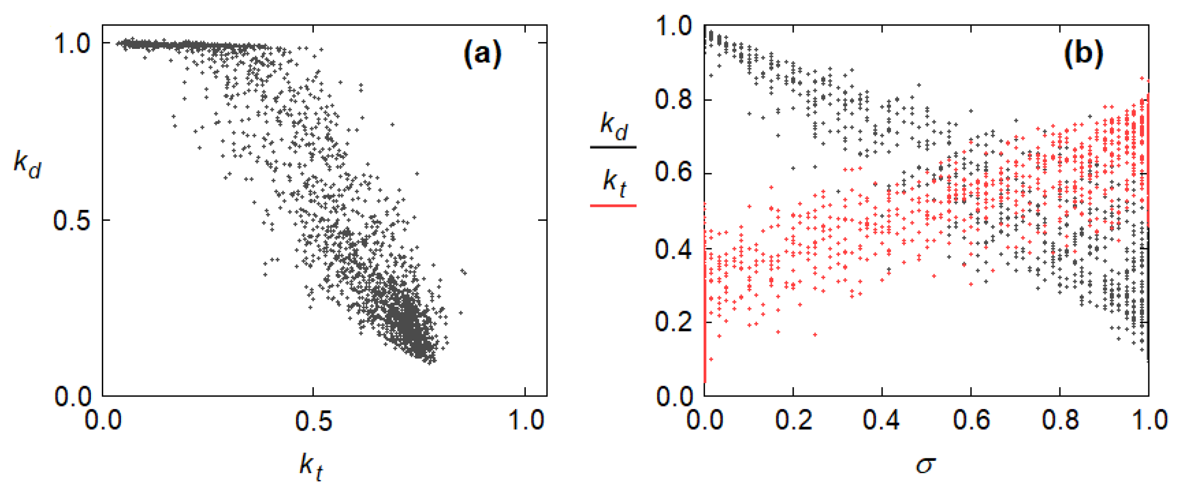
The results of applying Equation (8) to hDATA are assessed next. First, a brief analysis of the variables is presented. Figure 2a shows a typical picture of $k_d-k_t$ scattering. Clearness index varies from values lower than 0.1, recorded in hours with the Sun covered by opaque clouds, to values around 0.75, recorded in clear sky hours. The points are clustered in two regions: $k_d\simeq 1$, corresponding to the Sun covered by clouds and, roughly, $0.1<k_d<0.2$ corresponding to a bright Sun on the sky. The cloud transmittance has a lower influence on diffuse fraction ($k_d\simeq 1$ for most values of $k_t<0.4$). Differently, in sunny conditions (high values of $k_t$), $k_d$ experiences a large dispersion, indicated a strong influence of the clear-sky atmospheric transmittance on the diffuse fraction. These observations are substantiated in Figure 2b, where $k_d$ is plotted against relative sunshine σ. While, in the mostly cloudy sky hours, a low dispersion of $k_d$ is noted, in the mostly sunny hours, a large dispersion of $k_d$ is noted. The clear-sky atmospheric transmittance ${\overline{\tau }}_a$ in Equation (8) is expected just to cover the scattering on mostly clear sky hours.

There is a wide range of options for estimating ${\overline{\tau }}_a$. First, only those hours in which a variable sky $0<\sigma <1$ was recorded, are considered. The cases $\sigma =0$ and $\sigma =1$ are discussed separately. The two limits are neither trivial nor minimalist. The partition of hDATA looks like this: 470 data recorded in overcast conditions $\sigma =0$, 730 in variable sky $0<\sigma <1$ and 844 in sunny conditions $\sigma =1$. At least in temperate climate, approximately half of daylight hours are either sunny or overcast, emphasizing the substantial role of the two limits in the overall performance of a separation model. Most of the empirical separation equations cover the entire range of relative sunshine, even if at the limits $\sigma =0$ and $\sigma =1$, Equation (8) is reduced to very specific forms according to the physical phenomenology. For more inside this topic, we point the reader to [32] where the limits $\sigma =0$ and $\sigma =1$ are analyzed in the analogue context of the Ångström–Prescott equation.

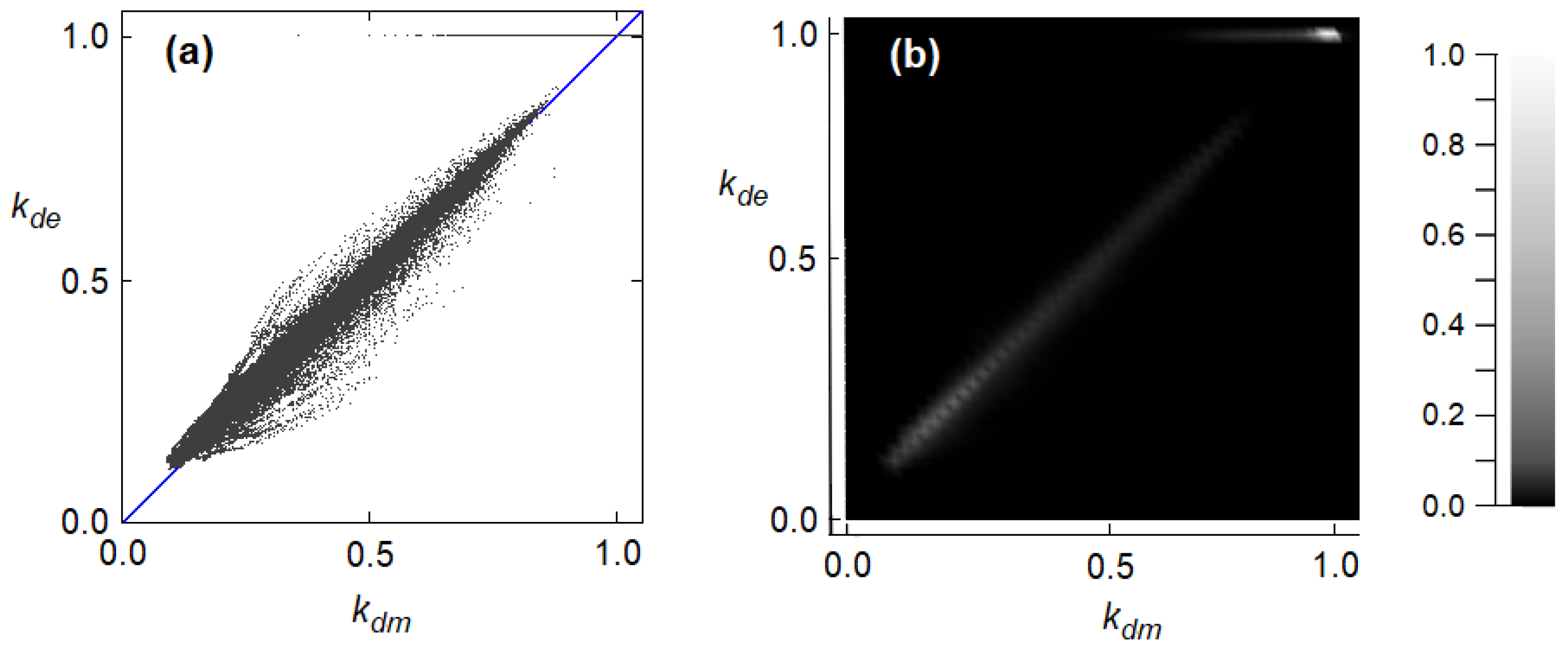
Under variable sky conditions $0<\sigma <1$, two approximations of ${\overline{\tau }}_a$ are discussed next. In the first case, ${\overline{\tau }}_a$ was evaluated as an average value over the entire period. For this, a linear Ångström–Prescott equation, $k_t=a+b\sigma$, was fitted on data (Figure 2b), then ${\overline{\tau }}_a$ being simply evaluated as ${\overline{\tau }}_a=a+b$, i.e., ${\overline{\tau }}_a=0.3038+0.3794=0.6833$ (see e.g. [29] for details). Figure 2b shows a typical picture of $k_t$ with respect to σ, emphasizing the linear nature of the Ångström–Prescott equation. In the second case, ${\overline{\tau }}_a$ was evaluated hour by hour on the basis of direct-normal solar irradiance measured data series. It is worth reminding that in this case only those hours in which $0<\sigma <1$ were considered, so that for at least one minute the Sun shined on the sky, allowing for direct-normal solar irradiance measurement. The results are gathered in Figure 3 in the form of scatter plots. Visual inspection of Figure 3 shows the high influence of the clear-sky atmospheric transmittance on the accuracy of diffuse fraction estimation. Thus, assuming a long-term average for ${\overline{\tau }}_a$ in Equation (8) leads to a severe underestimation of measured data (Figure 3a). If hourly averages of atmospheric transmittance are considered (Figure 3b), a high accuracy in diffuse fraction estimation is noted (nMBE= 0.053 and nRMSE = 0.067). The estimates accuracy can be further increased if ${\overline{\tau }}_a$ is calculated as the theory prescribes, i.e., as a weighted average with respect to the Sun elevation angle.

At the sunny-sky limit $\sigma =1$, Equation (8) reduces to $k_d=1-{\overline{\tau }}_a/k_t$. Figure 3b also displays estimated (assuming hourly mean for ${\overline{\tau }}_a$) vs. measured $k_d$ in this case. The model performance drops by half: nMBE = 0.099 and nRMSE = 0.125. A possible cause could be the presence of clouds close to the Sun or a thin layer of clouds covering the Sun generating the so-called cloud enhancement events [33].

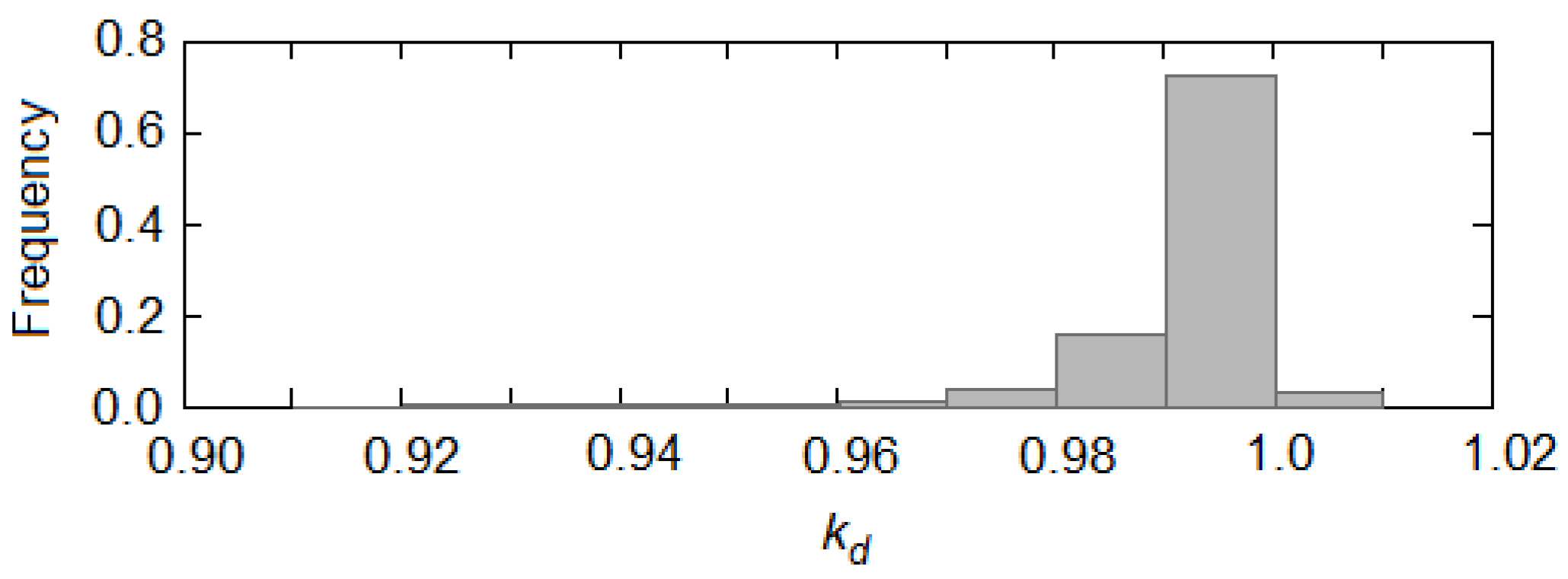
At the overcast limit $\sigma =0$, Equation (8) estimates always $k_d=1$, which is theoretically sound (when the Sun is covered by clouds the global solar irradiance equals diffuse solar irradiance). The measurements of $k_d$ experience values closer but different from one. Figure 4 shows a histogram of measured $k_d$ for $\sigma =0$. Majority of the values are clustered between 0.99 and 1.01, approx. 80%). The statistical indicators nMBE = 0.009 and nRMSE = 0.013 substantiate the model’s assumption $k_d=1$ for $\sigma =0$.

Summing up the results and computing the statistical indicators of accuracy over the entire database we obtained: nMBE = 0.043 and nRMSE = 0.058. This is a remarkable result, emphasizing the high-performance of Equation (8) in capturing the reality.

3.3. Extreme Cases

The study presented in Section 3.2 was performed assuming an hourly sampling,$\Delta t=1\mathrm{h}$. The following question remains: how do the results change when $\Delta t$ deviates considerably from one hour. The results presented next answer this question, the focus being on the extreme cases $\Delta t=0$ (instantaneous diffuse fraction) and $\Delta t=\mathrm{daylight}\_\mathrm{length}$.

Diffuse fraction of solar irradiance ($\Delta t=0$) is a very specific subject-matter, closely related to the clear-sky solar irradiance modeling. When $\Delta t\to 0$, the physical quantities in Equation (8) change to instantaneous quantities, i.e., $\sigma \to \mathrm{SSN}$(see Appendix B for SSN definition) and the mean atmospheric transmittance ${\overline{\tau }}_a$ tends to the instantaneous value ${\tau }_a$. Thus, Equation (8) becomes:

$$k_d=\{\begin{array}{ll}1-\frac{1}{k_t}{\tau }_a& \mathrm{IF}SSN=1\\ 1& \mathrm{IF}SSN=0\end{array}$$

(9)

Always when the Sun is covered by clouds (SSN = 0), Equation (9) estimates $k_d=1$, which is theoretically sound. When the Sun shines (SSN = 1), Equation (9) preserves the complex dependence on the atmospheric transmittance. It should be noted that the clearness index $k_t$ in Equation (9) is a measured quantity, being the common parameter of the empirical separation models. Thus, aiming to empirically develop a separation model, the atmospheric transmittance ${\tau }_a$ may be the subject of an empirical parameterization.

Figure 5 shows the instantaneous diffuse fraction evaluated based on the measurements comprised by iDATA dataset. iDATA contains 139,023 measurement points, recorded at 1-min sampling, the native resolution of BSRN. The points distribution on the $k_d-k_t$ plane (Figure 5a) is like that observed for hourly diffuse fraction (Figure 2a), but a much larger dispersion is observed. Without any averaging, the impact on the global solar irradiance of the atmospheric transmittance (measured on the Sun direction), cloud enhancement, pyranometers uncertainties is more prominent.

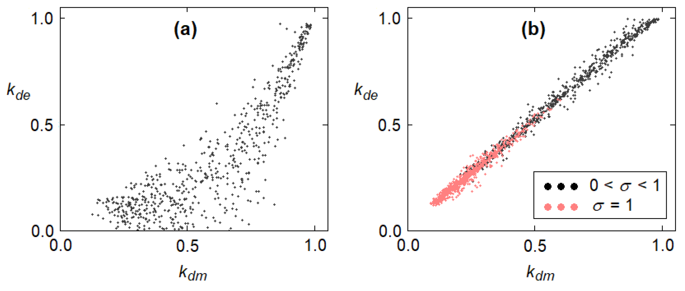
However, visual inspection of the density plot from Figure 5b, shows a clustering of the points in two regions: Sun covered by clouds (roughly 33% of iDATA for $k_d>0.95$) and almost clear sky (roughly 45% of iDATA for $k_d<0.25$ and $0.6<k_t<0.8$). Figure 5b is consistent to other studies (e.g., [24]) but combined with Equation (9) emphasize the weight of the two clusters for ${\tau }_a$ parameterization. The ability of Equation (9) in capturing the peculiarities of instantaneous diffuse fraction is illustrated in Figure 6a. The points corresponding to the SSN = 1 branch in Equation (9) (roughly 60%) are clustered around the first diagonal while the points corresponding to the SSN = 0 branch (roughly 40%) are distributed on a horizontal line segment, the estimated $k_d=1$. The density plot from Figure 6b shows that most of the points are clustered very close to the first diagonal and the measured value $k_d=1$. In terms of statistical indicators, Equation (9) applied to iDATA achieves: nRMSE = 0.074 and nMBE = 0.035. As it was developed, the inherent measurement errors, the cloud enhancement phenomena are not considered by Equation (9). An empirical parameterization of ${\tau }_a$ could capture features from the cloud enhancement.

If we compare this result with the ones from [11], we even find a very good performance of the model defined by Equation (8). According to [11], the current best model reaches temperate climate performances ranging between nRMSE = 0.247 and nRMSE = 0.649. In other words, by using Equation (8) nRMSE can drop three times compared to the most performing current models.

At the other frontier, $\Delta t$ equals to the daylength, the diffuse fraction is estimated by Equation (8). The test performed on dDATA dataset (with ${\overline{\tau }}_a$ calculated as a weighted average over the entire day) led to nRMSE = 0.078 and nMBE = 0.003. Comparing to the case of hourly sampling, a larger scattering in noted but the bias is removed.

To this end, it is worth to note that the proof presented above considers a knowledge of the average atmospheric transmittance with the highest accuracy, ${\overline{\tau }}_a$ being the result of direct measurement. As a consequence, the calculated values of nRMSE and nMBE can be considered as reliable indicators for the accuracy limit of the proposed semi-analytical model.

4. Practical Implementation: Case Study

Equation (8) is general, there being almost unlimited ways to customize it. The general equation can be substituted purely with empirical models based on the predictors formalized in the Equation (8) inference. Another option could be keeping the form of Equation (8) and expressing ${\overline{\tau }}_a$ as a function of the available atmospheric parameters. There are a large variety of clear-sky solar irradiance models that can be integrated for ${\overline{\tau }}_a$ [34]. The accuracy of ${\overline{\tau }}_a$ estimation depends on the clear-sky solar irradiance model and it can be conditioned by several factors, such as the atmospheric parameters availability, the measurements quality, and so on.

This section presents a case study focused on the latter version. The assumptions underlying the study are the following:

(1)

The aim is to estimate the hourly mean diffuse solar irradiance at the station Magurele, Romania, briefly described in Section 3.1;

(2)

The estimation of diffuse fraction is made based on Equation (8), using the PSα clear-sky solar irradiance model [35] for evaluating ${\overline{\tau }}_a$.

(3)

Global solar irradiance and sunshine duration are measured in situ, enabling the calculation of the clearness index and relative sunshine, respectively. In particular, records from hDATA dataset are used;

(4)

For running PSα, the aerosol optical depth (AOD), the Ångström exponent α and the water vapor column content w are retrieved from the Aerosol Robotic Network (AERONET) [36] at daily resolution. The Ångström turbidity factor β is evaluated based on AOD and α (see e.g., [35] and the references therein for details).

(5)

For the ozone column content, a mean value of 0.35 cm⋅atm was assumed.

The results of testing this specific implementation of Equation (8) are collected in Figure 7. Visual inspection of Figure 7a shows a relatively large scatter of estimated vs. measured diffuse fraction (nRMSE = 0.245). No bias is observed (nMBE = −0.015). However, such a large scattering of data is characteristic of the separation models.

Table 1. Performance of different hourly diffuse fraction models applied to hDATA dataset.

Model Reference	[37]	[38]	[39]	[40]	[41]	[42]	[43]	[16]	[17]
nRMSE	0.281	0.281	0.263	0.260	0.270	0.254	0.266	0.280	0.302
nMBE	0.102	0.051	0.066	0.031	0.062	−0.013	−0.074	0.102	−0.153

shows the results of running different models for the diffuse fraction reported over time. The equations are various: triple segmented linear [37,38,39], triple segmented polynomials of order three [40] and four [41,42,43], exponential [16] and double segmented [17]. There is also a variety of places of origin: North America, South America, Australia, Europe, and Asia. The models performance ranges between nRMSE = 0.254 for a polynomial model of order 4 and nRMSE = 0.302 for the double segmented model. The specific implementation of Equation (8) combined with PSα keeps a small advance in front of these models. While all the models considered in this comparison hold frozen numerical coefficients, Equation (8) exhibit a large flexibility in implementation. There are many other possibilities of computing ${\overline{\tau }}_a$ that can lead more or less to better results.

The final outcome of the separation process is the hourly diffuse solar irradiance. This is evaluated in Figure 7b, also as a scatter plot. Comparing with the diffuse fraction, a slight decreasing in the estimation accuracy can be observed (nRMSE = 0.313 and nMBE = −0.046). It is worth emphasizing that the majority of points are clustered in a lenticular domain around the first diagonal. There is a very small number of points where the diffuse irradiance is estimated with large errors. Since nRMSE is a statistical indicator that penalizes errors more drastically as they increase, the weight of this small number of errors has a major contribution in establishing the nRMSE value. Looking at the proposed model precision, measured by the percentage p [%] of estimates accurate to within a given tolerance interval TOL [%], it appears very good: p [TOL = 10%] = 36.7% while p [TOL = 20%] = 59.6%.

5. Conclusions

The relevance of the models for separating the global irradiance into its direct and diffuse components is highlighted by the large number of scientific reports on this topic. The majority of the reported separation models are built empirically, paying tribute to the location of origin. Starting from basic knowledge in modelling the atmospheric transmittance, a general equation for diffuse fraction is derived, namely Equation (8). Deeply different from previous models, the equation is derived without any empirical approach. Clearness index, relative sunshine, and the mean clear-sky atmospheric transmittance are identified as primary predictors for a separation model. A numerical proof of theory is presented in detail in Section 3. This proof assumes the knowledge of the mean atmospheric transmittance with the highest possible accuracy, being the result of direct measurement. Therefore, the calculated value of normalized root mean square error can be considered as a reliable indicator of the maximum accuracy that can be achieved by the proposed semi-analytical model. For temperate continental climate, overall results show a limit of accuracy for the estimation of diffuse fraction around 7%, measured in terms of normalized root mean square error.

Equation (8) can be applied directly in practice as it is. But Equation (8) have a great merit in the development of an empirical separation model. It formally indicates the optimal equation and the optimal predictors necessary to explain the high variability commonly experienced by the measured diffuse fraction. While the clearness index is a mandatory predictor (global solar irradiance is always supposed to be known), there is plenty of room for adapting the model according to the atmospheric data availability aiming to an accurate calculation of the mean atmospheric transmittance.

The proposed separation model can be regarded as general, allowing for temporal (from 1-min to 1-day) and spatial (site specificity) customization. This study was focused on its development, proof of the theory, and an estimation of the theoretical limit of accuracy. Many facets of research are still open. A verification at the global scale of the semi-analytical separation model (assuming different implementations of different complexities) is planned in the immediate future.

References

- Solar Power Europe. EU Market Outlook for Solar Power 2021–2025. 2021. Available online: https://www.solarpowereurope.org/insights/market-outlooks (accessed on 1 September 2022).
- Rehman, S.; Ahmed, M.A.; Mohamed, M.H.; Al-Sulaiman, F.A. Feasibility study of the grid connected 10MW installed capacity PV power plants in Saudi Arabia. Renew. Sustain. Energy Rev. 2017, 80, 319–329. [Google Scholar] [CrossRef]
- Kambezidis, H.D.; Psiloglou, B.E. Estimation of the Optimum Energy Received by Solar Energy Flat-Plate Convertors in Greece Using Typical Meteorological Years. Part I: South-Oriented Tilt Angles. Appl. Sci. 2021, 11, 1547. [Google Scholar] [CrossRef]
- Yang, D. Solar radiation on inclined surfaces: Corrections and benchmarks. Sol. Energy 2016, 136, 288–302. [Google Scholar] [CrossRef]
- Paulescu, E.; Blaga, R. Regression models for hourly diffuse solar radiation. Sol. Energy 2016, 125, 111–124. [Google Scholar] [CrossRef]
- Liu, B.; Jordan, R. The interrelationship and characteristic distribution of direct, diffuse and total solar radiation. Sol. Energy 1960, 4, 1–19. [Google Scholar] [CrossRef]
- Paulescu, E.; Blaga, R. A simple and reliable empirical model with two predictors for estimating 1-minute diffuse fraction. Sol. Energy 2019, 180, 75–84. [Google Scholar] [CrossRef]
- Hollands, K.G.T.; Crha, S.J. An improved model for diffuse radiation: Correction for atmospheric back-scattering. Sol Energy 1987, 38, 233–236. [Google Scholar] [CrossRef]
- Lewis, G. Estimates of monthly mean daily diffuse irradiation in the Southeastern United States. Renew. Energy 1995, 6, 983–988. [Google Scholar] [CrossRef]
- Yang, D. Temporal-resolution cascade model for separation of 1-min beam and diffuse irradiance. J. Renew. Sustain. Energy 2021, 13, 056101. [Google Scholar] [CrossRef]
- Yang, D. Estimating 1-min beam and diffuse irradiance from the global irradiance: A review and an extensive worldwide comparison of latest separation models at 126 stations. Renew. Sustain. Energy Rev. 2022, 159, 112195. [Google Scholar] [CrossRef]
- Haydar, A.; Balli, O.; Hepbasli, A. Estimating the horizontal diffuse solar radiation over the Central Anatolia region of Turkey. Energy Convers. Manag. 2006, 47, 2240–2249. [Google Scholar]
- Tarhan, S.; Sari, A. Model selection for global and diffuse radiation over the Central Black Sea (CBS) region of Turkey. Energy Convers. Manag. 2005, 46, 605–613. [Google Scholar] [CrossRef]
- Boukelia, T.E.; Mecibah, M.-S.; Meriche, I.E. General models for estimation of the monthly mean daily diffuse solar radiation (Case study: Algeria). Energy Convers. Manag. 2014, 81, 211–219. [Google Scholar] [CrossRef]
- Paliatsos, A.G.; Kambezidis, H.D.; Antoniou, A. Diffuse solar irradiation at a location in the Balkan Peninsula. Renew. Energy 2003, 28, 2147–2156. [Google Scholar] [CrossRef]
- Boland, J.; Scott, L.; Luther, M. Modelling the diffuse fraction of global solar radiation on a horizontal surface. Environmetrics 2001, 12, 103–116. [Google Scholar] [CrossRef]
- Furlan, C.; Pereira de Oliveira, A.; Soares, J.; Codato, G.; Escobedo, J.F. The role of clouds in improving the regression model for hourly values of diffuse solar radiation. Appl. Energy 2012, 92, 240–254. [Google Scholar] [CrossRef]
- Bortolini, M.; Gamberi, M.; Graziani, A.; Manzini, R.; Mora, C. Multi-location model for the estimation of the horizontal daily diffuse fraction of solar radiation in Europe. Energy Convers. Manag. 2013, 67, 208–216. [Google Scholar] [CrossRef]
- Karakoti, I.; Das, P.K.; Singh, S.K. Predicting monthly mean daily diffuse radiation for India. Appl. Energy 2012, 91, 412–425. [Google Scholar] [CrossRef]
- Khorasanizadeh, H.; Mohammadi, K. Diffuse solar radiation on a horizontal surface: Reviewing and categorizing the empirical models. Renew. Sust. Energy Rev. 2016, 53, 338–362. [Google Scholar] [CrossRef]
- Engerer, N.A. Minute resolution estimates of the diffuse fraction of global irradiance for southeastern Australia. Sol. Energy 2015, 116, 215–237. [Google Scholar] [CrossRef]
- Gueymard, C.A.; Ruiz-Arias, J.A. Extensive worldwide validation and climate sensitivity analysis of direct irradiance predictions from 1-min global irradiance. Sol. Energy 2016, 128, 1–30. [Google Scholar] [CrossRef]
- Starke, A.R.; Lemos, L.F.L.; Boland, J.; Cardemil, J.M.; Colle, S. Resolution of the cloud enhancement problem for one-minute diffuse radiation prediction. Renew. Energy 2018, 125, 472–484. [Google Scholar] [CrossRef]
- Starke, A.R.; Lemos, L.F.L.; Barni, C.M.; Machado, R.D.; Cardemil, J.M.; Boland, J.; Colle, S. Assessing one-minute diffuse fraction models based on worldwide climate features. Renew. Energy 2021, 177, 700–714. [Google Scholar] [CrossRef]
- Stefu, N.; Paulescu, M.; Blaga, R.; Calinoiu, D.; Pop, N.; Boata, R.; Paulescu, E. A theoretical framework for Ångström equation. Its virtues and liabilities in solar energy estimation. Energy Convers. Manag. 2016, 112, 236–245. [Google Scholar] [CrossRef]
- Paulescu, E.; Paulescu, M. A new clear sky solar irradiance model. Renew. Energy 2021, 179, 2094–2103. [Google Scholar] [CrossRef]
- Ångström, A. Solar and ter restrial radiation. Report to the international commission for solar research on actinometric investigations of sola and atmospheric radiation. Q. J. R. Meteor. Soc. 1924, 50, 121–126. [Google Scholar] [CrossRef]
- Prescott, J.A. Evaporation from a water surface in relation to solar radiation. Trans. R. Soc. S. Aust. 1940, 64, 114–118. [Google Scholar]
- Paulescu, M.; Stefu, N.; Calinoiu, D.; Paulescu, E.; Pop, N.; Boata, R.; Mares, O. Ångström–Prescott equation: Physical basis, empirical models and sensitivity analysis. Renew. Sustain. Energy Rev. 2016, 62, 495–506. [Google Scholar] [CrossRef]
- Baseline Surface Radiation Network (BSRN). Available online: https://bsrn.awi.de/ (accessed on 1 September 2022).
- Kottek, M.; Grieser, J.; Beck, C.; Rudolf, B.; Rubel, F. World Map of the Köppen-Geiger climate classification updated. Meteorol. Z. 2006, 15, 259–263. [Google Scholar] [CrossRef]
- Brabec, M.; Badescu, V.; Dumitrescu, A.; Paulescu, M. A new point of view on the relationship between global solar irradiation and sunshine quantifiers. Sol. Energy 2016, 126, 252–263. [Google Scholar] [CrossRef]
- Järvelä, M.; Lappalainen, K.; Valkealahti, S. Characteristics of the cloud enhancement phenomenon and PV power plants. Sol. Energy 2020, 196, 137–145. [Google Scholar] [CrossRef]
- Sun, X.; Bright, J.M.; Gueymard, C.A.; Bai, X.; Acord, B.; Wang, P. Worldwide performance assessment of 95 direct and diffuse clear-sky irradiance models using principal component analysis. Renew. Sustain. Energy Rev. 2021, 135, 110087. [Google Scholar] [CrossRef]
- Blaga, R.; Calinoiu, D.; Paulescu, M. A one-parameter family of clear-sky solar irradiance models adapted for different aerosol types. J. Renew. Sustain. Energy 2021, 13, 023701. [Google Scholar] [CrossRef]
- Aerosol Robotic Network. AERONET. 2022. Available online: https://aeronet.gsfc.nasa.gov/ (accessed on 1 September 2022).
- Orgill, J.F.; Hollands, K.G.T. Correlation equation for hourly diffuse radiation on a horizontal surface. Sol. Energy 1977, 19, 357–359. [Google Scholar] [CrossRef]
- Lam, J.C.; Li, D.H.W. Regression Analysis of Solar Radiation and Sunshine Duration. Archit. Sci. Rev. 1996, 39, 15–23. [Google Scholar] [CrossRef]
- Reindl, D.T.; Beckman, W.A.; Duffe, J.A. Diffuse fraction correlations. Sol. Energy. 1990, 45, 1–7. [Google Scholar] [CrossRef]
- Jacovides, C.P.; Tymvios, F.S.; Assimakopoulos, V.D.; Kaltsounides, N.A. Comparative study of various correlations in estimating hourly diffuse fraction of global solar radiation. Renew. Energy 2006, 31, 2492–2504. [Google Scholar] [CrossRef]
- Erbs, D.G.; Klein, S.A.; Duffie, J.A. Estimation of the diffuse radiation fraction for hourly, daily and monthly-average global radiation. Sol. Energy 1982, 28, 293–302. [Google Scholar] [CrossRef]
- Oliveira, A.P.; Escobedo, J.F.; Machado, A.J.; Soares, J. Correlation models of diffuse solar-radiation applied to the city of Sao Paulo, Brazil. Appl. Energy 2002, 71, 59–73. [Google Scholar] [CrossRef]
- Soares, J.; Oliveira, A.P.; Boznar, M.Z.; Mlakar, P.; Escobedo, J.F.; Machado, A.J. Modeling hourly diffuse solar-radiation in the city of Sao Paulo using a neural-network technique. Appl. Energy 2004, 79, 201–214. [Google Scholar] [CrossRef]
- Badescu, V.; Paulescu, M. Statistical properties of the sunshine number illustrated with measurements from Timisoara (Romania). Atmos. Res. 2011, 101, 194–204. [Google Scholar] [CrossRef]
- World Meteorological Organization. Guide to Meteorological Instruments and Methods of Observation. WMO-No.8/2008. 2022. Available online: https://community.wmo.int/activity-areas/imop/wmo-no_8 (accessed on 1 September 2022).
- Paulescu, M.; Badescu, V. New approach to measure the stability of the solar radiative regime. Theor. Appl. Climatol. 2011, 103, 459–470. [Google Scholar] [CrossRef]
- Blaga, R.; Paulescu, M. Quantifiers for the solar irradiance variability: A new perspective. Sol. Energy 2018, 174, 606–616. [Google Scholar] [CrossRef]
Figure 1.
Relative sunshine σ (red) and sunshine stability number SSSN (blue) recorded in each hour from the hDATA database.
Figure 2.
Graphical presentation of the relationships between the physical quantities involved in Equation (8): (a) Diffuse fraction with respect to clearness index ; (b) diffuse fraction and clearness index with respect to the relative sunshine σ. Post-processed data from hDATA are used.
Figure 3.
Estimated with Equation (8) vs. measured diffuse. The values of clear-sky atmospheric transmittance in Equation (8) are: (a) a long-term average and (b), hourly average.
Figure 4.
Distribution of measured in the hours from hDATA with the Sun covered by clouds, .
Figure 5.
(a) Instantaneous measured diffuse fraction with respect to measured clearness index . The entire iDADA dataset was used; (b) density plot of data from the frame (a).
Figure 6.
(a) Estimated with Equation (9) vs. measured diffuse fraction. (b) Density plot of data from the frame (a).
Figure 7.
(a) Estimated with Equation (8) vs. measured hourly diffuse fraction. (b) Estimated hourly averaged diffuse solar irradiance DHIe vs. measured hourly averaged diffuse solar irradiance DHIm.
Publisher’s Note: MDPI stays neutral with regard to jurisdictional claims in published maps and institutional affiliations. |
© 2022 by the authors. Licensee MDPI, Basel, Switzerland. This article is an open access article distributed under the terms and conditions of the Creative Commons Attribution (CC BY) license (https://creativecommons.org/licenses/by/4.0/).
Share and Cite
MDPI and ACS Style
Paulescu, E.; Paulescu, M. A Semi-Analytical Model for Separating Diffuse and Direct Solar Radiation Components. Appl. Sci. 2022, 12, 12759. https://0-doi-org.brum.beds.ac.uk/10.3390/app122412759
AMA Style
Paulescu E, Paulescu M. A Semi-Analytical Model for Separating Diffuse and Direct Solar Radiation Components. Applied Sciences. 2022; 12(24):12759. https://0-doi-org.brum.beds.ac.uk/10.3390/app122412759
Chicago/Turabian StylePaulescu, Eugenia, and Marius Paulescu. 2022. "A Semi-Analytical Model for Separating Diffuse and Direct Solar Radiation Components" Applied Sciences 12, no. 24: 12759. https://0-doi-org.brum.beds.ac.uk/10.3390/app122412759
Note that from the first issue of 2016, this journal uses article numbers instead of page numbers. See further details here.