
GeoBERT: Pre-Training Geospatial Representation Learning on Point-of-Interest

1
Shanghai Key Laboratory of Data Science, School of Computer Science, Fudan University, Shanghai 200433, China
2
College of Design and Innovation, Tongji University, Shanghai 200092, China
*
Author to whom correspondence should be addressed.
Appl. Sci. 2022, 12(24), 12942; https://0-doi-org.brum.beds.ac.uk/10.3390/app122412942
Submission received: 24 November 2022
/
Revised: 12 December 2022
/
Accepted: 12 December 2022
/
Published: 16 December 2022
(This article belongs to the Special Issue Natural Language Processing (NLP) and Applications)
Abstract
:Thanks to the development of geographic information technology, geospatial representation learning based on POIs (Point-of-Interest) has gained widespread attention in the past few years. POI is an important indicator to reflect urban socioeconomic activities, widely used to extract geospatial information. However, previous studies often focus on a specific area, such as a city or a district, and are designed only for particular tasks, such as land-use classification. On the other hand, large-scale pre-trained models (PTMs) have recently achieved impressive success and become a milestone in artificial intelligence (AI). Against this background, this study proposes the first large-scale pre-training geospatial representation learning model called GeoBERT. First, we collect about 17 million POIs in 30 cities across China to construct pre-training corpora, with 313 POI types as the tokens and the level-7 Geohash grids as the basic units. Second, we pre-train GeoEBRT to learn grid embedding in self-supervised learning by masking the POI type and then predicting. Third, under the paradigm of “pre-training + fine-tuning”, we design five practical downstream tasks. Experiments show that, with just one additional output layer fine-tuning, GeoBERT outperforms previous NLP methods (Word2vec, GloVe) used in geospatial representation learning by 9.21% on average in F1-score for classification tasks, such as store site recommendation and working/living area prediction. For regression tasks, such as POI number prediction, house price prediction, and passenger flow prediction, GeoBERT demonstrates greater performance improvements. The experiment results prove that pre-training on large-scale POI data can significantly improve the ability to extract geospatial information. In the discussion section, we provide a detailed analysis of what GeoBERT has learned from the perspective of attention mechanisms.
1. Introduction
A city’s functionality is reflected by its residents’ social and economic activities. Rapid urbanization and modern civilization produce a variety of residential, educational, business, and traffic facilities. Urban land-use patterns are not only determined by government-designated urban layouts, but influenced by people’s daily lifestyles, which are not fixed and constantly change as the city develops further. Studying quantitative representations of urban areas helps better explore urban attributes and provides valuable insights into cities’ structure and dynamic evolution. These representations greatly value downstream applications, such as land-use classification [1], shop location recommendation, crime prediction [2], real estate price estimation, etc.
With the development of mobile sensing technology, all kinds of spatial-temporal urban data, such as human trajectories, vehicle traffic, points-of-interest (POIs), and social media check-in records, are being pooled digitally from different sources. Different urban data reveal the configuration and connectivity of regions from multiple perspectives, providing great opportunities to understand urban living patterns and optimize supporting services. POIs play an essential role in the era of geographic big data. First, human activities usually take place in POIs. Second, among all kinds of urban data, the easy accessibility and high reliability of POIs make them advantageous for studying the spatial distribution of human activities.
At the same time, deep learning and NLP (natural language processing) methods have been gradually applied to the representation learning of urban space, such as Word2vec [3], Doc2vec [4], GloVe [5], etc. A series of studies that project urban data to vectors keep coming up in this field. There are many similarities between urban space and natural language. First, both of them contain a large amount of data without labels, e.g., text and POIs. Second, both have rich semantic relations. In text, the order of sentences and words represents the contextual relation, while in geographical space, it is the two-dimensional spatial distribution of POIs. Third, they both follow a power-law distribution. A small number of common tokens account for a large proportion in the corpus [6].
On the other hand, the development path of NLP provides a good reference paradigm. After the appearance of large-scale pre-trained models (PTMs) represented by BERT [7] and GPT [8], NLP has entered a new stage. The effect of PTMs is impressive and is continually improved with the expansion of the model parameter. With large amounts of unlabelled data pre-training and small amount of labelled data fine-tuning, PTMs can easily transfer the learned knowledge to various tasks without repetitive training. Since previous NLP methods have been introduced to the geography field and proved effective, there has yet to be a pre-trained model for geospatial representation learning. Most of the current studies on geospatial representation learning are regional empirical studies on a small scale area, commonly one city or one district, without further utilization of the large-scale urban data. Moreover, most of these end-to-end models can only serve specific tasks, such as land-use classification.The current use of these models is still limited. Therefore, this paper explores the application of a pre-training paradigm in geospatial representation learning and expands the downstream tasks. Following the current pre-training paradigm, combined with the characteristics of geographic data, the level-7 Geohash grid is taken as the spatial base unit, and the POI type is considered a token. By masking part of the tokens and then predicting, we pre-train GeoBERT. Through fine-tuning, the grid embedding learned by GeoBERT can be used for various downstream tasks. The main contributions of this paper are as follows:
- To our limited knowledge, this study introduces the first large-scale pre-training geospatial representation learning model called GeoBERT. Through self-supervised learning, we pre-train GeoBERT on about 17 million POIs from the top 30 Chinese cities by GDP.
- We propose five practical downstream tasks for geospatial representation learning and validate them on GeoBERT, which dramatically expands the scope of current research. These tasks are of guiding significance to actual business activities.
- Numerous experiments have shown that with just simple fine-tuning, GeoBERT outperforms previous NLP methods used in this field, proving that pre-training with large urban data is more effective in extracting geospatial information.
- GeoBERT is highly scalable.The learned grid embedding of GeoBERT can be used as the base representation of the grid and concat with additional features to improve performance.
- From the perspective of the attention mechanism, we compare several ways of constructing POI sequences and dive into what GeoBERT has learned from large-scale POI data, which are neglected by previous research.
2. Related Work
2.1. Geospatial Representation Learning
In a broader range of geography sciences, a common requirement for artificial intelligence is to learn the representation of an area. Various types of spatial data are encoded into lower-dimension vectors in hidden space that can be easily incorporated into deep learning models [9]. In the early stages, the most common way of quantifying large-scale urban information is to analogise urban areas to documents and urban functions to themes. Typically, the topic-based models, e.g., LDA (latent Dirichlet allocation) are used to identify urban functional areas [10,11]. With advances in deep learning, neural-network-based methods have been increasingly used in urban computing. Word2vec proposed by Mikolov et al. [12] is used to compute the POI-type embedding and model the relationship between the spatial distribution of POIs and land-use type [3]. However, Word2vec ignores statistical information in geospatial data, such as global co-occurrence frequency. To address this shortcoming, based on GloVe, Zhang et al. [5] extracted and identified urban functions on the scale of traffic area by integrating co-occurrence information and background space of POIs. A series of related papers have been put forward continuously, such as POI2vec [13], Region2vec [14], Location2vec [15], and Bloc2vec [16], etc.
To better understand the underlying information about human activities, multi-source urban data have been investigated to perceive human social activities, such as trajectory data [17], social media data [18,19], and user comment data on tourism websites [20]. In City2vec [21], researchers parse the cell phone number data in massive POIs and construct a city mobile network. Then GNN (graph neural network) models are applied to identify city agglomerations and capture long-term, long-distance population migrations. By utilizing spatially explicit random walks in POI networks, Huang et al. [22] learned the spatial co-occurrence of POIs, and then aggregated region embedding with LSTM and attention mechanism to estimate urban functional distributions.
2.2. Pre-Trained Models
Due to the self-supervised learning tasks and huge models parameters, PTMs, represented by GPT (2018) [8] and BERT(2018) [7], have achieved great success in the past few years. By pre-training on massive unlabelled data, PTMs can effectively capture the underlying knowledge in the text and store it into the huge parameters. With simple fine-tuning on quite a few samples, the rich knowledge implicitly encoded in huge parameters can be transferred to various downstream tasks. After GPT and BERT, more and more efforts are devoted to the field of large-scale PTMs. Subsequently, RoBERTa [23], XLNet [24], ALBERT [25], GPT-3 [26], and other variation models constantly refresh the SOTA in NLP. As the effects continue to improve, the parameter scale and data size used are also becoming larger, which are increasing by 10 times per year [27]. Most of these PTMs are Transformer-based [28] structures, and the optimization targets are MLM (mask language model). The paradigm of “pre-training +fine-tuning” has also been transferred from the field of natural language to image. Computer vision pre-trained models such as VIT [29], MAE [30], and BEiT [31] have brought widespread attention.
In addition to general fields, domain PTMs have also been proposed recently, mainly in the fields of healthcare [32,33], biomedical [34,35,36], and academic research [37]. Most studies learn domain-specific knowledge by pre-training on domain-specific corpora through self-supervised learning tasks. OAG-BERT [38] is an academic PTM that uses heterogeneous structural knowledge in the academic knowledge graph.
The pre-trained model closest to the model proposed in this paper is ERNIE-GeoL [39,40], which is proposed by Baidu. ERNIE-GeoL is a geography-and-language pre-trained model designed and developed for improving the geo-related tasks at Baidu Maps, such as POI retrieval. It builds a heterogeneous graph based on POIs in user search history. The core idea is to learn the text attributes of a geographical entity and focuses on the relationship between “geography location” and “language”. In this study, we focus on learning the universal representation of urban space for wider application. Map retrieval services are not part of our research. There are significant differences between these two studies in terms of research objectives and methods. To some extent, the foundation of ERNIE-GeoL is still language, while our study is completely based on urban space.
Previous NLP methods used in extracting urban information have proved the similarity between natural language and geographic space and that many methods are transferable. However, existing work has mainly focused on certain areas. Urban spaces involving complex functional semantic information can greatly benefit from large-scale urban data. A large-scale pre-trained model for geospatial representation learning that can effectively support various downstream tasks in the urban domain is urgently required. Our research aims to bridge this gap.
3. Materials and Methods
3.1. Overall Framework
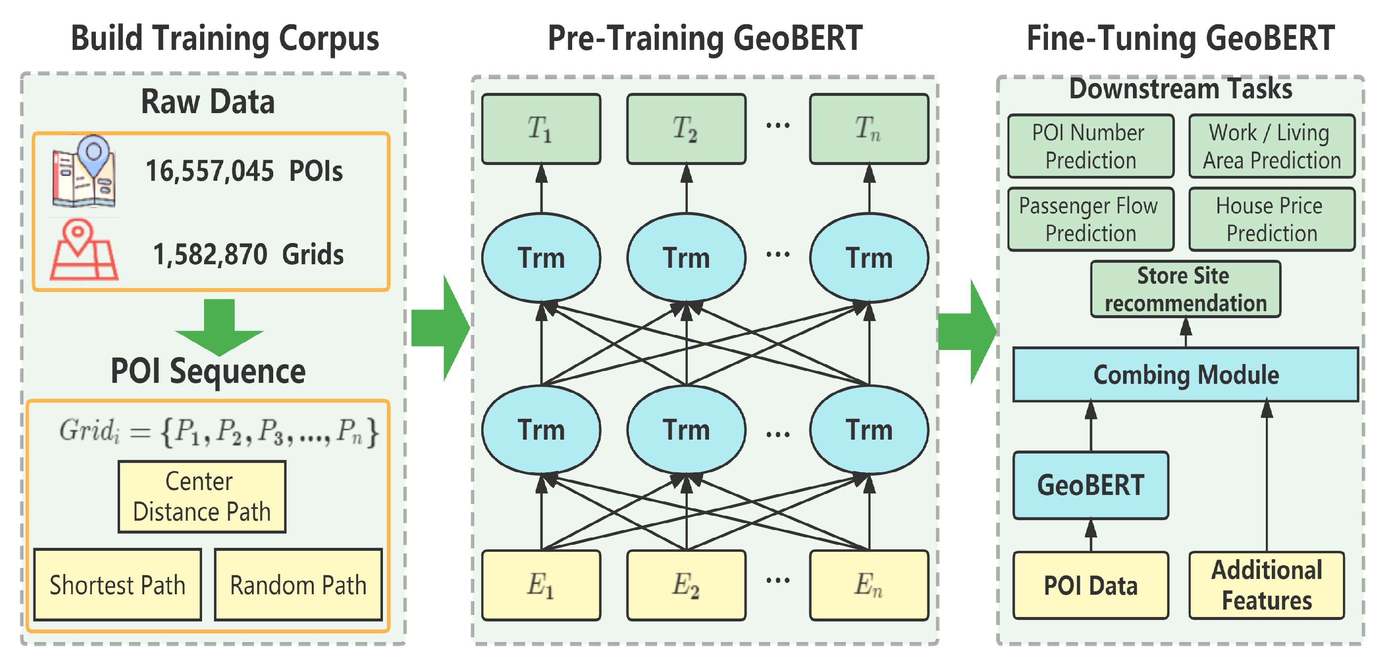
Figure 1 shows the framework of this study. The overall process can be summarized in three modules:
- Build Training Corpus: We collect about 17 million POIs in 30 cities in China and set the level-7 Geohash grid as the basic unit. Taking POI types as tokens and grids as sentences, we build three pre-training corpora based on the “shortest path”, “center distance”, and “random path” methods.
- Pre-Train GeoBERT: Utilizing the BERT structure, we pre-train GeoBERT by masking some percent tokens and then predicting those tokens.
- Fine-tune GeoBERT: GeoBERT is fine-tuned to address five downstream urban tasks. It is worth mentioning that GeoBERT can be used alone or combined with additional features.
3.2. Data and Preprocessing
Most of the corpora of the natural language pre-trained model comes from the Internet and books, where texts are naturally organized. For example, BERT used BooksCorpus (800M words) [41] and English Wikipedia (2500M words). Similarly, POIs are widely available on maps. However, large-scale and high quality text data can be easily acquired while POIs are not. In this study, POI data is collected from AutoNavi, one of China’s most extensive map service providers. We collect around 17 million POIs in the top 30 cities in China by GDP. The POI dataset contains three levels of types, specifically, 11 first-level, 112 s-level, and 214 third-level POI types. In particular, the first-level POI type includes accommodation, enterprise and business, restaurant, shopping, transportation, life services, sport and leisure, science and education, health and medical, government, and public facilities. The percentage of each first-level category is illustrated in Table 1. Each POI has either two or three levels of categories. For example, a coffee shop may have a category hierarchy of “restaurant—coffee shop,” while an Internet cafe may have a category hierarchy of “sport and leisure—entertainment—Internet cafe”. We use the last level of category for unity.
3.3. Basic Geographic Unit
In previous studies, researchers took traffic analysis zone [3] (TAZ), buffer area [5], or other urban functional zone (UFZ) [42] as the basic unit to build a training corpus of POIs. Although this may have more specific practical physical meaning, it is more time-consuming and less effective in the case of the large-scale corpus. Therefore, we use the level-7 Geohash grid as the base unit of POIs, which is easy to retrieve. Moreover, we use a finer-grained grid division, so it can be used for a wider and more refined range of downstream tasks. Geohash (https://en.wikipedia.org/wiki/Geohash, accessed on 30 November 2022) is a public domain geocode system, which encodes a geographic location into a short string of letters and digits. Geohash guarantees that the longer a shared prefix between two geohashes is, the spatially closer together they are. The reverse of this is not guaranteed, as the two points can be very close but have a short or unshared prefix. The area of each level of Geohash is illustrated in Table 2. The max scale is calculated around the equator. In different latitudes, the area will be slightly different. Each level-7 Geohash grid is 153 m × 153 m near the equator. An example of level-7 Geohash grids in Shanghai is shown in Figure 2. In the training corpus, 1,582,870 grids are covered.
3.4. Build Training Corpus
In NLP, words are naturally well-organized according to grammar rules. In a corpus, the sequential order of documents and the contextual relationship between words in each sentence can be used to simulate the contextual relationship of words in real-world human languages. However, POIs are distributed irregularly in urban spaces. In other words, the distribution of POIs is dense in some regions and sparse in others. The spatial distribution of the different types of POI also varies. Thus, we treat each grid analogously as a sentence and the POIs within the grid as words. To obtain a sufficient number of words, we select the last-level categories of POIs as tokens, which is 313 in total. Since the length of the POI sequence (the number of POIs in a grid) is different, we truncate the POI sequence by the max length of 64 and pad short sequences to 64 with 0. The maximum length covers 97.33% situations, as shown in Figure 3. We build our grid-based training corpus on the following three methods:
3.4.1. Shortest Path
The “shortest path” method introduced by Yao et al. [3] constructs a POI sequence based on the Greedy Algorithm. If documents are constructed based on the principle of global optimization, the time cost is exceptionally high, rendering the method unfeasible. However, when dealing with long sequences (e.g., 800+ POIs in a grid), the original shortest path method is still too time-consuming. Therefore, we follow Yao et al.’s idea and improve the algorithm by using a matrix calculation and putting it on a GPU, which significantly reduces the computation time.
The pseudo-code of our shortest path is illustrated in Algorithm 1. Assuming that there are n POIs in a given grid G and denoting , the algorithm returns a sequence L with the shortest path through all POIs. First, we initialize a distance matrix as the Euclidean distance between each pair of POIs <P, P>. We then take the farthest POI pair as the start point and the end point of the path, namely and . At this time, the current path is , and the wait-to-insert set is .
The next task is to keep looking for the correct position and insert the right POI until the set W is empty. The correct position makes the path length shortest under each loop. The pseudo-code of finding correct location and POI is illustrated in Algorithm 2. First, we set up a sub-matrix considering only all possible locations and POIs waiting to be inserted; represent the length of L and W. Suppose that, at the step t+1, POI is inserted between . The path length can be computed as . Specifically, we concat each two adjacent rows in and obtain a 3D matrix () to represent each possible location. There are positions in a sequence of length l. Then, we sum the two adjacent rows to obtain the additional distance. The length reduced when inserting a new POI is calculated as . Finally, we argmin the loss matrix . The correct position index and the POI to be inserted in the next step are obtained.
| Algorithm 1 Shortest Path For POIs In A Grid |
|
| Algorithm 2 Query POI |
|
3.4.2. Center Distance Path
3.4.3. Random Path
To compare with the above two methods, we set up an additional random sequence. The POIs in a grid are randomly sorted into a sequence. The random seed is set to 42.
3.5. Pre-Training GeoBERT
We pre-train the GeoBERT base on the BERT model architecture from Hugging Face (https://huggingface.co/models, accessed on 30 November 2022), utilizing the powerful feature extraction ability of deep bidirectional transformers. Special tokens [CLS] and [SEP] are added at the beginning and end of each sentence, respectively. Input embedding is the sum of token embedding, token type embedding, and position embedding. Following the BERT, we randomly mask some percentage of the input POI-type tokens and then predict those masked tokens. If a token is chosen, it will be replaced by a special token [MASK] for 80% of the time, a random token for 10% of the time, and an original token for 10% of the time. After many attempts, the mask ration of 15% gives the best overall performance.
3.6. Fine-Tuning GeoBERT
In NLP, fine-tuning refers to incrementally training the pre-trained model with a small amount of labelled data. With minimal architectural modification, GeoBERT can be applied to various downstream tasks. We design five geospatial downstream tasks and validate them on the urban data of Shanghai. To better match downstream task indicators, we use the updated POI data. The pre-training POI data was collected in March 2022, while the POI data used in the downstream tasks was collected in September 2022.
3.6.1. POI Number Prediction
The task is to predict the number of POIs in a grid. The number of POIs in a grid reflects the level of socioeconomic activity in the area, and the label can be obtained from the data itself, which makes it suitable for measuring the effect of self-supervised language learning. We choose Shanghai as the study area. After filtering the grids with less than 2 POI, there are a total of 61,521 valid samples. The statistics of the dataset are shown in Table 3, and the visualization is shown in Figure 5.
3.6.2. Work/Living Area Prediction
This task is to predict the function of the grid, that is, whether the current grid functions as a living or working area. Living areas usually have a higher proportion of people living there, while working areas have more people working inside. The division of work and residence areas reflects the city’s current functional zoning and design. Accurate identification of working or living regions is conducive to optimizing urban structure. The statistics of the dataset are shown in Table 4, and the visualization is shown in Figure 6.
3.6.3. Passenger Flow Prediction
The number of visitors on the grid reflects the commercial activity of the current region, which has a high reference value for the location decision of chain stores, advertising, and other marketing activities. Therefore, we design a downstream task to predict the passenger flow on the grid over a period. The passenger flow data is the aggregation of September 2022. The statistics of the dataset are shown in the Table 5, and the visualization is shown in Figure 7.
3.6.4. House Price Prediction
3.6.5. Store Site Recommendation
Location is considered a critical factor in the success of a store in the modern retail industry. Choosing an optimal location to open a new store has always been a headache for brick-and-mortar chain enterprises. We design a site selection recommendation task and take a large chain joint-stock bank as an example. To avoid label leakage, all “bank” tokens are eliminated from the dataset. The statistics of the data set are shown in Table 7. The dataset construction process is shown in Figure 9 below:
- First, there are too little data for just one bank brand in one city, so we use other similar large chain joint-stock banks for data enhancement. Specifically, we select nine other large joint-stock bank brands similar to .
- Second, the grids of normally operating banks of selected brands are taken as positive samples.
- Third, we build the negative samples, which consist of two parts. The first part is the banks of that have already closed in the past. The second part is those non-bank POIs within 500 m of the normally operating banks of .
We set up two experiments. In the first experiment, only POI data is used to fine-tune GeoBERT. In the second one, we use the grid embedding learned by GeoBERT as the basic features and integrate additional grid features to improve the site recommendation task, which is closer to the actual business situation. We calculate about 131 features, which describe the geospatial characteristics of grids in different perspectives. GeoBERT is pre-trained solely on POI data, which can be seen as static information. On the other hand, additional features, such as passenger flow each hour, can provide dynamic information. Limited by space, only some representative features are listed as follows.The summary of primary notations is illustrated in Table 8.
- Passenger flow: Two kinds of features are used to measure the level of passenger flow in a region. First, we calculate the passenger flow of in each hour t of the day. Moreover, we aggregate the eight grids around the current grid as a block to measure the surrounding environment. A block consists of 9 (3*3) adjacent grids. The calculation principle of block features is the same as the grid features but on a larger area (9 grids). See Equation (1). So, we omit the calculation formula of block features in the following features.
- Diversity: We calculate the number of POIs of different categories in each grid to reflect the diversification and heterogeneity of the environment, as shown in Equation (2). is the number of POIs of category c in , is the total number of POIs, and the is the set of all the POI categories. The diversity of block is calculated in the same way.
- Competitiveness: Stores of the same category in a region will form a competitive relationship and influence each other. We define the competitiveness feature in Equation (3). represents the total number of stores of the same category of the target stores in the area around the candidate location j, and is the number of stores of the same category except for the target stores in .
- Traffic Convenience: It reflects the accessibility to different means of transportation (e.g., bus station, subway station, ferry station, etc.), as shown in Equation (4). Here, represents a certain type of transportation, and is the number of all stations of the corresponding transportation type in Gird i.
- Residence: It reflects the surrounding residential conditions. Specifically, it is the number of residential buildings of different grades, for example, ordinary residence, high-grade residence, and villa.
After calculating additional features, we can combine them with GeoBERT. Supposing that the output of the last transformer layer in GeoBERT is h and additional features are x, we calculate the combined embedding in the following four methods:
- Concat: We directly concatenate the output of the transformer layer in GeoBERT and all features before the final classifier layer. There is no additional preprocessing.
- MLP: We put an MLP (Multilayer Perceptron) layer on additional features first and then concatenate it with the transformer before the final classifier layer.
- Weighted: We set a learnable weight matrix for each dimension of additional features and then sum it with transformer outputs before the final classifier layer, where W refers to the weight matrix.
- Gating: We complete a gated summation of transformer outputs and additional features before the final classifier layer, where is a hyper parameter and R is an activation function. Detailed information can be found in the paper [43].
4. Experiments and Results
4.1. Baseline and Setup
4.1.1. Baseline
To the best of our knowledge, GeoBERT is the first large pre-trained model in this field. There are two main types of previous studies. The first is to learn POI-type embedding and aggregate them to grid embedding. The second is supervised learning models in which labels such as land classifications or other business ratios such as sales per square meter are essential. However, we cannot obtain that much labelled data. In brief, there have not been suitable models for comparison. Thus, we compare the most widely used geospatial representation learning model.
- GloVe (2021): Proposed by Zhang et al. [5]. We set the number of POI-type vector dimensions to 70, window size to 10, and epoch to 10, according to the original paper. After training POI-type embedding, we use LightGBM for downstream tasks.
4.1.2. Setup
During the pre-training stage, to compress the space taken up by each sentence and obtain a larger batch size, the maximum sequence length was fixed to 64, which already covers more than 97% of situations. The batch size was set to 256. The hidden size was 768. There were 12 hidden layers and 12 attention heads in each layer. The non-linear activation function was Gelu. The dropout probability for all fully connected layers in the embeddings, encoder, and pooler was set to 0.1. Other parameters were set to default. Detailed information can be found on Hugging Face BertConfig at https://huggingface.co/docs/transformers/model_doc/bert#transformers.BertConfig (accessed on 30 November 2022). We used a single Nvidia A100 40G and pre-trained for 100 epochs. The Python version was 3.8.11, and the CUDA version was 11.6. The deep learning framework was PyTorch. Training GeoBERT from scratch on our corpus took about two days. During the fine-tuning period, we put one MLP layer after the output of the last hidden layer in GeoBERT and applied a dropout of 0.1. We fine-tuned GeoBERT for two to five epochs using a batch size of 32 and selected the best results. For regression tasks, we used MSE (mean square error) and MAE(mean absolute error) to evaluate, while F1-score and Accuracy were used for classification tasks. For regression tasks, the lower the indicator, the better. For classification tasks, the higher the indicator, the better. In all fine-tuning datasets, we used 80% for training and 20% for testing under the random seed of 42.
4.2. Downstream Task Results
- POI Number Prediction:The POI number prediction experiment result illustrated in Table 9 shows that GeoBERT significantly outperformed Word2vec and GloVe in three different training corpora. Generally, the overall performance of Word2vec was better than GloVe, while GeoBERT pre-trained on the shortest path corpus achieved the best result (0.1790 in MSE and 0.1343 in MAE).
- Working∖Living Area Prediction:The result of work and living area prediction is illustrated in Table 10. The GeoBERT series outperformed the series of Word2vec and GloVe, and GeoBERT pre-trained on random sequence corpus obtained the best results, with Accuracy of 0.7739 and F1-score 0.7719. However, the difference between groups and within groups was small. The best model GeoBERT-RandomPath improved the worst model by 4.91% in Accuracy and by 8.83% in F1-score.
- Passenger Flow Prediction: As exhibited in Table 11, the results in GeoBERT on passenger flow prediction far exceeded Word2vec and GloVe. GeoBERT pre-trained on the shortest path corpus obtained the best results, with 0.1446 in MSE and 0.1809 in MAE. The difference between the three corpora was not quite significant.
- House Price Prediction: As depicted in Table 12, GeoBERT significantly outperformed the other two models, and the performance difference between these three models was substantial. GeoBERT pre-trained on the shortest path obtained the best result.
- Store Site Recommendation: The results of store site recommendation with POIs only are shown in Table 13. GeoBERT achieved better performance, while GeoBERT pre-trained on center distance corpus obtained the best result, with 0.8359 in Accuracy and 0.7922 in F1-score. The differences between the three GeoBERT models are not considerable. The results of store site recommendation with additional features are illustrated in Table 14. We can see that with additional features, both Accuracy and F1-score were improved in all cases. Among different combination methods, the MLP method obtained the best performance, increasing Accuracy by 2.45% and F1-score by 3.04%. The result of these two experiments illustrate the following points:
- GeoBERT obtains good grid embedding from POI data and can be directly used for store site recommendation.
- GeoBERT is scalable and can be jointly used with additional features. The effect will be improved if more dimensional data is provided.
GeoBERT was pre-trained solely on POI data, which can be seen as static urban information. On the other hand, additional features, such as passenger flow each hour, can provide dynamic ubran information. However, in practice, additional features, such as user profiles and passenger flow data, are hard to access and often subject to privacy restrictions, while POIs are not. Therefore, GeoBERT alone can be used to achieve pretty good results which proves that GeoBERT has practical applied value. To sum up, POI data is the most readily available urban data that can contain much geospatial information. However, other features can also add information from different dimensions, especially user consumption behavior and travel behavior. GeoBERT is effective and having additional features would be better for more specific tasks.
5. Discussion
5.1. Result on Downstream Tasks
We can find out that GeoBERT outperforms Word2vec and GloVe on all five downstream tasks, which proves that pre-training on large corpora helps extract the geospatial information of POIs. However, the performance of these three models on different tasks is different. On classification tasks, Word2vec and GloVe are still competitive, which is illustrated in Figure 10. For example, in the working∖living area prediction task, GeoBERT only exceeds the best Word2vec model by 1.5% in Accuracy and 3.82% in F1-score, while in regression tasks, GeoBERT is substantially superior to Word2vec and GloVe, as shown in Figure 11. The difference illustrates that GeoBERT learned more accurate representation of grids and is more capable of fine-grained tasks.
Another interesting finding is about the different training corpora. Among the three training corpora, GeoBERT pre-trained on the shortest path gives better results in general. However, this is not absolute; for example, GeoBERT-CenterDistance gives the best store site recommendation result. The same conclusion can also be drawn for the other two models. Actually, previous studies have neglected to compare different POI sequences. The results of five downstream tasks show that the differences between the three corpora are small, which means the precise context relationship between POIs in a certain area (e.g., a level-7 Geohash grid) does not play a critical role. It is an interesting finding, and we will discuss it further later.
5.2. Ablation Study
Section 3.5 mentions that GeoBERT uses 15% as the masking ratio during the pre-training stage. The following is an ablation study to evaluate the effect of different masking strategies on the passenger flow prediction task. All the models were pre-trained for 40 epochs to save computing resources and time. We tested the masking ratio for 15%, 30%, 50%, and 70%. From Table 15, it can be seen that GeoBERT is highly robust to different masking strategies, and overall, 15% performs the best.
5.3. What Does GeoBERT Actually Learn?—Part 1: Distilling Common Patterns
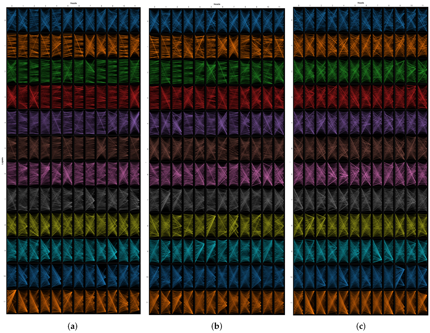
In order to determine what GeoBERT learns and the difference between the three kinds of POI sequences, we delve into the self-attention mechanism. GeoBERT, following the original BERT model, uses 12 layers with 12 attention heads in each layer. Therefore, there are 144 (12 × 12) different attention mechanisms in total in which is difficult to intuit the meaning of its learned weights in such complexity. Fortunately, with the help of attention visualization tools [45], we can explore the attention patterns of various layers and heads and analyse the underlying principles involved.
We select a grid with 22 POIs for demonstration purposes. The POI sequences of the three versions are shown in Table 16. The model views of the three different GeoBERT models are illustrated in Figure 11. Each has 12 layers and 12 attention heads in each layer.
5.3.1. Pattern 1: Attention to Next Token
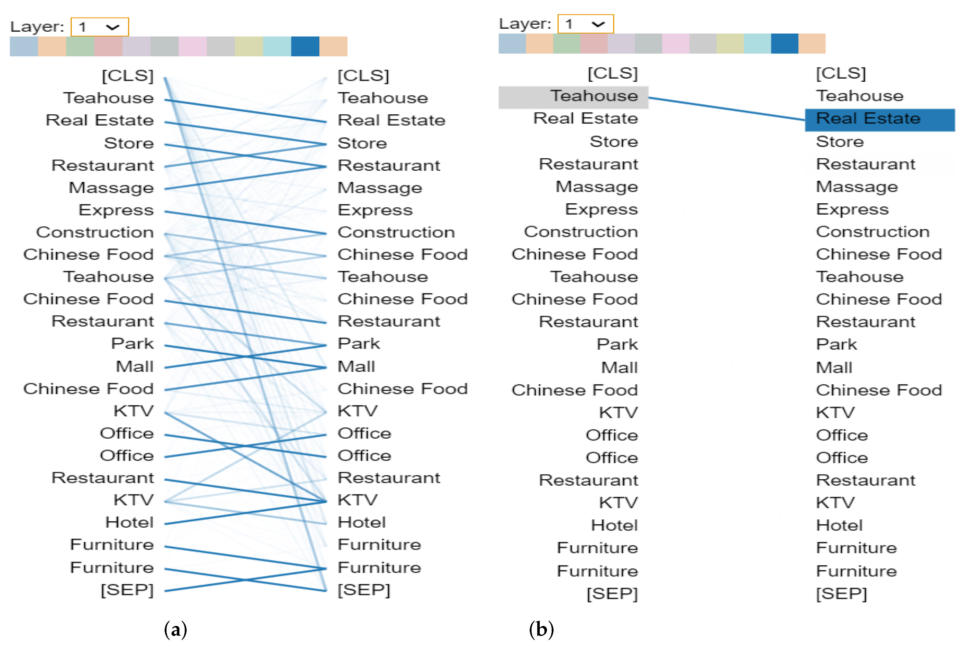
Like BERT, most of the attention at a particular position is directed to the next token in the sequence. Figure 12 is an example of GeoBERT-ShortestPath for Layer 1, Head 10. Figure 12a on the left shows the attention for all tokens in a grid, while Figure 12b on the right shows a specific token “Teahouse”, which is directed to the next token “Real Estate”. This pattern is considered to be related to the backward RNN, where state updates are made sequentially from right to left.
5.3.2. Pattern 2: Attention to Previous Token
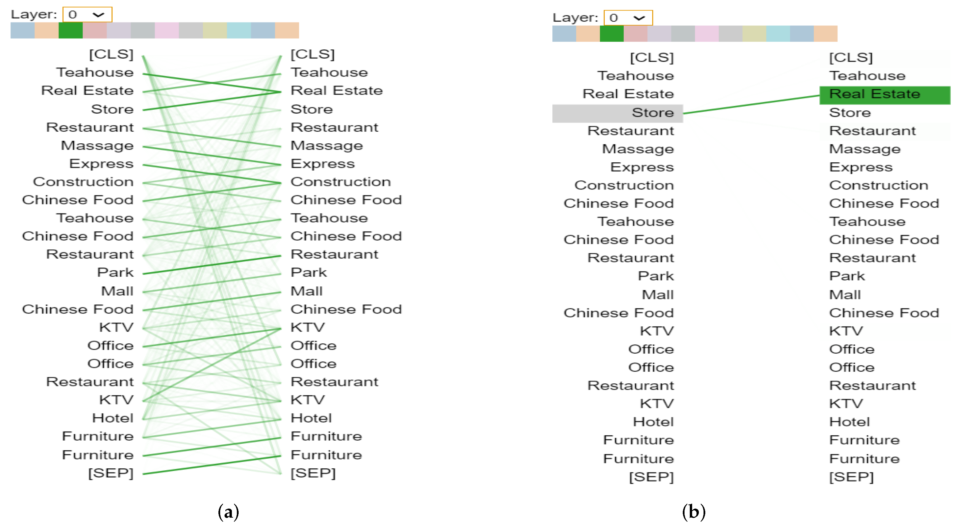
In this pattern, much attention is directed to the previous token in the sentence. We still take the shortest Path POI sequence in Table 16 as an example. The attention mechanism in GeoBERT-ShortestPath of Layer 0, Head 2, is illustrated in Figure 13. We can find that most of the attention for “Store” is related to “Real Estate”. Like Pattern 1, this is loosely related to a sequential RNN, in this case, the forward RNN.
5.3.3. Pattern 3: Long-Distance Dependencies
In this pattern, many attention heads tend to have a long-distance dependency. In particular, attention is paid to identical or related words, including the source word itself. This pattern is also exhibited in the appendix of the original Transforms [28]. Figure 14 listed below is Layer 6 in GeoBERT-ShortestPath. Most of the attention for the token “Real Estate” is directed to itself and “Express”. This pattern is not so distinct, with attention dispersed over many different words in other heads, which can be seen from the different colors in the right sequence in Figure 14b.
5.4. What Does GeoBERT Actually Learn?—Part2: Deeper Insights
In Section 5.3, we explore the three common patterns learned by GeoBERT from the perspective of self-attentions. The above findings explain part of the rationale behind GeoBERT, but they still require further research. In Part 2, we will drill deeper into GeoBERT’s attention mechanism and reveal the answer to two key questions.
5.4.1. Question 1: What Is the Difference between the Three POI Sequence Construction Methods?
In Section 3.4, we proposed three different POI sequence construction methods and pre-trained three GeoBERT models on them. Previous studies have proven these construction methods (Shortest Path and Center Distance Path) effective in extracting POI location information. To date, no study has compared these methods and analyzed the spatial information in depth in the POI sequences. With the help of Transformer structure’s powerful information extraction capabilities, we can further explore the difference between these construction methods and what GeoBERT has learned.
In brief, there is a contextual relationship but no exact back-and-forth relationship among adjacent POIs in a grid, and GeoBERT can learn this kind of location information in shallow attention layers. We illustrate the attention mechanism of Layer 1 and Layer 2 for GeoBERT-ShortestPath, GeoBERT-CenterDistance, and GeoBERT-RandomPath in Figure 15, Figure 16 and Figure 17, respectively. From Layer 1 and Layer 2 of GeoBERT-ShortestPath (Figure 15) and GeoBERT-CenterDistance (Figure 16), we can intuitively find that there are higher attention weights between a token and the two adjacent tokens, presented as pairs of crossed straight lines in the image, while in the GeoBERT-RandomPath (Figure 17), the same phenomenon has not been observed. The above findings indicate two things. The first is that attention Layers 1 and 2 of the GeoBERT can learn the adjacency relationship between POIs. The second is that in terms of how the POIs are organized, both the shortest path and the center distance path contain location information, but random sequences cannot, which is in line with expectations. On the other hand, the pairs of cross lines between adjacent tokens show that POIs have close context relationships but do not have strict back-and-forth ones such as natural language, which has more specific grammar and syntax rules.
5.4.2. Question 2: Why Do the Three Models Have Similar Effects on All Five Downstream Tasks?
Section 5.1 compared the GeoBERT models pre-trained on three different corpora. Results on downstream tasks show that although GeoBERT-ShortestPath achieves the overall best performance, the difference between the three models is not as significant as expected. In this section, we try to answer why these three models perform similarly since they are pre-trained on different POI sequences.
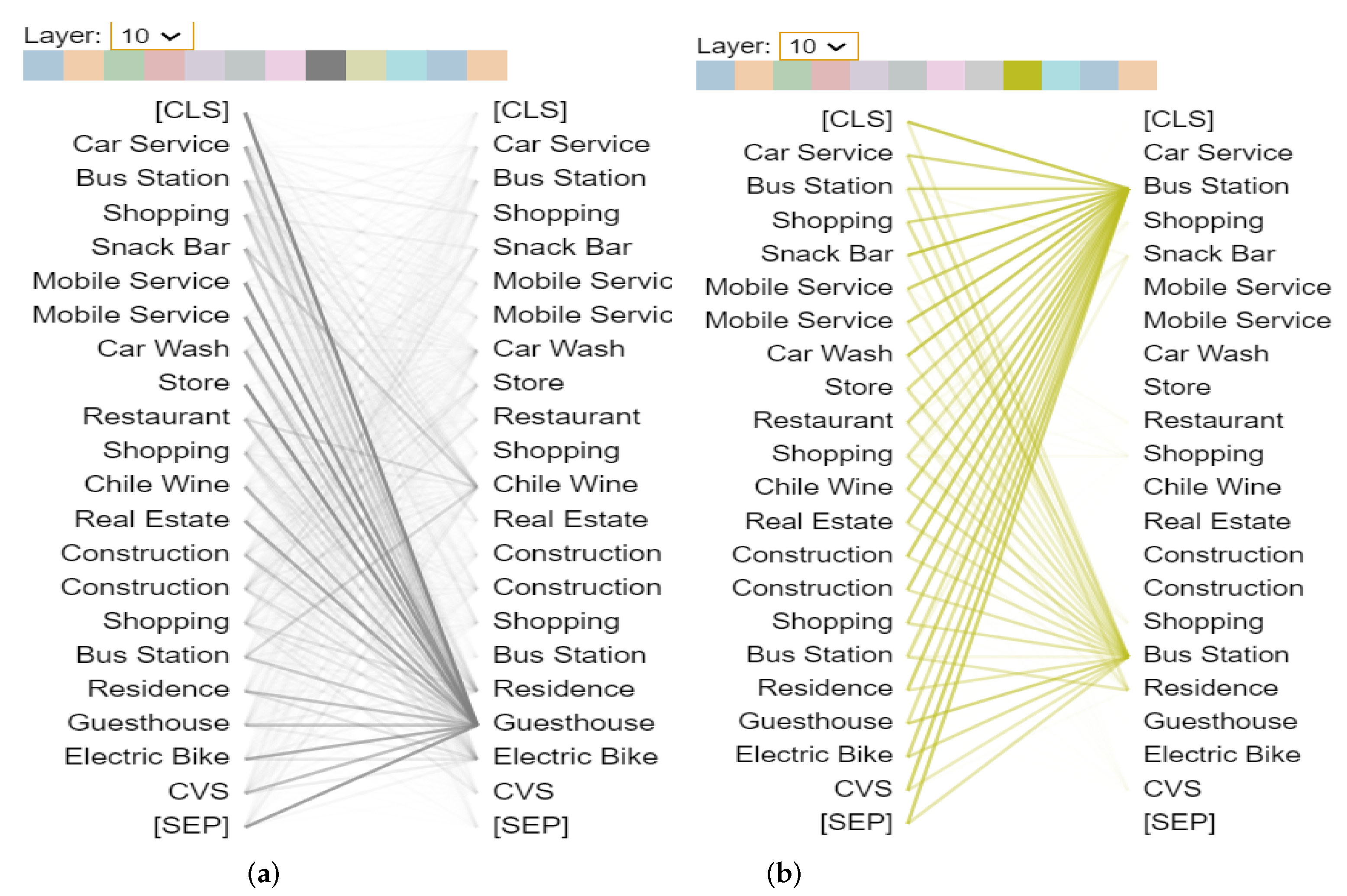
From the previous question, we know that Center Distance Corpus and Shortest Path Corpus contain the location information and can be learned by GeoBERT, while Random Path does not. However, GeoBERT-RandomPath is still competitive, which is worth further exploration. In our opinion, what matters is not the sequence order of POIs in a grid but the co-occurrence between POIs. However, the sequence knowledge learned by GeoBERT helps the model perform better in fine-grained tasks, which explains that GeoBert-RandomPath performs the worst in regression tasks. (See Table 9, Table 11 and Table 12). What is more important is that GeoBERT can capture the co-occurrence between POIs and recognize specific tokens that have more significance in a grid. In other words, the core ability of GeoBERT is to find the several tokens that play the most critical roles in downstream tasks. Moreover, this ability is acquired in deeper attention layers. Refer to Figure 11 for the visualization of all layers and heads.
Figure 18 shows Layer 9, Head 9, and Layer 10, Head 8 in GeoBERT-ShortestPath, where most tokens have attention weights to token “Departments Store” and token “Hotel”. Thus, we perceive that these two tokens play a more critical role. We call these kinds of tokens the “anchor POIs” of a grid. To some extent, these POIs can represent the grid. It is worth noting that there is not just one such token. In most cases, there are multiple ones in different layers and heads representing different attributes. Figure 19 exhibits the three models’ attention Layer 10 (with all heads). It can be determined that tokens “Mall” and “Hotel” attract the most attention in all cases despite their different locations in the sequence. This finding also supports our conclusion on the issue of the core ability of GeoBERT. In addition to this case in Table 16, we list two additional cases in Figure 20 and Figure 21. The same conclusion can be drawn.
6. Conclusions and Future Work
6.1. Conclusions
This paper proposes the first pre-trained geospatial representation learning model called GeoBERT based on POI data and a BERT Model. We collected 17 million POIs and constructed different POI sequences for each level-7 Geohash grid. The sequence is built on three methods: the shortest path, the center distance path, and the random path. After pre-training, GeoBERT was fine-tuned on five downstream tasks. Compared with other NLP models (Word2vec, GloVe) used in this field, GeoBERT obtained the highest results on all five tasks. Moreover, GeoBERT is highly scalable. Combining the grid embedding learned from GeoBERT with additional features can further improve the performance. Then, we went deep into the attention mechanism in the GeoBERT and analyzed what GeoBERT actually learns. Through detailed visualization analysis, we reached three main conclusions.
- The shortest path and center distance contain the position information among POIs in a grid, while the random path method does not.
- GeoBERT learns the position information in the shallow attention layers. In deep attention layers, GeoBERT captures co-occurrence among POIs and identifies the most important POIs, called the anchor POIs in a grid.
- The sequential relationship between POIs does not play an important role. What matters is the co-occurrence among POIs and the specific anchor POIs learned in deep attention layers.
6.2. Future Work
The above conclusions guide our subsequent work. Since different POI sequences have limited effect on the experimental results, we intend to take POIs in a grid as 2D raster data rather than construct a POI sequence for future work. A grid with POIs can be seen as an image to some extent. The difficulty, however, is how to process the 2D POI data as an image and encode it into vectors. From another point of view, we can further optimize our work in the future by incorporating POI data with satellite images, making it a multi-modal pre-training model. A simple and straight way is to take POI as text and satellite as image. By doing this, we can learn more information about a grid and make the model capable of more tasks.
Author Contributions
Conceptualization, Y.G. and H.W.; methodology, Y.G. and Y.X.; formal analysis, Y.G. and S.W.; supervision, H.W. and Y.X.; writing—original draft preparation, Y.G. and S.W.; writing—review and editing, H.W. and Y.X.; All authors have read and agreed to the published version of the manuscript.
Funding
This research was supported by the National Nature Science Foundation of China (Grant No. 62176185), and the Top Discipline Plan of Shanghai Universities-Class I (Grant No. 2022-3-YB-02).
Data Availability Statement
POI data can be accessed by AutoNavi API at https://developer.amap.com/api/webservice/guide/api/search/ (accessed on 1 June 2022). POI number data and store site recommendation data can be acquired from POI dataset itself. Data used in fine-tuning is provided by ayz.ai at http://www.wayz.ai/ (accessed on 1 June 2022). Restrictions apply to the availability of the data (e.g., passenger flow data and working/living data), which is used under license for this study.
Acknowledgments
The authors would like to thank the Wayz.ai for providing data and experiment facilities used in this study.
Conflicts of Interest
The authors declare no conflict of interest.
References
- Yao, Z.; Fu, Y.; Liu, B.; Hu, W.; Xiong, H. Representing urban functions through zone embedding with human mobility patterns. In Proceedings of the Twenty-Seventh International Joint Conference on Artificial Intelligence (IJCAI-18), Stockholm, Sweden, 13–19 July 2018. [Google Scholar]
- Huang, C.; Zhang, J.; Zheng, Y.; Chawla, N.V. DeepCrime: Attentive hierarchical recurrent networks for crime prediction. In Proceedings of the 27th ACM International Conference on Information and Knowledge Management, Turin, Italy, 22–26 October 2018; pp. 1423–1432. [Google Scholar]
- Yao, Y.; Li, X.; Liu, X.; Liu, P.; Liang, Z.; Zhang, J.; Mai, K. Sensing spatial distribution of urban land use by integrating points-of-interest and Google Word2Vec model. Int. J. Geogr. Inf. Sci. 2017, 31, 825–848. [Google Scholar] [CrossRef]
- Niu, H.; Silva, E.A. Delineating urban functional use from points of interest data with neural network embedding: A case study in Greater London. Comput. Environ. Urban Syst. 2021, 88, 101651. [Google Scholar] [CrossRef]
- Zhang, C.; Xu, L.; Yan, Z.; Wu, S. A glove-based poi type embedding model for extracting and identifying urban functional regions. ISPRS Int. J. Geo-Inf. 2021, 10, 372. [Google Scholar] [CrossRef]
- Yan, B.; Janowicz, K.; Mai, G.; Gao, S. From itdl to place2vec: Reasoning about place type similarity and relatedness by learning embeddings from augmented spatial contexts. In Proceedings of the 25th ACM SIGSPATIAL International Conference on Advances in Geographic Information Systems, Redondo Beach, CA, USA, 7–10 November 2017; pp. 1–10. [Google Scholar]
- Devlin, J.; Chang, M.W.; Lee, K.; Toutanova, K. BERT: Pre-training of Deep Bidirectional Transformers for Language Understanding. arXiv 2018, arXiv:1810.04805. [Google Scholar]
- Radford, A.; Narasimhan, K.; Salimans, T.; Sutskever, I. Improving Language Understanding by Generative Pre-Training. 2018. Available online: https://www.cs.ubc.ca/~amuham01/LING530/papers/radford2018improving.pdf (accessed on 23 November 2022).
- Mai, G.; Janowicz, K.; Hu, Y.; Gao, S.; Yan, B.; Zhu, R.; Cai, L.; Lao, N. A review of location encoding for GeoAI: Methods and applications. Int. J. Geogr. Inf. Sci. 2022, 36, 639–673. [Google Scholar] [CrossRef]
- Yuan, J.; Zheng, Y.; Xie, X. Discovering regions of different functions in a city using human mobility and POIs. In Proceedings of the 18th ACM SIGKDD International Conference on Knowledge Discovery and Data Mining, Beijing, China, 12–16 August 2012; pp. 186–194. [Google Scholar]
- Gao, S.; Janowicz, K.; Couclelis, H. Extracting urban functional regions from points of interest and human activities on location-based social networks. Trans. GIS 2017, 21, 446–467. [Google Scholar] [CrossRef]
- Mikolov, T.; Sutskever, I.; Chen, K.; Corrado, G.S.; Dean, J. Distributed representations of words and phrases and their compositionality. Adv. Neural Inf. Process. Syst. 2013, 26. [Google Scholar]
- Feng, S.; Cong, G.; An, B.; Chee, Y.M. Poi2vec: Geographical latent representation for predicting future visitors. In Proceedings of the Thirty-First AAAI Conference on Artificial Intelligence, San Francisco, CA, USA, 4–9 February 2017. [Google Scholar]
- Xiang, M. Region2vec: An Approach for Urban Land Use Detection by Fusing Multiple Features. In Proceedings of the 2020 6th International Conference on Computing and Artificial Intelligence, Tianjin, China, 17–20 October 2020; pp. 13–18. [Google Scholar] [CrossRef]
- Zhu, M.; Wei, C.; Xia, J.; Ma, Y.; Zhang, Y. Location2vec: A Situation-Aware Representation for Visual Exploration of Urban Locations. IEEE Trans. Intell. Transp. Syst. 2019, 20, 3981–3990. [Google Scholar] [CrossRef]
- Sun, Z.; Jiao, H.; Wu, H.; Peng, Z.; Liu, L. Block2vec: An Approach for Identifying Urban Functional Regions by Integrating Sentence Embedding Model and Points of Interest. ISPRS Int. J. Geo-Inf. 2021, 10, 339. [Google Scholar] [CrossRef]
- Zhang, J.; Li, X.; Yao, Y.; Hong, Y.; He, J.; Jiang, Z.; Sun, J. The Traj2Vec model to quantify residents’ spatial trajectories and estimate the proportions of urban land-use types. Int. J. Geogr. Inf. Sci. 2021, 35, 193–211. [Google Scholar] [CrossRef]
- Shoji, Y.; Takahashi, K.; Dürst, M.J.; Yamamoto, Y.; Ohshima, H. Location2vec: Generating distributed representation of location by using geo-tagged microblog posts. In Proceedings of the International Conference on Social Informatics, Saint-Petersburg, Russia, 25–28 September 2018; pp. 261–270. [Google Scholar]
- Zhang, Y.; Li, Q.; Tu, W.; Mai, K.; Yao, Y.; Chen, Y. Functional urban land use recognition integrating multi-source geospatial data and cross-correlations. Comput. Environ. Urban Syst. 2019, 78, 101374. [Google Scholar] [CrossRef]
- McKenzie, G.; Adams, B. A data-driven approach to exploring similarities of tourist attractions through online reviews. J. Locat. Based Serv. 2018, 12, 94–118. [Google Scholar] [CrossRef]
- Zhang, Y.; Zheng, X.; Helbich, M.; Chen, N.; Chen, Z. City2vec: Urban knowledge discovery based on population mobile network. Sustain. Cities Soc. 2022, 85, 104000. [Google Scholar] [CrossRef]
- Huang, W.; Cui, L.; Chen, M.; Zhang, D.; Yao, Y. Estimating urban functional distributions with semantics preserved POI embedding. Int. J. Geogr. Inf. Sci. 2022, 36, 1–26. [Google Scholar] [CrossRef]
- Liu, Y.; Ott, M.; Goyal, N.; Du, J.; Joshi, M.; Chen, D.; Levy, O.; Lewis, M.; Zettlemoyer, L.; Stoyanov, V. Roberta: A robustly optimized bert pretraining approach. arXiv 2019, arXiv:1907.11692. [Google Scholar]
- Yang, Z.; Dai, Z.; Yang, Y.; Carbonell, J.; Salakhutdinov, R.R.; Le, Q.V. Xlnet: Generalized autoregressive pretraining for language understanding. Adv. Neural Inf. Process. Syst. 2019, 32. [Google Scholar]
- Lan, Z.; Chen, M.; Goodman, S.; Gimpel, K.; Sharma, P.; Soricut, R. Albert: A lite bert for self-supervised learning of language representations. arXiv 2019, arXiv:1909.11942. [Google Scholar]
- Brown, T.; Mann, B.; Ryder, N.; Subbiah, M.; Kaplan, J.D.; Dhariwal, P.; Neelakantan, A.; Shyam, P.; Sastry, G.; Askell, A.; et al. Language models are few-shot learners. Adv. Neural Inf. Process. Syst. 2020, 33, 1877–1901. [Google Scholar]
- Han, X.; Zhang, Z.; Ding, N.; Gu, Y.; Liu, X.; Huo, Y.; Qiu, J.; Yao, Y.; Zhang, A.; Zhang, L.; et al. Pre-trained models: Past, present and future. AI Open 2021, 2, 225–250. [Google Scholar] [CrossRef]
- Vaswani, A.; Shazeer, N.; Parmar, N.; Uszkoreit, J.; Jones, L.; Gomez, A.N.; Kaiser, Ł.; Polosukhin, I. Attention is all you need. Adv. Neural Inf. Process. Syst. 2017, 30, 6000–6010. [Google Scholar]
- Dosovitskiy, A.; Beyer, L.; Kolesnikov, A.; Weissenborn, D.; Zhai, X.; Unterthiner, T.; Dehghani, M.; Minderer, M.; Heigold, G.; Gelly, S.; et al. An image is worth 16x16 words: Transformers for image recognition at scale. arXiv 2020, arXiv:2010.11929. [Google Scholar]
- He, K.; Chen, X.; Xie, S.; Li, Y.; Dollár, P.; Girshick, R. Masked autoencoders are scalable vision learners. In Proceedings of the IEEE/CVF Conference on Computer Vision and Pattern Recognition, New Orleans, LA, USA, 19–20 June 2022; pp. 16000–16009. [Google Scholar]
- Bao, H.; Dong, L.; Wei, F. Beit: Bert pre-training of image transformers. arXiv 2021, arXiv:2106.08254. [Google Scholar]
- Alsentzer, E.; Murphy, J.R.; Boag, W.; Weng, W.H.; Jin, D.; Naumann, T.; McDermott, M. Publicly available clinical BERT embeddings. arXiv 2019, arXiv:1904.03323. [Google Scholar]
- Huang, K.; Altosaar, J.; Ranganath, R. Clinicalbert: Modeling clinical notes and predicting hospital readmission. arXiv 2019, arXiv:1904.05342. [Google Scholar]
- Fang, X.; Liu, L.; Lei, J.; He, D.; Zhang, S.; Zhou, J.; Wang, F.; Wu, H.; Wang, H. Geometry-enhanced molecular representation learning for property prediction. Nat. Mach. Intell. 2022, 4, 127–134. [Google Scholar] [CrossRef]
- Gu, Y.; Tinn, R.; Cheng, H.; Lucas, M.; Usuyama, N.; Liu, X.; Naumann, T.; Gao, J.; Poon, H. Domain-specific language model pretraining for biomedical natural language processing. ACM Trans. Comput. Healthc. 2021, 3, 1–23. [Google Scholar] [CrossRef]
- Lee, J.; Yoon, W.; Kim, S.; Kim, D.; Kim, S.; So, C.H.; Kang, J. BioBERT: A pre-trained biomedical language representation model for biomedical text mining. Bioinformatics 2020, 36, 1234–1240. [Google Scholar] [CrossRef] [Green Version]
- Beltagy, I.; Lo, K.; Cohan, A. SciBERT: A pretrained language model for scientific text. arXiv 2019, arXiv:1903.10676. [Google Scholar]
- Liu, X.; Yin, D.; Zhang, X.; Su, K.; Wu, K.; Yang, H.; Tang, J. Oag-bert: Pre-train heterogeneous entity-augmented academic language models. arXiv 2021, arXiv:2103.02410. [Google Scholar]
- Huang, J.; Wang, H.; Sun, Y.; Shi, Y.; Huang, Z.; Zhuo, A.; Feng, S. ERNIE-GeoL: A Geography-and-Language Pre-trained Model and its Applications in Baidu Maps. In Proceedings of the 28th ACM SIGKDD Conference on Knowledge Discovery and Data Mining, Washington, DC, USA, 14–18 August 2022; pp. 3029–3039. [Google Scholar]
- Zhou, J.; Gou, S.; Hu, R.; Zhang, D.; Xu, J.; Jiang, A.; Li, Y.; Xiong, H. A collaborative learning framework to tag refinement for points of interest. In Proceedings of the 25th ACM SIGKDD International Conference on Knowledge Discovery & Data Mining, San Diego, CA, USA, 15–18 August 2019; pp. 1752–1761. [Google Scholar]
- Zhu, Y.; Kiros, R.; Zemel, R.; Salakhutdinov, R.; Urtasun, R.; Torralba, A.; Fidler, S. Aligning books and movies: Towards story-like visual explanations by watching movies and reading books. In Proceedings of the IEEE International Conference on Computer Vision, Santiago, Chile, 7–13 December 2015; pp. 19–27. [Google Scholar]
- Lu, W.; Tao, C.; Li, H.; Qi, J.; Li, Y. A unified deep learning framework for urban functional zone extraction based on multi-source heterogeneous data. Remote Sens. Environ. 2022, 270, 112830. [Google Scholar] [CrossRef]
- Rahman, W.; Hasan, M.K.; Lee, S.; Zadeh, A.; Mao, C.; Morency, L.P.; Hoque, E. Integrating multimodal information in large pretrained transformers. NIH Public Access 2020, 2020, 2359. [Google Scholar]
- Ke, G.; Meng, Q.; Finley, T.; Wang, T.; Chen, W.; Ma, W.; Ye, Q.; Liu, T.Y. Lightgbm: A highly efficient gradient boosting decision tree. Adv. Neural Inf. Process. Syst. 2017, 30. [Google Scholar]
- Vig, J. A Multiscale Visualization of Attention in the Transformer Model. In Proceedings of the 57th Annual Meeting of the Association for Computational Linguistics: System Demonstrations, Florence, Italy, 28 July–2 August 2019; pp. 37–42. [Google Scholar] [CrossRef]
Figure 1.
The overall framework of this study consists of three parts. The part on the left side shows how we construct pre-training corpora based on POIs and Geohash Grids. The middle part shows the model structure, which is based on the BERT structure. E represents the input embedding, Trm refers to a transformer block, and T represents the output token. On the right side is the fine-tuning module. We design five practical downstream tasks. The grid embedding learned from GeoBERT can be directly used for fine-tuning or combined with other features.

Figure 2.
The left part exhibits the area of Shanghai, which covers 404,697 level-7 Geohash grids in total. On the right, is a slice that covers 20 grids. Each level-7 grid can be represented by a unique Geohash string of length 7. All the smaller grids that belong to the same larger grid of the upper level share the same prefix. As shown in the figure, the Geohash of 4 grids in the lower right corner share six characters “wtw3w3” in the prefix since they all belong to a much larger level-6 Geohash grid. The same phenomenon can be observed in all four corners.

Figure 3.
Distribution of POI sequence length of grids. The POI sequence length is the number of POIs in a level-7 Geohash grid. The max length is set to 64, which covers 97.33%.
Figure 3.
Distribution of POI sequence length of grids. The POI sequence length is the number of POIs in a level-7 Geohash grid. The max length is set to 64, which covers 97.33%.

Figure 4.
Construct a POI sequence based on distance ordering from the center point.

Figure 5.
The POI number dataset of Shanghai.

Figure 6.
The working/living area dataset of Shanghai, where yellow refers to living area and red to working area.
Figure 6.
The working/living area dataset of Shanghai, where yellow refers to living area and red to working area.

Figure 7.
The passenger flow dataset of Shanghai, where red refers to high-density areas.

Figure 8.
The house price dataset of Shanghai, where red refers to higher house prices.

Figure 9.
The process of building a bank recommendation dataset.

Figure 10.
Results of classification tasks. Word2vec and GloVe still achieve good results. GeoBERT leads Word2vec by 4.49% in Accuracy for the store site recommendation task and 1.51% for the working∖living area prediction task.
Figure 10.
Results of classification tasks. Word2vec and GloVe still achieve good results. GeoBERT leads Word2vec by 4.49% in Accuracy for the store site recommendation task and 1.51% for the working∖living area prediction task.

Figure 11.
Self-attention mechanism in GeoBERT. GeoBERT consists of 12 layers and 12 heads in each layer. Each row represents a layer (from 0 to 11). Each block represents a head (from 0 to 11). The lines between pairs of tokens in a head show the self-attention weights between them. The darker the color is, the greater the weight between the two tokens. Different layers are represented by different colors, while the same color represents heads in the same layer. These are better viewed in color: (a) GeoBERT-ShortestPath; (b) GeoBERT-CenterDistance; (c) GeoBERT-RandomPath.

Figure 12.
The pattern of attention to the next token. The attention mechanism for shortest Path POI sequence example in Table 16 is illustrated. Note that the index starts at 0. Most tokens have a heavy attention weight directed to the subsequent tokens. However, this pattern is not absolute since we can see that some tokens are directed to the other tokens. Colors on the top identify the corresponding attention head(s), while the depth of color reflects the attention score: (a) attention weights for all tokens in Layer 1, Head 10; (b) attention weights for selected token ’Teahouse’.

Figure 13.
The pattern of attention to the previous token. In the example of Layer 0, Head 2, most tokens show apparent attention weight directed to the previous tokens. Of course, there are some exceptions, such as the token “Teahouse”, which still has close attention to the next token “Real Estate”: (a) attention weights for all tokens in Layer 0, Head 2; (b) attention weights for selected token ’Store’.

Figure 14.
Pattern of long-distance dependencies. “Real Estate” is directed to itself and “Express” in (a). However, the attention is also dispersed over many different words which can be seen in (b). The color in the right sequence represents its corresponding head with yellow for Head 1 and green for Head 2: (a) attention weights for selected token “Real Estate” in Layer 6, Head 1; (b) attention weights for selected token “Real Estate” in Layer 6, heads 1 (orange) and 2 (green).

Figure 15.
Attention Layer 1 and Layer 2 in GeoBERT-ShortestPath. We can see pairs of cross lines between adjacent tokens, which means that GeoBERT has learned the position information between adjacent tokens. (a) Attention Layer 1; (b) Attention Layer 2.
Figure 15.
Attention Layer 1 and Layer 2 in GeoBERT-ShortestPath. We can see pairs of cross lines between adjacent tokens, which means that GeoBERT has learned the position information between adjacent tokens. (a) Attention Layer 1; (b) Attention Layer 2.

Figure 16.
Attention Layer 1 and Layer 2 in GeoBERT-CenterDistance. Pairs of cross lines between adjacent tokens can be clearly observed, and the conclusion is similar to the shortest Path. Moreover, most of these signs occur at shallow attention layers, basically from Layer 0 to Layer 2. Thus, we believe that in the shallow attention layers, GeoBERT learns the position information among POIs: (a) Attention Layer 1; (b) Attention Layer 2.

Figure 17.
Attention Layer 1 and Layer 2 in GeoBERT-RandomPath. Unlike the above two methods, there were no obvious signs observed. Therefore, we think that no position information has been acquired by GeoBERT-RandomPath. This phenomenon is reasonable since all POIs are ordered randomly: (a) Attention Layer 1: (b) Attention Layer 2.

Figure 18.
Two specific attention heads in GeoBERT-ShortestPath. In both figures, tokens “Mall” and “Hotel” strongly connect with all other tokens. We define this kind of token as the “Anchor POIs” in a grid. Anchor POIs play essential roles in a grid and to some extent can represent certain attributes of the whole grid: (a) Layer 9, Head 9; (b) Layer 10, Head 8.

Figure 19.
Attention Layer 10 (with all heads) of three models. Although “Mall’ and “Hotel” are in different positions in different corpora, they are successfully recognized by the models. As we have mentioned, the core ability of GeoBERT is to identify the most significant tokens in a grid and capture co-occurrence. These phenomena only appear in the deep attention layers, basically from Layer 9 to Layer 11 (layer index starts at 0).

Figure 20.
Attention mechanism for addition Case 1 in GeoBERT-ShortestPath. "CVS" is the abbreviation for convenience store. In (a), “Guesthouse” obtains attention weights from all other tokens. In (b), there are two “Bus Stations” in a grid, and both attract the most attention. Moreover, the weights for the first “Bus Station” are higher. This difference validates that the sequence order plays a role to some extent: (a) Layer 10, Head 7; (b) Layer 10, Head 8.

Figure 21.
Attention mechanism for addition Case 2 in GeoBERT-ShortestPath. The phenomenon is evident, and the above two heads each identify an anchor POI, namely “Supermarket” and “Industry Park”: (a) Layer 9, Head 9; (b) Layer 10, Head 3.
Figure 21.
Attention mechanism for addition Case 2 in GeoBERT-ShortestPath. The phenomenon is evident, and the above two heads each identify an anchor POI, namely “Supermarket” and “Industry Park”: (a) Layer 9, Head 9; (b) Layer 10, Head 3.


Table 1.
Quantitative proportion of each first-level POI type in the dataset.
| POI Type | Number | Proportions |
|---|---|---|
| accommodation | 930,307 | 5.62% |
| enterprise and business | 2,513,793 | 15.18% |
| restaurant | 2,498,107 | 15.09% |
| shopping | 3,603,615 | 21.76% |
| transportation | 1,385,916 | 8.37% |
| life services | 2,515,165 | 15.19% |
| sport and leisure | 865,208 | 5.23% |
| science and education | 725,916 | 4.38% |
| health and medical | 683,560 | 4.13% |
| government | 664,317 | 4.01% |
| public facilities | 171,141 | 1.03% |
| total | 16,557,045 | 100.00% |
Table 2.
Area of each level Geohash cell.
| Geohash Length (Level) | Cell Length | Cell Width |
|---|---|---|
| 1 | ≤5000 km | ≤5000 km |
| 2 | ≤1250 km | ≤625 km |
| 3 | ≤156 km | ≤156 km |
| 4 | ≤39.1 km | ≤19.5 km |
| 5 | ≤4.89 km | ≤4.89 km |
| 6 | ≤1.22 km | ≤0.61 km |
| 7 | ≤153 m | ≤153 m |
| 8 | ≤19.1 m | ≤19.1 m |
Table 3.
Statistics of POI number dataset.
| Count | Mean | Std | Min | 25% | 50% | 75% | Max |
|---|---|---|---|---|---|---|---|
| 61,521 | 21.97 | 35.15 | 3 | 4 | 9 | 25 | 883 |
Table 4.
Statistics of working/living area dataset.
| Living Area | Working Area | Total |
|---|---|---|
| 34,049 | 28,156 | 62,205 |
Table 5.
Statistics of passenger flow dataset.
| Count | Mean | Std | Min | 25% | 50% | 75% | Max |
|---|---|---|---|---|---|---|---|
| 1,262,380 | 955.16 | 2951.65 | 1 | 13 | 88 | 580 | 649,795 |
Table 6.
Statistics of house price dataset.
| Count | Mean | Std | Min | 25% | 50% | 75% | Max |
|---|---|---|---|---|---|---|---|
| 412,662 | 624,873 | 54,706 | 3742 | 29,415 | 48,574 | 84,546 | 361,633 |
Table 7.
Statistic of store site recommendation dataset.
| Positive Samples | Negative Samples | Total |
|---|---|---|
| (Suitable for Opening a Store) | (Unsuitable) | |
| 701 | 1249 | 1950 |
Table 8.
Summary of primary notations.
| Notations | Description |
|---|---|
| a level-7 geohash grid | |
| 9 (3*3) adjacent grids with in center | |
| the number of POI in a grid | |
| the final embedding after the merge of GeoBERT and addition features | |
| h | the output of the last transformer layer in GeoBERT |
| x | additional features |
| W | a weight matrix for additional features |
| abbreviation for Multilayer Perceptron | |
| concate operation | |
| R | activation function |
| additional parameters only used in Gating method |
Table 9.
Evaluation on POI number prediction.
| Model | MSE | MAE |
|---|---|---|
| GeoBERT-CenterDistance | 0.1932 | 0.1492 |
| GeoBERT-ShortestPath | 0.1790 | 0.1343 |
| GeoBERT-RandomPath | 0.1994 | 0.1383 |
| Word2Vec-CenterDistance | 0.2503 | 0.2354 |
| Word2Vec-ShortestPath | 0.2474 | 0.2330 |
| Word2Vec-RandomPath | 0.2659 | 0.2385 |
| GloVe-CenterDistance | 0.3824 | 0.3150 |
| GloVe-ShortestPath | 0.3958 | 0.3147 |
| GloVe-RandomPath | 0.4082 | 0.3225 |
The best results are highlighted in bold. (The following are the same.)
Table 10.
Evaluation on working∖living area prediction.
| Model | Accuracy | F1-Score |
|---|---|---|
| GeoBERT-CenterDistance | 0.7736 | 0.7712 |
| GeoBERT-ShortestPath | 0.7729 | 0.7677 |
| GeoBERT-RandomPath | 0.7739 | 0.7719 |
| Word2Vec-CenterDistance | 0.7642 | 0.7359 |
| Word2Vec-ShortestPath | 0.7626 | 0.7337 |
| Word2Vec-RandomPath | 0.7638 | 0.7344 |
| GloVe-CenterDistance | 0.7398 | 0.7093 |
| GloVe-ShortestPath | 0.7454 | 0.7144 |
| GloVe-RandomPath | 0.7377 | 0.7101 |
Table 11.
Evaluation on passenger flow prediction.
| Model | MSE | MAE |
|---|---|---|
| GeoBERT-CenterDistance | 0.1491 | 0.1825 |
| GeoBERT-ShortestPath | 0.1446 | 0.1809 |
| GeoBERT-RandomPath | 0.1557 | 0.1901 |
| Word2Vec-CenterDistance | 0.2563 | 0.2916 |
| Word2Vec-ShortestPath | 0.2567 | 0.2920 |
| Word2Vec-RandomPath | 0.2569 | 0.2913 |
| GloVe-CenterDistance | 0.3825 | 0.3703 |
| GloVe-ShortestPath | 0.3772 | 0.3651 |
| GloVe-RandomPath | 0.3865 | 0.3700 |
Table 12.
Evaluation on house price prediction.
| Model | MSE | MAE |
|---|---|---|
| GeoBERT-CenterDistance | 0.0574 | 0.1578 |
| GeoBERT-ShortestPath | 0.0556 | 0.1559 |
| GeoBERT-RandomPath | 0.0674 | 0.1724 |
| Word2Vec-CenterDistance | 0.3192 | 0.4177 |
| Word2Vec-ShortestPath | 0.3190 | 0.4182 |
| Word2Vec-RandomPath | 0.3227 | 0.4188 |
| GloVe-CenterDistance | 0.4889 | 0.5079 |
| GloVe-ShortestPath | 0.4935 | 0.5101 |
| GloVe-RandomPath | 0.4945 | 0.5098 |
Table 13.
Evaluation on store site recommendation (POIs only).
| Model | Accuracy | F1-Score |
|---|---|---|
| GeoBERT-CenterDistance | 0.8359 | 0.7922 |
| GeoBERT-ShortestPath | 0.8256 | 0.7777 |
| GeoBERT-RandomPath | 0.8358 | 0.7908 |
| Word2Vec-CenterDistance | 0.7846 | 0.7042 |
| Word2Vec-ShortestPath | 0.8000 | 0.7254 |
| Word2Vec-RandomPath | 0.7821 | 0.6931 |
| GloVe-CenterDistance | 0.6744 | 0.5171 |
| GloVe-ShortestPath | 0.6923 | 0.5455 |
| GloVe-RandomPath | 0.6799 | 0.5039 |
Table 14.
Evaluation on store site recommendation (with additional features).
| Concat Method | Accuracy | F1-Score |
|---|---|---|
| MLP | 0.8564 (+2.45%) | 0.8163 (+3.04%) |
| Gating | 0.8538 (+2.14%) | 0.8119 (+2.49%) |
| Weighted | 0.8436 (+0.92%) | 0.8103 (+2.28%) |
| Concat | 0.8435 (+0.91%) | 0.8000 (+0.98%) |
| POIs Only | 0.8359 (+0.00%) | 0.7922 (+0.00%) |
Table 15.
Ablation over different masking strategies.
| Center Distance | Shortest Path | Random Sequence | ||||
|---|---|---|---|---|---|---|
| Mask Ratio | MSE | MAE | MSE | MAE | MSE | MAE |
| 15% | 0.1677 | 0.2065 | 0.1697 | 0.2109 | 0.1713 | 0.2090 |
| 30% | 0.1665 | 0.2066 | 0.1652 | 0.2045 | 0.1718 | 0.2114 |
| 50% | 0.1726 | 0.2108 | 0.1715 | 0.2095 | 0.1716 | 0.2111 |
| 70% | 0.1754 | 0.2132 | 0.1653 | 0.2015 | 0.1763 | 0.2166 |
Table 16.
Example POI sequence for attention visualization.
| Shortest Path |
|---|
| ‘[CLS]’, ‘Teahouse’, ‘Real Estate’, ‘Store’, ‘Restaurant’, ‘Massage’, ‘Express’, ‘Construction’, ‘Chinese Food’, ‘teahouse’, ‘Chinese Food’, ‘Restaurant’, ‘Park’, ‘Mall Store’, ‘Chinese Food’, ‘KTV’, ‘Office’, ‘Office’, ‘Restaurant’, ‘KTV’, ‘Hotel’, ‘Furniture’, ‘Furniture’, ‘[SEP]’ |
| Center Distance Path |
| ‘[CLS]’, ‘Furniture’, ‘Hotel’, ‘Furniture’, ‘KTV’, ‘KTV’, ‘Restaurant’, ‘Teahouse’, ‘Chinese Food’, ‘Chinese Food’, ‘Restaurant’, ‘Chinese Food’, ‘Mall’, ‘Office’, ‘Park’, ‘Construction’, ‘Office’, ‘Express’, ‘Massage’, ‘Restaurant’, ‘Store’, ‘Real Estate’, ‘Teahouse’, ‘[SEP]’ |
| Random Path |
| ‘[CLS]’, ‘Real Estate’, ‘teahouse’, ‘Office’, ‘Hotel’, ‘Teahouse’, ‘Restaurant’, ‘Express’, ‘Massage’, ‘Store’, ‘Office’, ‘Chinese Food’, ‘Furniture’, ‘Park’, ‘Chinese Food’, ‘Chinese Food’, ‘Construction’, ‘Restaurant’, ‘Restaurant’, ‘KTV’, ‘Mall’, ‘Furniture’, ‘KTV’, ‘[SEP]’ |
Publisher’s Note: MDPI stays neutral with regard to jurisdictional claims in published maps and institutional affiliations. |
© 2022 by the authors. Licensee MDPI, Basel, Switzerland. This article is an open access article distributed under the terms and conditions of the Creative Commons Attribution (CC BY) license (https://creativecommons.org/licenses/by/4.0/).
Share and Cite
MDPI and ACS Style
Gao, Y.; Xiong, Y.; Wang, S.; Wang, H. GeoBERT: Pre-Training Geospatial Representation Learning on Point-of-Interest. Appl. Sci. 2022, 12, 12942. https://0-doi-org.brum.beds.ac.uk/10.3390/app122412942
AMA Style
Gao Y, Xiong Y, Wang S, Wang H. GeoBERT: Pre-Training Geospatial Representation Learning on Point-of-Interest. Applied Sciences. 2022; 12(24):12942. https://0-doi-org.brum.beds.ac.uk/10.3390/app122412942
Chicago/Turabian StyleGao, Yunfan, Yun Xiong, Siqi Wang, and Haofen Wang. 2022. "GeoBERT: Pre-Training Geospatial Representation Learning on Point-of-Interest" Applied Sciences 12, no. 24: 12942. https://0-doi-org.brum.beds.ac.uk/10.3390/app122412942
Note that from the first issue of 2016, this journal uses article numbers instead of page numbers. See further details here.